Adaptive Component Selection-Based Discriminative Model for Object Detection in High-Resolution SAR Imagery


1
Electronic Information School, Wuhan University, Wuhan 430072, China
2
State Key Laboratory for Information Engineering in Surveying, Mapping and Remote Sensing, Wuhan University, Wuhan 430079, China
3
Collaborative Innovation Center of Geospatial Technology, 129 Luoyu Road, Wuhan 430079, China
*
Author to whom correspondence should be addressed.
ISPRS Int. J. Geo-Inf. 2018, 7(2), 72; https://doi.org/10.3390/ijgi7020072
Submission received: 6 December 2017
/
Revised: 14 February 2018
/
Accepted: 18 February 2018
/
Published: 23 February 2018
Abstract
:This paper proposes an innovative Adaptive Component Selection-Based Discriminative Model (ACSDM) for object detection in high-resolution synthetic aperture radar (SAR) imagery. In order to explore the structural relationships between the target and the components, a multi-scale detector consisting of a root filter and several part filters is established, using Histogram of Oriented Gradient (HOG) features to describe the object from different resolutions. To make the detected components of practical significance, the size and anchor position of each component are determined through statistical methods. When training the root model and the corresponding part models, manual annotation is adopted to label the target in the training set. Besides, a penalty factor is introduced to compensate information loss in preprocessing. In the detection stage, the Small Area-Based Non-Maximum Suppression (SANMS) method is utilised for filtering out duplicate results. In the experiments, the aeroplanes in TerraSAR-X SAR images are detected by the ACSDM algorithm and different comparative methods. The results indicate that the proposed method has a lower false alarm rate and can detect the components accurately.
1. Introduction
Synthetic aperture radar (SAR) is a microwave imaging sensor proposed by Carl Wiley in 1951 [1,2] to obtain high-resolution SAR images. Containing rich scattering and polarization information, SAR imagery is widely used and can be formed regardless of time or weather [3]. Generally, target detection methods in this field can be divided into three categories: (1) the scattering center model-based detection algorithm [4]; (2) the statistical feature-based detection algorithm [5]; (3) the detection algorithm which introduces classical optical detection methods [6].
In the scattering center model-based detection algorithm, the model is first set-up with parameters determination; then, the intensity, location, and structure information of the scattering center are obtained to set a threshold for target detection. There are three typical scattering center models: (1) the ideal point scattering center model [7]; (2) the damped exponential model [8]; and (3) the attributed scattering center model [9]. Setting different parameters and resolutions, these models can be converted to each other.
As a representative case of statistical feature-based detection algorithms, the Constant False Alarm Rate (CFAR) method can be divided into four steps [10]: (1) clutter intensity estimation; (2) statistical distribution model selection; (3) model parameters determination; (4) threshold calculation for object detection. The Cell Average CFAR (CA-CFAR) algorithm was first proposed by H.M. Finn and R.S. Johnson [11], followed by the presence of the Ordered Statistics CFAR (OS-CFAR) [12], Greatest Opt-CFAR (GO-CFAR) [13], Smallest Opt-CFAR (SO-CFAR) [14], etc. The CA-CFAR detector is the most commonly used and performs well in homogeneous clutter, but is not good for uneven background clutter or multiple targets.
In the detection framework with optical methods introduced, candidate slices from optical images are extracted first, followed by feature extraction, then the results are acquired through the classifier and the system outputs the rectangles with object location. The commonly used methods for slice extraction are: the CFAR-based segmentation method; the automatic threshold method with optimal entropy proposed by Kapur, Sahoo, and Wong (KSW algorithm) [15]; and the Markov Random Fields (MRFs)-based method [16]. The features to be extracted include statistical features, manual features, and multiple features. The Gaussian [17], Rayleigh [18], Gamma [19], and mixture distributions are widely-used statistical features. The manual feature is usually designed for specific tasks [20]. One multiple feature is that simple features are stacked to increase the dimension; the complex one requires that features are weighted according to their correlation with the target. Recently, target detection methods based on deep learning have developed rapidly. In 2014, Girshick proposed a Regions with Convolutional Neural Networks (R-CNNs) detection method [21], which was improved to be the Fast R-CNN algorithm [22] in 2015. Based on this work, Ren Shaoqing and He Kaiming presented Faster R-CNN approach [23] in 2016. Later, Joseph and Redmon et al. proposed the You Only Look Once (YOLO) detection algorithm [24]. Due to the great difference between SAR imagery and optical images, these methods cannot be directly applied to target detection in SAR imagery, and traditional methods still occupy an important position in that field.
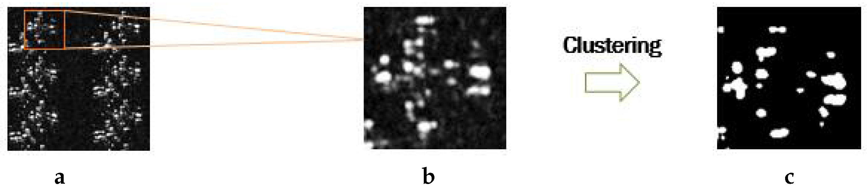
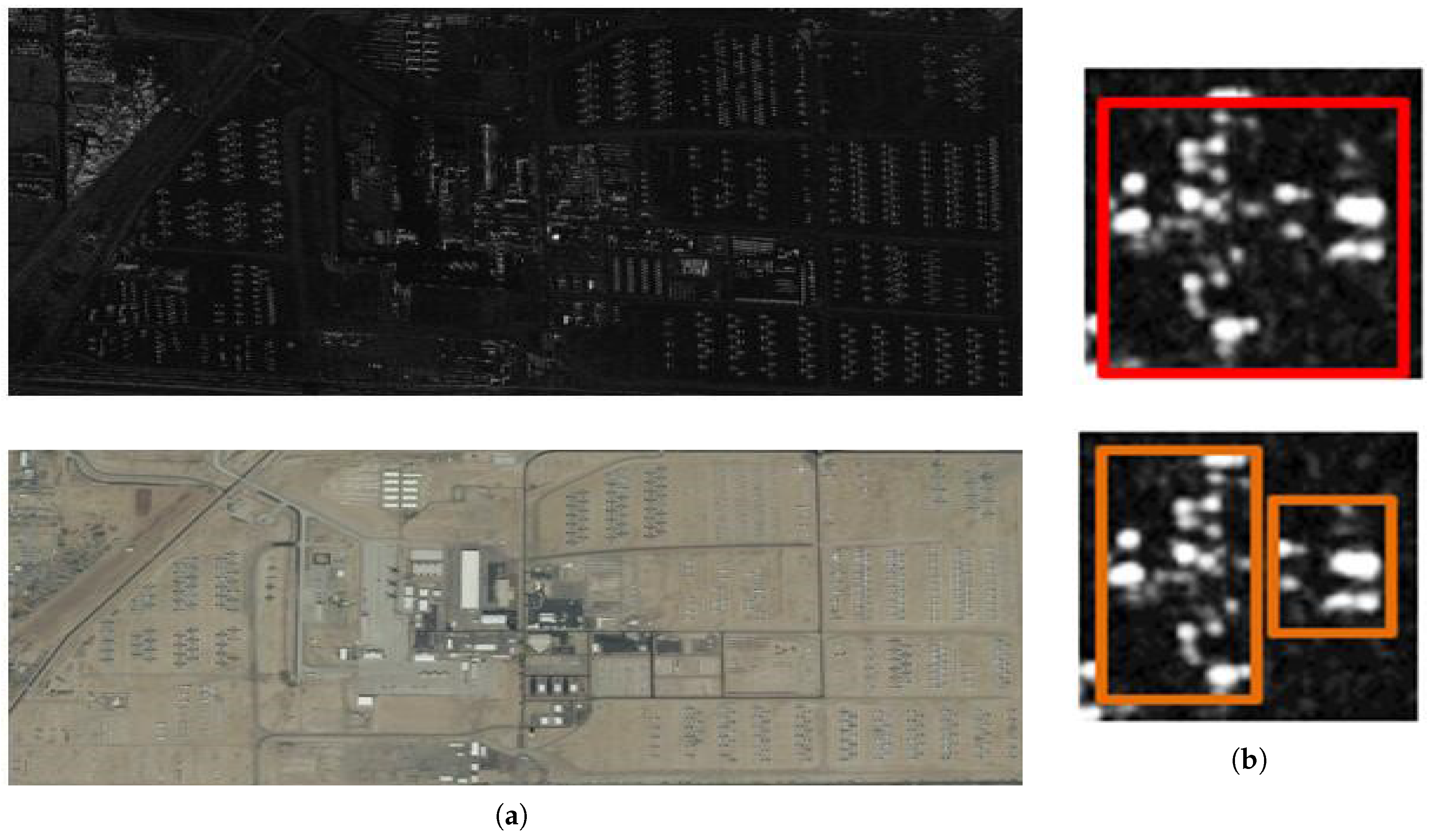
However, the existing target detection methods for SAR imagery still have some problems. Owing to the scattering mechanism in high-resolution SAR imagery, the airplane target in the image is presented as bright or dark scattering points [25], called sparsity (shown in Figure 1). Therefore, in some traditional detection algorithms, the object is divided into many small patches, making it difficult to be fully detected. Actually, each kind of object usually has some general architecture, composed of several similar components. Besides, each part is not independent, but has some unique spatial relationships. Hence, utilising the component features and the structural information is beneficial to achieve complete target detection.
To cope with the sparsity for airplane detection in SAR imagery, a multi-scale detector based on the deformable part model [26] is designed in this paper, which is comprised of a root filter and several corresponding part filters. With structure relationships taken into account, the root filter locates the whole aircraft in a rough scale and the part filters reconstruct the components at a higher resolution. The root model and part models are trained through a potential support vector machine (SVM) [27,28]. After the initialization, labeling samples are used for updating training to enhance the robustness of the overall model.
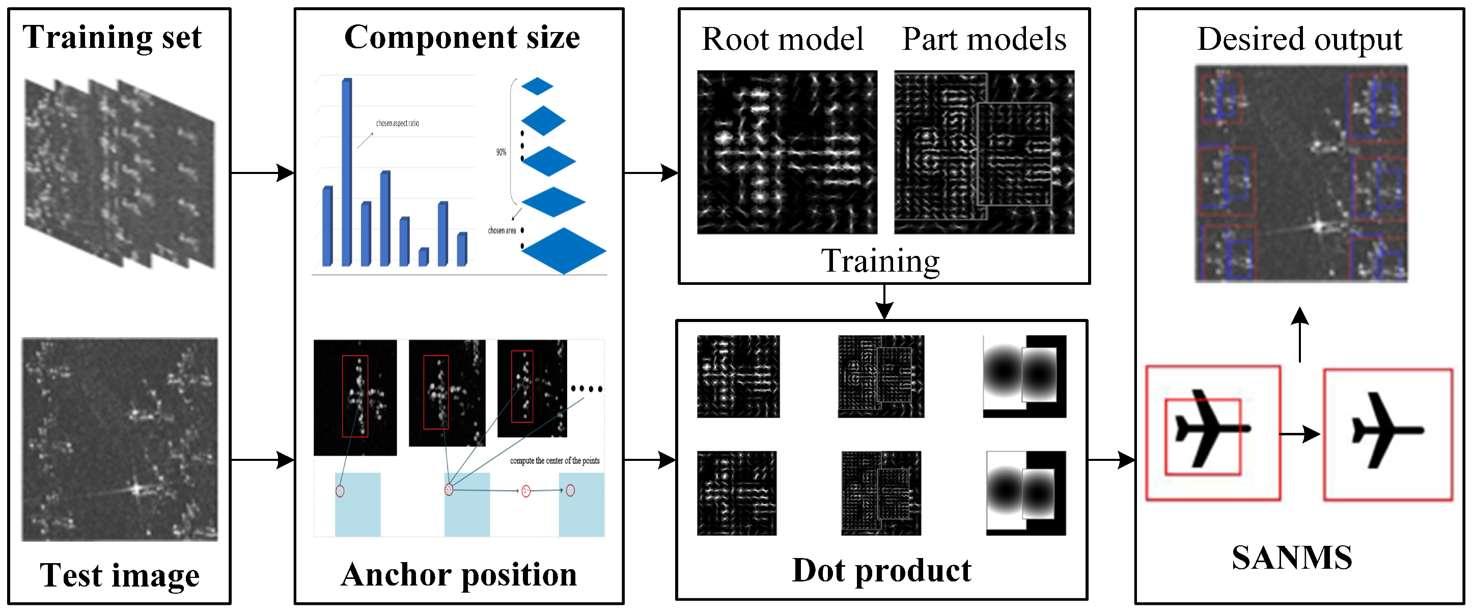
In this paper, the framework of the proposed Adaptive Component Selection-Based Discriminative Model (ACSDM) is shown in Figure 2. First, the training samples were divided into positive and negative categories, in which the target was labeled with a rectangular box. The coordinates of the top-left and bottom-right corners were recorded in an xml file. Then, statistical methods were adopted to determine the size and the anchor point for each component, respectively. It is worth noting that when training the model with SVM through gradient descent method [28], the penalty factor was added to the scoring formula to compensate information loss in preprocessing. In the detection stage, the dot product of the prediction operator and the test image was calculated. The position with high response was considered as a candidate result; meanwhile, the overall target was marked with a red box and the blue boxes marked the corresponding parts. Finally, a Small Area-Based Non-Maximum Suppression (SANMS) method was utilised to filter out the repeated bounding boxes.
2. Discriminative Model for Object Detection in SAR Imagery
Targeting the sparsity in SAR imagery, a discriminative scheme inspired by a multi-scale component hybrid model [26] is utilized to advance the detection performance. The original image is zoomed into different scales to obtain features in different layers, thus achieving a multi-scale feature pyramid; then, the model consisting of a root filter and several part filters with anchor information is built; finally, the part and component models are trained to generate a hybrid model, so as to realize the multi-scale deformable component mixture model. Taking advantage of component features and structure information, this multi-scale, deformable, and hybrid model can largely deal with the sparsity for detecting objects in high-resolution SAR imagery.
2.1. Root Filter and Part Filters
The multi-scale component model consists of a root filter that covers the entire target and corresponding part filters which reconstruct the target components in detail [6,29,30]. The root filter describes the target at a coarse resolution, and the part filters detect each component at twice the resolution of the root model, thus taking the spatial relationship among each component and the target into consideration. Before building the model, the histogram of oriented gradient (HOG) [31] feature pyramid must be constructed. After the original image is turned into a gray-scale map, it is divided into multiple 8 × 8 units. With the local histogram of the pixels in each unit counted, the 32-dimension HOG feature is obtained through linear interpolation and normalization. Finally, the feature pyramid is formed with images of different resolution, processed as above.
For a sliding window () in the HOG space, a corresponding weight vector is put in the root filter. Assuming that H stands for the HOG feature pyramid, p = (x,y,l) represents the detection box in the pyramid level. indicates the eigenvector of the sliding window with p as its top-left corner. The score of the root model is equal to the inner product of the weight vector and the feature, simplified as .
Supposing that a target is divided into n components, represented by , in which means the part model. denotes the position offset of the component box in the root window, is the box size, and , represent the deformation cost together. In view of the loss caused by the position offset, the score of the component model is expressed as follows:
where is the coordinate of the root filter in the pyramid and 2 stands for that of the part filter. indicates the undeformed part filter’s position (i.e., anchor point). means the offset of the component’s actual position to its anchor point, measuring the deformation degree. In that case, the deformable model is realized by subtracting the corresponding deformation cost when calculating the score.
Representing the filter vectors and deformation parameters with , and stands for the detection boxes’ feature and location:
Therefore, the scoring formula in the spatial position z is modified as .
2.2. Model Training
In the model training phase, the first step is to initialize the size and weight of the root filter. In general, the average size of the labeled rectangle in positive samples is taken as the root filter size. The negative samples are cropped arbitrarily from the background which is irrelevant to the target. After extracting the HOG feature for each sample, the root filter is initialized by standard SVM with zero value.
For the initialization of the component filters, the root filter’s energy, that is the L2 norm of the weights, is calculated firstly. Then, the total energy of the 6 × 6 rectangle region with a certain point as the upper-left corner is counted. The point related to the 6 × 6 rectangle with the maximum energy is regarded as the anchor position, and the weight in the region is the initialized weight for the component model. Following the principle of non-overlapping, the anchor of other components are initialized in the same way.
After initialization, the components are not in their actual positions, so the latent SVM method is employed for updating training, whose purpose is to obtain weights in model . Besides, to improve the model robustness, it is necessary to add some difficult samples to the training set. Supposing that the sample set is , means the sample class and corresponds to positive and negative samples, respectively. In each sample, the positions of the components are regarded as hidden variables. The objective function of the model parameters is expressed as:
where max is the standard hinge loss function, and C represents the normalized weight. Since the target is not contained in negative samples, the coordinates of the component filters need not be determined, and thus the objective function has an optimal solution. That means that while , max becomes a linear convex function. When training with positive samples, the current coordinates of the filter boxes are taken as fixed values, and thus the objective function is converted into a convex function. The value of is obtained by continuous iteration until the function converges.
2.3. Object Detection
When the deformable part model is used for target detection, the sliding window goes through each scale of the feature pyramid in order to get a score of each possible location. In the detection window, the score of the root filter is calculated first, then the maximum score of each component filter in the corresponding resolution is obtained. Therefore, in the pyramid, the final score of the current detection window is equal to the sum of the root filter score, the component filter score, and the deformation cost. The overall scoring formula is as follows:
is the detection score of the root filter, denotes the response of the part filter, and b is the offset coefficient. Before calculating the part contribution, the optimal positions of different part filters must be acquired. When the whole discriminant score is higher than the threshold, it indicates that the target boundary has been detected and the component filters have detected each component, thus achieving the detection of the complete target. The detected bounding box from the newly trained model is usually offset to a certain extent; in order to obtain a more accurate bounding box, linear least-squares regression [32] is utilized for optimization. The coordinates of the root bounding box and n part bounding boxes (2n + 3 dimension) are utilised to predict a more accurate bounding box for the target. Finally, the Non-Maximum Suppression [33] method is applied to filter out the duplicate results.
3. Adaptive Component Selection-Based Discriminative Model
In the multi-scale component-based discriminative model, the structure information can effectively cope with the sparsity in SAR imagery. However, the size of different components is a fixed value: 6 × 6.
Figure 3a,b present the results for pedestrian and airplane detection with Felzenszwalb’s model, in which different resolutions are selected for different object categories, but not for the components in the target. As shown in Figure 3a, a detected person has five components, and each one is labelled with a 6 × 6 bounding box (blue) in the final detection. From the aircraft detection shown in Figure 3b, it is clear that the two components (the airplane head and the tail) are also detected with 6 × 6 bounding boxes (blue). Besides, when initialising the component model, the weight’s norm in different 6 × 6 regions of the root model are calculated, and the one with the maximum norm is taken as the component location. This means that the top-left corner of the region is regarded as the anchor point and the component is simply placed in the 6 × 6 region with high energy. In response to the problems above, the desired output of the ACSDM approach is shown in Figure 3c; the airplane head and tail are detected with appropriate size, matching the actual target more closely. Therefore, better strategies are needed to solve the following problems: (1) the size of the component is fixed, always be 6 × 6; (2) the anchor position of the component is determined by the region energy, not showing its real position.
3.1. Adaptive Selection of the Component
In response to the problems above, a different scheme is considered in the proposed ACSDM algorithm. The component size is no longer fixed, but obtained through the statistical samples. Meanwhile, the anchor point is no longer decided by the root model energy, but determined according to the component location. In this way, the components in the training samples also need to be labeled. The adaptive selection of the component consists of two procedures: the determination of the component size and the anchor position.
3.1.1. Determination of the Component Size
In order to detect accurate components, the fixed size is no longer suitable. Generally, the sizes of various components in a target are usually not the same. For different types of objects, the components’ sizes are more distinct. In this ACSDM algorithm, a method based on the components’ scale information in the statistical samples is employed to determine the appropriate size.
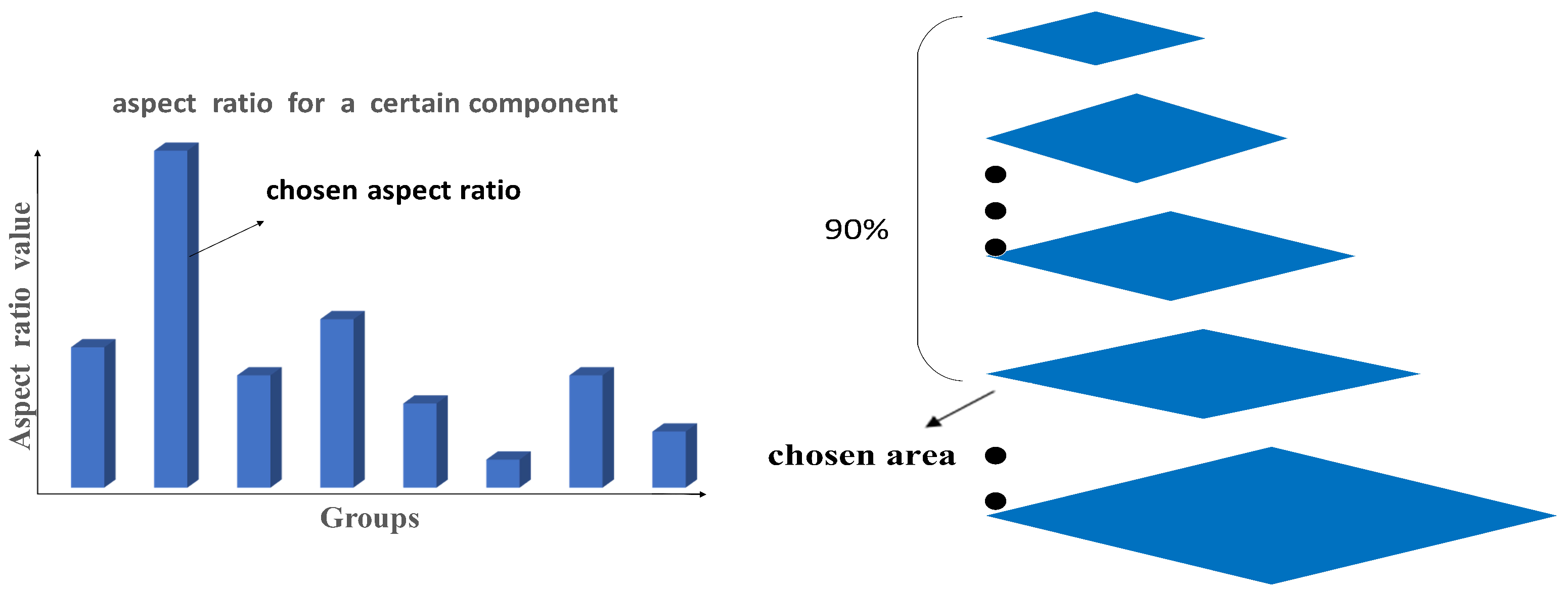
As shown in Figure 4, for a certain component, the ratio (height to width) in positive samples is classified into several groups. The aspect ratio is generally in the range of 0.5–2.5, and a group is divided at every 0.25 step. The aspect ratio value of y axis is the average ratio of the corresponding group. The ratio value of the highest histogram is determined as the that of the component. Meanwhile, through the coordinates information in the xml file, the bounding box area of each component is computed and reordered from small to large, and the area at the 90% position is decided as the standard value. In that case, the height H and width W are acquired through Equations (7) and (8). For different components, the same method is applied to calculate the corresponding H and W. The essence of selecting the aspect ratio through histogram is that one specific component in most samples has a similar aspect ratio. Simply computing the average value cannot deal with some special circumstances. If bad samples with quite different ratio appear in the training set, it will have a great impact on the average ratio. Indeed, the aspect ratio reflects its component class to a certain extent, and the statistical method can reduce the influence of bad samples. However, as the target has various depth in the image, the area of the same target can be different. In order to detect as many components as possible, the area of the components is set at the value of the 90% position.
3.1.2. Determination of the Anchor Position
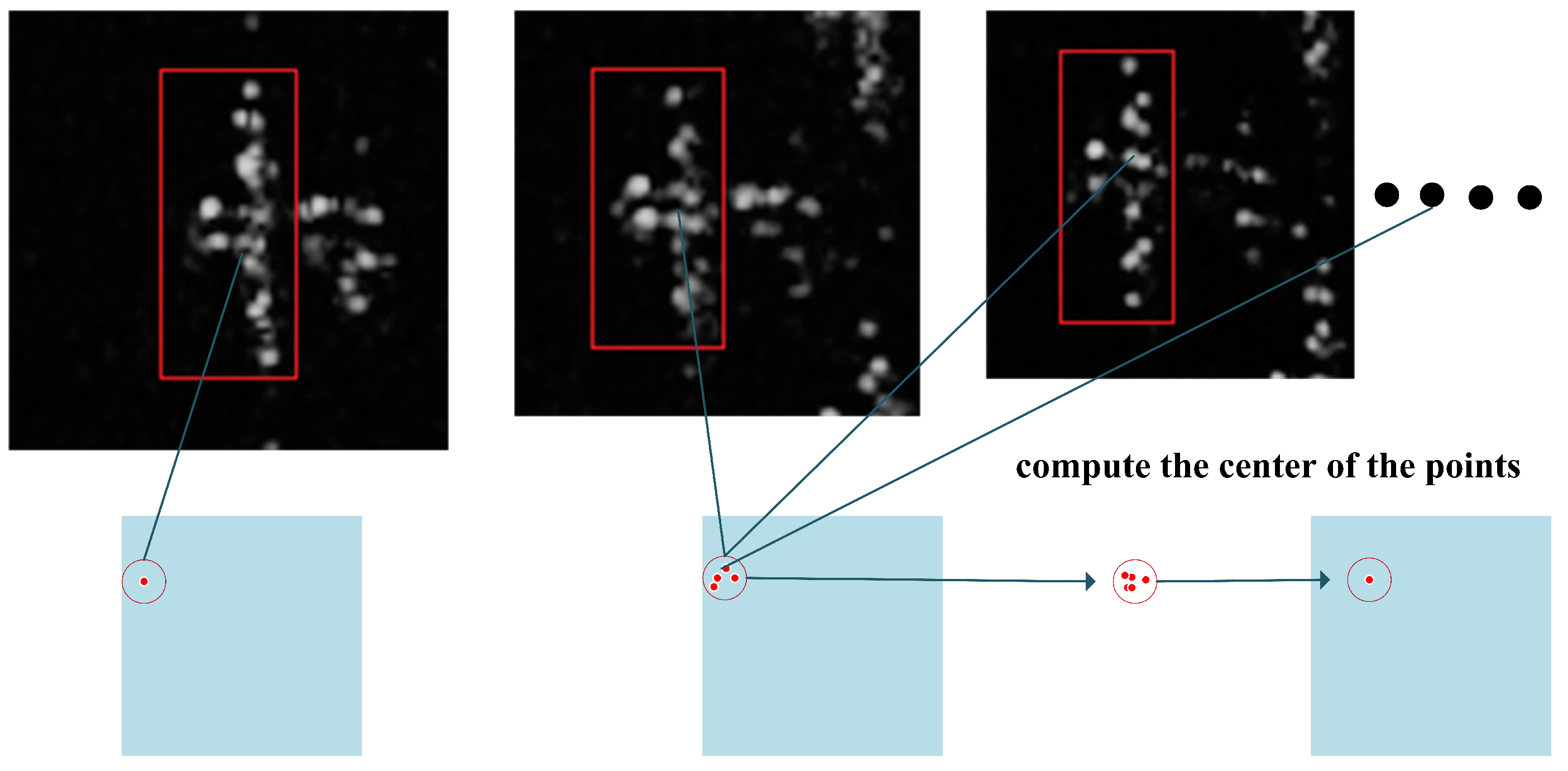
The detected results of the component are related to the size and the anchor point. In the ACSDM algorithm, the method to decide the anchor position is shown in Figure 5. For the head component in an aircraft, the relative coordinates of the component center to the red bounding box are calculated and normalized. With the central coordinates of the same component-class processed above, the anchor location is obtained by mean filtering [34]. For components in different types, the anchor point is acquired in the same way. In high-resolution SAR images, different attitude, incidence angle of the radar wave, or different terrain lead to various aircraft shapes, which means the component position is offset to different degrees. If all targets employ a fixed anchor point, the results are definitely unsatisfactory. Using mean filter to select the anchor point makes the located component more practical, but of course the accuracy will decrease.
With the scheme above, the initialization for the component model becomes different. First, the size and anchor point for each component are determined through statistical methods; then, the weight in the rectangle (H × W) with the anchor point as its upper-left corner is obtained as the initial value for the component model.
3.2. Training and Detection of the ACSDM Algorithm
In the training stage, in order to minimize information loss in preprocessing, a penalty factor is introduced into the scoring formula for compensation. In addition, in the object detection stage, the SANMS method is employed to remove the redundant bounding boxes, which also reduces the false alarm rate.
3.2.1. Introducing the Penalty Factor in the Training Process
In SAR imagery, large object number and different poses lead to various aspect ratios. When positive samples are preprocessed, excessive deformation will occur in building the feature pyramid, causing image information loss. In response to this problem, a proportional penalty factor is introduced into the score equation for training with SVM. With the image loss taken into account, the scoring formula is modified to be more reasonable, and is shown as follows:
where is the proportional penalty factor, dhw is the difference between the target’s aspect ratio and the root model, is a negative value. The larger the dhw is, the greater the inhibition on the score. Therefore, the information loss caused by sample-size unification is compensated.
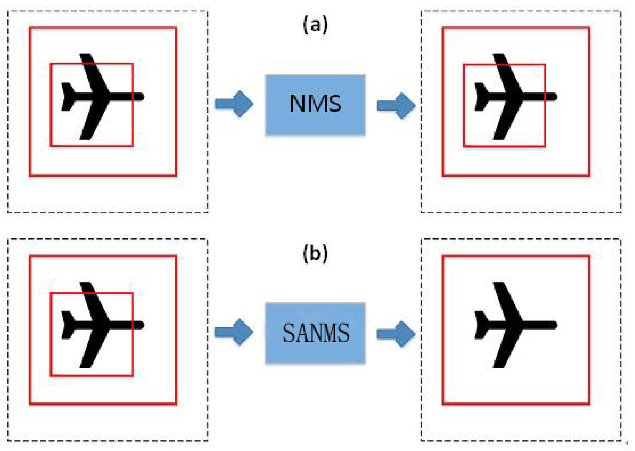
3.2.2. SANMS Method in the Detection
In SAR imagery, the aircraft target is usually small and highly-centralized, and thus duplicate detection results are more likely to occur. The Non-Maximum Suppression algorithm based on greedy strategy is widely utilized to eliminate duplicate detection. In its main idea, the detection results are sorted and the one with the highest score is selected. Then, other results overlapping with the chosen one by more than 50% are filtered out. However, this method misses the situation where a high-score bounding box overlaps with the lower-score one, as the overlap rate is calculated as follows:
Among them, is the higher-score bounding area while is the lower-score bounding box, and indicates the overlap area between them. As shown in Figure 6, if is completely contained in and the area of is less than half of , the duplicate results will not be filtered out.
To reduce the redundant bounding box, the calculation formula of the overlap rate is modified. As shown in Equation (11), the denominator is replaced by the smaller of the two bounding boxes. Accordingly, it is called the Small Area-Based Non-Maximum Suppression (SANMS) method.
In this way, even if the small detection box has a higher score, it can be filtered out. This method cannot only filter the detection frames of similar size, but also works for frames with quite different size.
4. Experiments
4.1. Experimental Data and Evaluation
The experimental data in this paper is derived from TerraSAR-X imagery with HH band, at Mount Davies Air Force Base, Arizona. The resolution of the high-resolution SAR imagery is 2 meters, and the image size is 11,296 × 6248. The original SAR imagery containing over 820 aircrafts and the corresponding optical image are shown in Figure 7. Besides, the whole imagery is cut into 120 sampling pictures with 110 for training and the rest for testing. Unlike the availability of optical images, it is quite difficult to obtain high-resolution SAR imagery containing many aeroplanes because of its high price and military restrictions. Although the experimental dataset looks a bit small, cross-validation is considered to avoid overtraining. To mark the target more accurately, the training set is labelled combining with September 2010 Google Earth optical image. To determine the size and anchor point for each component, the aircraft parts also need to be marked. In this paper, an aeroplane is divided into two components: the head and the tail. Therefore, each target is labeled with one global bounding box and two component bounding boxes, also shown in Figure 7.
To assess the performance of each algorithm accurately, a unified criterion is adopted for appraisal. This paper uses three indexes to evaluate the detection results: (1) the detection precision P; (2) the false alarm rate ; (3) the detection recall rate R. The detection precision stands for the proportion of correctly detected airplanes in all detected objects; the detection false alarm rate means the proportion of wrongly detected aircrafts in all detected objects; the recall rate represents the proportion of correctly detected targets in the total airplanes. The specific formulae for three kinds of accuracies are calculated as follows:
In Equation (12), means the number of all detected objects, and and represent the number of correctly detected aircrafts and objects that are falsely detected as aircrafts, respectively. Therefore, . indicates the number of total aircrafts, including the correctly detected aircrafts and the missing number; in the following experiments, . These indexes are counted in each image individually, then the overall measurement indexes are added up and computed.
4.2. Detection Method Based on CFAR
4.2.1. Experiment Settings
As a classical detection approach, experiments about the method based on CFAR were conducted for comparison. Specifically, the CFAR-based method and clustering were combined to detect aircrafts in SAR imagery. The statistical feature used was the Weibull model, and a CA-CFAR statistical model was utilized to detect the clustering frame of the highlighted points. To demonstrate the sparsity of the scattering targets in SAR images, the preliminary detection results of the CFAR method are presented, and the final detection results after clustering are also shown in Table 1. The false alarm probability is set to be .
4.2.2. Experimental Results
As shown in Table 1, aeroplanes in ten different sub-regions were selected for detection. In the preliminary CFAR results, there is no box, but only a clustering of scattering points. It can be seen that these strong highlighted scattering points that make up the planes are divided into many small patches, reflecting the sparsity in the SAR imagery. In addition, the scattering points are presented as various arrangements , indicating the diversity. It is the particularity above that makes the final detection results unsatisfactory. In the final detection results, some scattering points and even the airplane tails are detected as a target, showing that the CFAR-based method cannot identify the components clearly. 3.5pt
The statistical data is presented in Table 2. In the CFAR-based algorithm, it is calculated that the detection precision P = 73.2%, the false alarm rate = 26.8%, and the recall rate R = 93.2%. From these results, it is clear that the method based on CFAR for target detection in high-resolution SAR imagery is not reliable enough. Despite the high recall rate, the false alarm rate is rather large, with 40 wrongly detected objects in the total 117 aeroplanes, and the detection precision is unsatisfactory. Besides, it is obvious that some airplanes are detected as one target. Therefore, the CFAR-based detection algorithm is not effective for airplane detection in the SAR imagery.
4.3. The Discriminative Model Based on the Multi-Component Scheme
Since the proposed ACSDM algorithm is inspired by the discriminative model, several experiments were conducted to illustrate the difference. The penalty factor, adaptive component selection, and SANMS were separately added to the discriminative model to generate three comparative schemes. Considering that listing the results of ten testing images occupies a large area, for the three different methods above, another two experimental images are listed for analysis.
4.3.1. Experiment Settings
In this paper, the whole SAR imagery was divided into 120 figures, where 10 of them were used for testing images and 110 pictures served as training images. As a supervised learning method, two components (the head and the tail) in the training set of SANMS need labeling. Each positive sample was labeled with a global bounding box and two component bounding boxes (as shown in Figure 7), while some highlighted areas of non-target region were defined as “other” type to extract negative samples for training.
4.3.2. Experimental Results
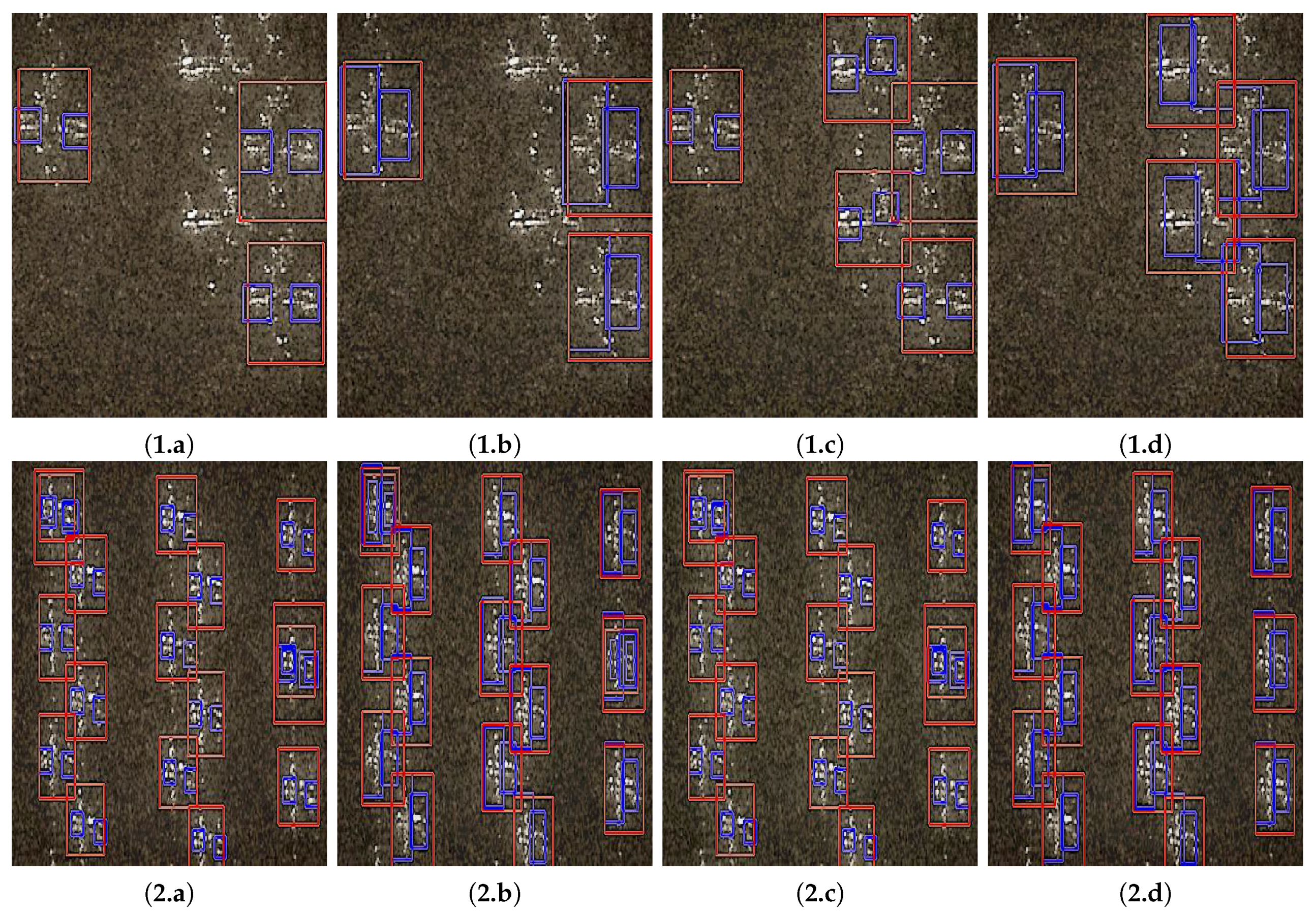
The comparative results are presented in Figure 8; it is clear that the three improved schemes do improve the detection performance. There are five aircrafts in testing region 1, but Figure 8(1.a) shows that the discriminative model could detect only three aircrafts, and the size of the two detected components in the image is a fixed value: 6 × 6, which does not match the size of the actual head or tail. Figure 8(1.b) shows the result of the discriminative model with adaptive component selected, in which the detected component size matches its actual size. In Figure 8(1.c), the discriminative model introduces the penalty factor into the score formula. With information loss in preprocessing compensated, the number of detected targets increased to five. Given that the redundant detection boxes do not appear, the results of the discriminative model with SANMS added are not presented. The detection results of the ACSDM method are displayed in Figure 8(1.d). Comparing with the detection in Figure 8(1.a), there are improvements both in the detection precision and the matching degree of component size.
In testing region 2, enhancement brought by adaptive component size selection is still very obvious—contrast in Figure 8(2.a) and Figure 8(2.b) is very clear. However, the penalty factor does not show any effect; Figure 8(2.a) and Figure 8(2.c) are almost the same—all 15 aircrafts were detected by the discriminative model. However, in the detection of Figure 8(2.a), two planes were detected with duplicate bounding boxes (the first in the first column and another in the third column). In response to this problem, the SANMS method was utilized to filter out the redundant boxes. Through the ACSDM algorithm, each aircraft was detected with a global bounding box (red) and two component bounding boxes (blue), as shown in Figure 8(2.d), which proves the validity of the SANMS method.
It is worth noting that the statistical indexes of the above methods are calculated and displayed in the conclusion, although the data are not listed. With adaptive component selection, the detected component size fits the actual target more closely. Meanwhile, the introduced penalty factor improves the detection precision, and the SANMS method reduces the false alarm rate effectively.
4.4. The ACSDM Method
4.4.1. Experiment Settings
In Section 4.3, partial experimental results about the ACSDM method were demonstrated. In this section, detailed results and analysis are presented for comparison. The testing data adopted was the same as that in the previous section, with 10 images for testing and the rest for training. There were still two components in the aeroplane: the head and the tail. It should be noted that the number of components was determined by experience and actual situation. Since the aircraft in the SAR imagery are rather small, it would be difficult to separate the target into many components. Otherwise, the size for each component would be too small for feature extraction. Taking these factors into consideration, an aircraft consisting of two components is appropriate. Additionally, the way of labelling both positive and negative samples was the same as that in Section 4.3, and the maximum number of iterations was set to 10,000. When the model training finished, the obtained threshold was used for testing, although it was a rough value at that time. Then, the threshold was adjusted through the testing of another few images. Finally, the optimal threshold was selected for the following detection. In that case, the threshold had less influence on the detection results, assuring that the performance of the different algorithms can be fairly compared.
4.4.2. Experimental Results
The detection results of the ACSDM method are shown in Table 3, and the statistical data are shown in Table 4. It was calculated that the detection precision P = 96.4%; the false alarm rate = 3.6%, and the recall rate R = 91.5%.
As can be seen from Table 3, the targets were accurately detected and the components were located in their actual positions. Meanwhile, the case that an aircraft is detected as several targets did not occur, indicating the effectiveness of component information in coping with the sparsity in SAR imagery. However, there were still airplanes which were not detected, and some objects were wrongly detected as airplanes. Compared with the performance of the CFAR-based method, the missing detection number in that of the ACSDM method was quite similar, but the wrongly detected number in the proposed method was largely reduced.
4.5. Analysis
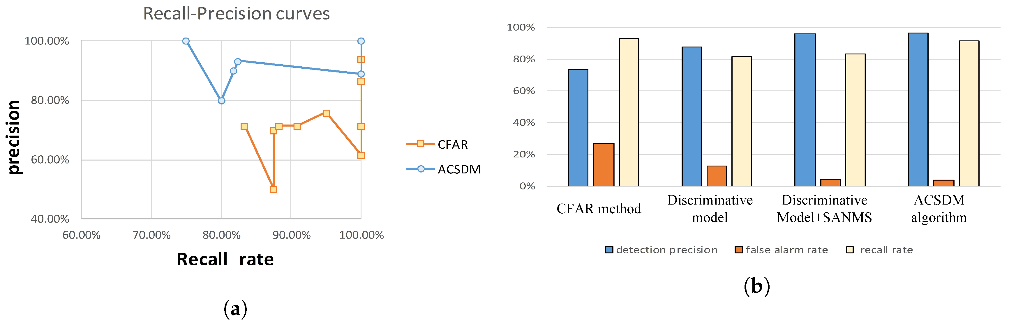
The measurement indexes of the detection results in different methods are shown in Figure 9. In the ten testing images, the recall-precision curves of the CFAR-based method and the presented ACSDM approach are displayed (shown in Figure 9a). Indeed, there are ten points in each curve, but some points have the same precision and recall rate. From the presented curves, it is clear that the average precision is higher in the ACSDM model, in which the recall rate is a bit lower.
In the testing results of the CFAR-based method, a large number of false alarms occurred due to the sparsity in the SAR imagery. The strong scattering points of the airplane were segmented to small patches, increasing the error detection rate. The case where several aeroplanes were detected as one target also appeared, resulting in missing detection. The reason is that the airplanes in the image are highly concentrated, and the scattering points belonging to adjacent aircrafts are difficult to identify. There are 40 error-checks in 10 testing images, which indicates that the CFAR-based method is not effective in dealing with aircraft detection in SAR imagery. As for the discriminative model, its detection precision decreased to 87.6%, and the false alarm rate dropped to 12.4%. Even though the results were better, there were many duplicate detection boxes because Non-Maximum Suppression in this approach was insufficient. In response to this, a discriminant model combined with the SANMS method was employed for experiments, achieving performance with a detection rate of 95.9% and false alarm rate of 4.1%, which proves the validity of the SANMS method for filtering duplicate boxes.
In the detection with the presented ACSDM algorithm, the false alarm rate was 3.6% and the detection rate was 96.4%. There were few wrong detections and missing detections, since component structure provides useful information for airplane detection. Though the strong scattering points of a target were separated into several parts, they could still be effectively united together. Meanwhile, these scattering points belonging to adjacent airplanes could also be distinguished, reducing the false alarms. Although the recall rate was slightly lower in the ACSDM algorithm, its detection rate was much higher than that of the CFAR-based method. From Figure 8 and Table 4, it is clear that in the presented algorithm, the multiple bounding boxes were largely reduced owing to the SANMS method, and thus the false alarm rate decreased greatly. In addition, the aircraft’s head and tail were correctly detected and the component size was more appropriate, illustrating the effectiveness of adaptive component selection. Further, the detected components are of practical significance, making the overall target detection more accurate.
4.6. Discussion
To further improve the accuracy and apply the proposed method in practical situations, the following aspects are considered.
(1) Selection of HOG feature
This ACSDM algorithm introduces the DPM model [26] with good performance on optical images, and DPM is based on the HOG feature to extract the basic segments. We understand that optical image is an additive model while SAR imagery is a multiplicative model. Therefore, the gradient algorithm in HOG is often replaced by a ratio algorithm for SAR images in order to get transform segments. We tried an algorithm where segments are extracted through the histogram of ratio method, but we have not yet achieved a better result.
The HOG feature is still used in the bottom of the ACSDM algorithm. Although the aircrafts are presented as scattering points in SAR imagery, owing to the special imaging mechanism. The target structure is still obvious and the extracted segments are combined for object detection, not for contour extraction. The essence of the HOG feature is that it can effectively describe the gradient, which also applies for objects with clear structure in SAR imagery.
(2) Rotational invariance
In our paper, all the airplanes in the training set have similar positions, the airplane head faces to the left, followed by the tail. Therefore, the trained model is suitable for detecting aircrafts with this orientation. While the original testing images are rotated by 90 and −90 degrees, the airplane components are not detected by the model anymore. However, a good thing is that this model can be trained. when we add all the 90 and −90 degrees images to the training set, a different model is generated. In addition, the corresponding detection results are shown in Figure 10.
From the detection results, it is clear that the detected objects(with bounding boxes) are the airplane targets, thus . According to the calculating formula, the precision P = 100%. However, 30 airplanes are not detected, the recall precision R = 87/117 = 74.4%. Especially, in region 3-8, a lot of airplanes are missing. Therefore, the model trained with airplanes in similar positions cannot detect rotated airplanes effectively, but the newly trained one can cope with the rotation variation to some degrees.
5. Conclusions
This paper presents an ACSDM algorithm for airplane detection in high spatial resolution SAR imagery. To cope with the sparsity, a multi-scale detector including a root filter and several component filters was built for aircraft detection. In order to detect the components more accurately, two statistical methods were employed to determine the appropriate size and anchor point for each component. Besides, in the model initialization stage, a penalty factor was introduced into the scoring formula to minimize the image information loss in preprocessing. For the candidate results, the SANMS method was utilized to filter out the redundant bounding frames in the same target. In this paper, the ACSDM algorithm is tested on a TerraSAR-X SAR data set with the CFAR-based method for aircraft detection. The results demonstrate the effectiveness of the proposed method by achieving the highest detection rate, which proves the validity of spatial structure. Although the recall rate of ACSDM approach was a little lower than that of the CFAR-based method, the higher false alarm rate in the latter method is also not negligible. Besides, in the experiments evaluating the ACSDM algorithm and a series of discriminative models, the presented method also provided the best results with the highest precision and the lowest false alarm rate, owing to the introduced penalty factor and the SANMS method. Moreover, the components such as the airplane head and the tail were clearly detected, matching their actual sizes in the image, showing the effectiveness of adaptive component selection. Future work will be focused on utilising more efficient features to replace the original HOG feature in the improved algorithm in order to enhance the describing ability for the target.
Acknowledgments
This work was partially supported by the National Natural Science Foundation of China (No.41371342,No.61331016), and by the National Key Research and Development Program of China (No.2016YFC0803003-01).
Author Contributions
Chu He and Mingxia Tu conceived and designed the experiments; Dehui Xiong performed the experiments and analyzed the results; Chu He and Mingxia Tu wrote the paper; Feng Tu and Mingsheng Liao revised the paper.
Conflicts of Interest
The authors declare no conflict of interest.
Abbreviations
The following abbreviations are used in this manuscript:
| ACSDM | Adaptive Component Selection-Based Discriminative Model |
| SAR | Synthetic Aperture Radar |
| SANMS | Small Area-Based Non-Maximum Suppression |
| CFAR | Constant False Alarm Rate |
| CA-CFAR | Cell Average CFAR |
| OS-CFAR | Ordered Statistics CFAR |
| GO-CFAR | Greatest Opt-CFAR |
| SO-CFAR | Smallest Opt-CFAR |
| MRF | Markov Random Fields |
| R-CNNs | Regions with Convolutional Neural Networks |
| YOLO | You Only Look Once |
| SVM | Support Vector Machine |
| HOG | Histogram of Oriented Gradient |
References
- Van, Z.; Kim, Y. Synthetic Aperture Radar Polarimetry. In Proceedings of the IEEE Seventh International Conference on Image and Graphics, Qingdao, China, 26–28 July 2013; pp. 343–347. [Google Scholar]
- Borowiec, K. Application for Displaying Synthetic Aperture Radar Imagery in Real-time Implementation and Results. Int. J. Electron. Telecommun. 2016, 61, 4–8. [Google Scholar]
- Argenti, F.; Lapini, A.; Bianchi, T. A Tutorial on Speckle Reduction in Synthetic ApertureRadar Images. IEEE Geosci. Remote Sens. Mag. 2013, 1, 6–35. [Google Scholar] [CrossRef]
- Jackson, J.A.; Rigling, B.D.; Moses, R.L. Canonical scattering feature models for 3D and bistatic SAR. IEE Trans. Aerosp. Electron. Syst. 2010, 46, 525–541. [Google Scholar] [CrossRef]
- Badri, N.S.; Susmita, G.; Simon, C.K.S.; Ashish, G. Statistical Feature Bag based Background Subtraction for Local Change Detection. IEEE Inf. Sci. 2016, 366, 31–47. [Google Scholar]
- Cheng, G.; Han, J. A survey on object detection in optical remote sensing images. ISPRS J. Photogramm. Remote Sens. 2016, 117, 11–28. [Google Scholar] [CrossRef]
- Irving, W.W.; Ettinger, G.J. Classification of targets in synthetic aperture radar imagery via quantized grayscale matching. In Proceedings of the SPIE—The International Society for Optical Engineering, Orlando, FL, USA, 13 August 1999; pp. 21–37. [Google Scholar]
- Keller, J.B. Geometrical Theory of Diffraction. J. Opt. Soc. Am. 1962, 52, 116–130. [Google Scholar] [CrossRef] [PubMed]
- Gerry, M.J.; Potter, L.C.; Gupta, I.J.; Van Der Merwe, A. A parametric model for synthetic aperture radar measurements. IEEE Trans. Antennas Propag. 1999, 47, 1179–1188. [Google Scholar] [CrossRef]
- Weinberg, G.V. Geometric mean switching constant false alarm rate detector. Dig. Signal Process. 2017, 69, 1–10. [Google Scholar] [CrossRef]
- Finn, H.M.; Johnson, R.S. Adaptive detection mode with threshold control as a function of spatially sampled clutter-level estimates. RCA Rev. 1968, 29, 414–464. [Google Scholar]
- Kuttikkad, S.; Chellappa, R. Non-Gaussian CFAR techniques for target detection in high resolution SAR images. In Proceedings of the IEEE International Conference, Image Processing, Austin, TX, USA, 13–16 November 1994; pp. 910–914. [Google Scholar]
- Hansen, V.G. Constant false alarm rate processing in search radars. Radar-Present Future 1973, 105, 325–332. [Google Scholar]
- Trunk, G.V. Range resolution of targets using automatic detectors. IEE Trans. Aerosp. Electron. Syst. 1978, 5, 750–755. [Google Scholar] [CrossRef]
- Kapur, J.N.; Sahoo, P.K.; Wong, A.K.C. A new method for gray-level picture thresholdng using the entropy of the histogram. Comput. Vis. Gr. Image Process. 1985, 29, 273–285. [Google Scholar] [CrossRef]
- Weisenseel, R.A.; Karl, W.C.; Castanon, D.A.; Brower, R.C. MRF-based Algorithms for Segmentation of SAR Images. ICIP Chic. 1998, 3, 770–774. [Google Scholar]
- Frery, A.C.; Yanasse, C.F.; Sant, S.J. Alternative distributions for the multiplicative model in SAR images. Geosci. Remote Sens. Symp. 1995, 1, 169–171. [Google Scholar]
- Goodman, J.W. Some fundamental properties of speckle. J. Opt. Soc. Am. 1976, 66, 145–150. [Google Scholar] [CrossRef]
- Stacy, E.W. A generalization of the gamma distribution. Ann. Math. Stat. 1962, 33, 1187–1192. [Google Scholar] [CrossRef]
- Umesh, C.P.; Pranab, K.D.; Alok, B. Feature Detection of an Object by Image Fusion. Int. J. Comput. Appl. 2010, 1, 50–57. [Google Scholar]
- Girshick, R.; Donahue, J.; Darrell, T.; Malik, J. Rich feature hierarchies for accurate object detection and semantic segmentation. In Proceedings of the IEEE Conference on Computer Vision and Pattern Recognition (CVPR), Toronto, ON, Canada, 23–28 June 2014. [Google Scholar]
- Girshick, R. Fast R-CNN. In Proceedings of the IEEE International Conference on Computer Vision (ICCV), Los Alamitos, CA, USA, 7–13 December 2015. [Google Scholar]
- Ren, S.; He, K.; Girshick, R.; Sun, J. Faster R-CNN: Towards Real-Time Object Detection with Region Proposal Networks. IEEE Trans. Pattern Anal. Mach. Intell. 2016, 39, 1137–1149. [Google Scholar] [CrossRef] [PubMed]
- Redmon, J.; Divvala, S.; Girshick, R.; Farhadi, A. You Only Look Once: Unified, Real-Time Object Detection. In Proceedings of the Computer Vision and Pattern Recognition (CVPR), Las Vegas, NV, USA, 27–30 June 2016. [Google Scholar]
- Tan, Y.; Li, Q.; Li, Y.; Tian, J. Aircraft Detection in High-Resolution SAR Images Based on a Gradient Textural Saliency Map. Sensors 2015, 15, 23071–23094. [Google Scholar] [CrossRef] [PubMed]
- Felzenszwalb, P.; Mcallester, D.; Ramanan, D. A discriminatively trained, multiscale, deformable part model. In Proceedings of the IEEE Computer Society Conference on Computer Vision and Pattern Recognition, Anchorage, AK, USA, 24–26 June 2008; pp. 1–8. [Google Scholar]
- Yan, Y. Multi-Classified Method of Support Vector Machine (SVM) Based on Entropy. IEEE Appl. Mech. Mater. 2013, 241–244, 1629–1632. [Google Scholar]
- Zhang, R.; Ma, J. An improved SVM method P-SVM for classification of remotely sensed data. Int. J. Remote Sens. 2008, 29, 6029–6036. [Google Scholar] [CrossRef]
- Han, J.; Zhang, D.; Cheng, G.; Guo, L.; Ren, J. Object detection in optical remote sensing images based on weakly supervised learning and high-level feature learning. IEEE Trans. Geosci. Remote Sens. 2015, 53, 3325–3337. [Google Scholar] [CrossRef]
- Han, J.; Zhou, P.; Zhang, D.; Cheng, G.; Guo, L.; Liu, Z.; Bu, S.; Wu, J. Efficient, simultaneous detection of multi-class geospatial targets based on visual saliency modeling and discriminative learning of sparse coding. ISPRS J. Photogramm. Remote Sens. 2014, 89, 37–48. [Google Scholar] [CrossRef]
- Navneet, D.; Bill, T. Histograms of Oriented Gradients for Human Detection. In Proceedings of the 2005 IEEE Computer Society Conference on Computer Vision and Pattern Recognition (CVPR’05), San Diego, CA, USA, 20–25 June 2005; pp. 886–893. [Google Scholar]
- Kenney, C.S.; Laub, A.J.; Reese, M.S. Statistical Condition Estimation for Linear Least Squares. Soc. Ind. Appl. Math. 2006, 19, 906–923. [Google Scholar] [CrossRef]
- Neubeck, A.; Van, G.L. Efficient Non-Maximum Suppression. In Proceedings of the 18th International Conference on Pattern Recognition (ICPR’06), Hong Kong, China, 20–24 August 2006; pp. 850–855. [Google Scholar]
- Wei, P.; Li, J.; Lu, D.; Chen, G. A Fast reliable switching median filter for highly corrupted images by impulse noise. IEEE Trans. Signal Process. 2007. [Google Scholar] [CrossRef]
Figure 1.
Sparsity in high-resolution SAR imagery. (a) Many aircraft targets; (b) One airplane extracted from Figure 1a; (c) The airplane is presented as scattering points after clustering.
Figure 1.
Sparsity in high-resolution SAR imagery. (a) Many aircraft targets; (b) One airplane extracted from Figure 1a; (c) The airplane is presented as scattering points after clustering.

Figure 2.
The overall framework of the proposed model. SANMS: Small Area-Based Non-Maximum Suppression method.
Figure 2.
The overall framework of the proposed model. SANMS: Small Area-Based Non-Maximum Suppression method.

Figure 3.
Different detection results. (a) Pedestrian detection in the discriminative model; (b) Airplane detection in the discriminative model; (c) Airplane detection in the Adaptive Component Selection-Based Discriminative Model (ACSDM) method.
Figure 3.
Different detection results. (a) Pedestrian detection in the discriminative model; (b) Airplane detection in the discriminative model; (c) Airplane detection in the Adaptive Component Selection-Based Discriminative Model (ACSDM) method.

Figure 4.
The determination of the aspect and the area.

Figure 5.
Determination of the anchor position.

Figure 6.
Different methods for filtering multiple detection boxes. (a) Non maximum suppression method; (b) Small area-based non maximum suppression method.
Figure 6.
Different methods for filtering multiple detection boxes. (a) Non maximum suppression method; (b) Small area-based non maximum suppression method.

Figure 7.
TerraSAR-X SAR data used in the experiments. (a) The original SAR imagery and the corresponding optical image; (b) The callout image: a global bounding box and two component bounding boxes.
Figure 7.
TerraSAR-X SAR data used in the experiments. (a) The original SAR imagery and the corresponding optical image; (b) The callout image: a global bounding box and two component bounding boxes.

Figure 8.
Detection results of the discriminative model and the ACSDM algorithm. (1.a) discriminative model; (1.b) discriminative model with adaptive component selection; (1.c) discriminative model with penalty factor introduced; (1.d) the ACSDM method; (2.a) discriminative model; (2.b) discriminative model with adaptive component selection; (2.c) discriminative model with penalty factor introduced; (2.d) the ACSDM method.

Figure 9.
Different measurement indexes. (a) Recall–precision curves; (b) Accuracies of different detection methods.
Figure 9.
Different measurement indexes. (a) Recall–precision curves; (b) Accuracies of different detection methods.

Figure 10.
Detection results of the newly trained model. (For a/b after each region, a represents number of the correctly detected airplanes; b is the number of total aircrafts in the region.)
Figure 10.
Detection results of the newly trained model. (For a/b after each region, a represents number of the correctly detected airplanes; b is the number of total aircrafts in the region.)


Table 1.
Experimental results of constant false alarm rate (CFAR)-based detection algorithm.
| Region | Labeled Image | Preliminary CFAR Detection Results | Final Detection Results |
|---|---|---|---|
| Region 1 |  |  |  |
| Region 2 |  |  |  |
| Region 3 |  |  |  |
| Region 4 |  |  |  |
| Region 5 |  |  |  |
| Region 6 |  |  |  |
| Region 7 |  |  |  |
| Region 8 |  |  |  |
| Region 9 |  |  |  |
| Region 10 |  |  |  |
Table 2.
The detection number of the CFAR algorithm.
| Correctly Detected Number Ncd | Missing Number | Wrongly Detected Number Nfd | |
|---|---|---|---|
| Region 1 | 10 | 2 | 4 |
| Region 2 | 19 | 1 | 6 |
| Region 3 | 8 | 0 | 5 |
| Region 4 | 5 | 0 | 2 |
| Region 5 | 10 | 1 | 4 |
| Region 6 | 15 | 2 | 6 |
| Region 7 | 7 | 1 | 3 |
| Region 8 | 7 | 1 | 7 |
| Region 9 | 15 | 0 | 1 |
| Region 10 | 13 | 0 | 2 |
| Total | 109 | 8 | 40 |
Table 3.
Experimental results of the ACSDM algorithm.
| Region | Labeled Image | ACSDM Detection Results |
| Region 1 |  |  |
| Region 2 |  |  |
| Region 3 |  |  |
| Region 4 |  |  |
| Region 5 |  |  |
| Region 6 |  |  |
| Region 7 |  |  |
| Region 8 |  |  |
| Region 9 |  |  |
| Region 10 |  |  |
Table 4.
The detection number of the ACSDM algorithm.
| Correctly Detected Number Ncd | Missing Number | Wrongly Detected Number Nfd | |
|---|---|---|---|
| Region 1 | 12 | 0 | 0 |
| Region 2 | 20 | 0 | 0 |
| Region 3 | 6 | 2 | 0 |
| Region 4 | 4 | 1 | 1 |
| Region 5 | 9 | 2 | 1 |
| Region 6 | 14 | 3 | 1 |
| Region 7 | 8 | 0 | 1 |
| Region 8 | 6 | 2 | 0 |
| Region 9 | 15 | 0 | 0 |
| Region 10 | 13 | 0 | 0 |
| Total | 107 | 10 | 4 |
© 2018 by the authors. Licensee MDPI, Basel, Switzerland. This article is an open access article distributed under the terms and conditions of the Creative Commons Attribution (CC BY) license (http://creativecommons.org/licenses/by/4.0/).
Share and Cite
MDPI and ACS Style
He, C.; Tu, M.; Xiong, D.; Tu, F.; Liao, M. Adaptive Component Selection-Based Discriminative Model for Object Detection in High-Resolution SAR Imagery. ISPRS Int. J. Geo-Inf. 2018, 7, 72. https://doi.org/10.3390/ijgi7020072
AMA Style
He C, Tu M, Xiong D, Tu F, Liao M. Adaptive Component Selection-Based Discriminative Model for Object Detection in High-Resolution SAR Imagery. ISPRS International Journal of Geo-Information. 2018; 7(2):72. https://doi.org/10.3390/ijgi7020072
Chicago/Turabian StyleHe, Chu, Mingxia Tu, Dehui Xiong, Feng Tu, and Mingsheng Liao. 2018. "Adaptive Component Selection-Based Discriminative Model for Object Detection in High-Resolution SAR Imagery" ISPRS International Journal of Geo-Information 7, no. 2: 72. https://doi.org/10.3390/ijgi7020072
Note that from the first issue of 2016, this journal uses article numbers instead of page numbers. See further details here.