Validation of HOAPS Rain Retrievals against OceanRAIN In-Situ Measurements over the Atlantic Ocean
by
 ,
,
Karl Bumke
1,*, 
Robin Pilch Kedzierski
1,
Marc Schröder
2,
Christian Klepp
3 and
Karsten Fennig
2 1
Marine Meteorology Department, GEOMAR Helmholtz Centre for Ocean Research Kiel, Wischhofstraße 1-3, 24148 Kiel, Germany
2
Deutscher Wetterdienst, Satellite Based Climate Monitoring, Frankfurter Straße 135, 63067 Offenbach, Germany
3
Faculty of Mathematics, Informatics and Natural Sciences, Department of Earth Sciences, CLiSAP/CEN, Universität Hamburg, Bundesstr. 55, 20146 Hamburg, Germany
*
Author to whom correspondence should be addressed.
Atmosphere 2019, 10(1), 15; https://doi.org/10.3390/atmos10010015
Submission received: 8 November 2018
/
Revised: 17 December 2018
/
Accepted: 28 December 2018
/
Published: 7 January 2019
(This article belongs to the Section Meteorology)
Abstract
:The satellite-derived HOAPS (Hamburg Ocean Atmosphere Parameters and Fluxes from Satellite Data) precipitation estimates have been validated against in-situ precipitation measurements from optical disdrometers, available from OceanRAIN (Ocean Rainfall And Ice-phase precipitation measurement Network) over the open-ocean by applying a statistical analysis for binary estimates. In addition to using directly collocated pairs of data, collocated data were merged within a certain temporal and spatial threshold into single events, according to the observation times. Although binary statistics do not show perfect agreement, simulations of areal estimates from the observations themselves indicate a reasonable performance of HOAPS to detect rain. However, there are deficits at low and mid-latitudes. Weaknesses also occur when analyzing the mean precipitation rates; HOAPS underperforms in the area of the intertropical convergence zone, where OceanRAIN observations show the highest mean precipitation rates. Histograms indicate that this is due to an underestimation of the frequency of moderate to high precipitation rates by HOAPS, which cannot be explained by areal averaging.
1. Introduction
Detailed knowledge of precipitation over the ocean is essential for understanding the global water cycle since it contributes to more than 75% of the global annual precipitation [1]. The sparsity of in-situ measurements of precipitation over the sea [2] results in remote sensing based data, such as the Hamburg Ocean Atmosphere Parameters and Fluxes from Satellite Data HOAPS [3], GPM (Global Precipitation Measurement [4]), and TRMM (Tropical Rainfall Measuring Mission [5]), or reanalysis data (e.g., ERA-Interim [6]), gaining growing attention,. While the HOAPS precipitation algorithm is based exclusively on SSM/I (Special Sensor Microwave Imager) and SSMIS (Special Sensor Microwave Imager/Sounder) passive microwave radiometers measurements, TRMM precipitation algorithms rely on measurements with an improved microwave radiometer, the TRMM Microwave Imager (TMI), and on measurements with a precipitation radar (PR) at 13.8 GHz. GPM precipitation is also derived from microwave radiometer measurements (the multichannel GPM microwave imager) and from measurements with a dual-frequency precipitation radar (DPR) at 35.5 GHz and 13.6 GHz. The resolution of both TRMM and GPM is 5 × 5 km2, which is considerably improved compared to HOAPS’ mean native pixel resolution of about 50 km. Precipitation products are publicly available [7,8,9], enabling validation studies on a global scale (e.g., Reference [10]). However, as References [6], [11], or [12] pointed out HOAPS, GPCP (Global Precipitation Climatology Project, e.g., Reference [13]) satellite retrievals and ERA-Interim reanalysis fields tend to show systematic deviations among themselves. Due to a lack of available precipitation in-situ data over sea [14], only a few validation studies of satellite-derived precipitation data against measurements over the ocean exist. For example, Reference [15] validated the TRMM Multisatellite Precipitation Analysis (TMPA, [5,16]) against buoys, showing an overestimation of TMPA over most of the buoy locations combined with an underestimation of high and light precipitation events. This underlines the need to perform more in-situ precipitation measurements over sea. Besides the efforts putting radars on research vessels (e.g., reference [17]), within the project OceanRAIN (Ocean Rainfall and Ice-phase precipitation measurement Network, [18,19]) a number of research vessels has successively been equipped with optical disdrometers [20], starting in 2010. Meanwhile, the amount of available data in OceanRAIN release 1.0 [21] allow for validating satellite-derived precipitation products, such as the HOAPS precipitation data. In this study, we will validate the HOAPS precipitation data [3] at their native pixel-level resolution of approximately 50 km in diameter against disdrometer measurements at 1 min resolution. The main problem is the comparison of areal averages with point or along track measurements (e.g., Reference [22]). To overcome this problem, we use binary statistics similar to the procedure of the German Weather Service validating their local model output against rain gauge measurements [23].
2. Data
2.1. HOAPS
The satellite-derived HOAPS climatology is, among other parameters, a compilation of precipitation and evaporation data to retrieve the net freshwater flux from one consistently derived global satellite data set over the ice-free oceans [24,25]. All variables are derived from SSM/I (Special Sensor Microwave Imager) and SSMIS (Special Sensor Microwave Imager/Sounder) passive microwave radiometers measurements, except for the SST (sea surface temperature), which is taken from AVHRR (Advanced very-high-resolution radiometer) measurements. Since the SSM/I records end in 2008, data used in this study are exclusively based on SSMIS. The HOAPS-precipitation retrieval is based on a neural network utilizing a training data set based on a one-dimensional variational retrieval that has been operated at ECMWF (European Centre for Medium-Range Weather Forecasts) between 2005 and 2009 [26,27]. Here we used the recently released HOAPS-4.0 precipitation product [3] at its native pixel-level resolution of approximately 50 km in diameter. It should be noted that the precipitation retrieval algorithm remains unchanged compared to the HOAPS-3.2 release. Since the sensitivity of the microwave imager hampers the detection of light rain below 0.3 mm·h−1, a lower threshold of 0.3 mm·h−1 was introduced, below which precipitation signals are set to zero [24]. Due to the strong influence of increasing emissivity of near land or ice-covered areas, HOAPS is also devoid of data within 50 km off any coastline or sea ice. HOAPS-4.0 comprises the period from 1987 until 2014. All HOAPS products have global coverage, i.e., within ±180° longitude and ±80° latitude. The products are also available as monthly averages and 6-hourly composites on a regular latitude/longitude grid with a spatial resolution of 0.5° × 0.5° degrees [7] (not used in our study).
2.2. OceanRAIN
OceanRAIN is a data set comprising in-situ shipboard precipitation, evaporation, freshwater flux, and meteorological data over the global oceans [18,19]. Precipitation data were gained by optical disdrometers of type ODM-470 [20] mounted on research vessels. Data are available for the period 2010 until 2017 as 1-min resolution along-track time series data. In the present study we use the OceanRAIN-W data set [19] of R/V Polarstern (2010–2014), R/V Meteor (2013–2014), and R/V Maria S. Merian (2012–2013) over the Atlantic Ocean; measurement periods are given in the brackets. Only measurements flagged as rain in the OceanRAIN-W data [21] at air temperatures above 4 °C [28] were used for validation.
The disdrometer data were cross-checked against ship rain gauge [29] measurements, which are part of the OceanRAIN-W data set (R/V Polarstern, R/V Meteor) or available from the Bundesamt für Seeschifffahrt und Hydrographie ([30], data from R/V Maria S. Merian is only available until 2013). Some discrepancies occur for measurements onboard the R/V Maria S. Merian from the 5 May 2013 onwards. Data from this period were excluded for the present study.
3. Methods
3.1. Collocation
According to an earlier study [31], the nearest neighbor approach was chosen for collocation with an allowed time difference of 45 min and a maximum distance of 55 km between the ship and the satellite‘s footprint. The maximum distance is derived from a study of Clemens and Bumke [32], who estimated the temporal scales of the precipitation measurements. Given that the ships move at about 15 km·h−1 average speed and based on 8-min measurements they calculated decorrelation lengths, defined as the distance at which the correlation decreases to the value of 1/e. They found decorrelation lengths of 46 to 68 km for stratiform and frontal precipitation and about 18 to 46 km for convective precipitation. Here we use a maximum distance of 30 km, which is approximately the mean value for convective precipitation. Adding the mean HOAPS pixel radius of 25 km we end up with a maximum distance of 55 km between the ships position and the satellite’s footprint. Allowed time differences were taken from a study of Klepp et al. [33], who investigated the influence of varying time windows in terms of dichotomous verification and for quantitative comparisons. For test purposes, allowed time differences and distances for collocation were reduced to 15 min and 25 km. This results in single collocated data pairs, consisting of one HOAPS pixel and one collocated OceanRAIN measurement. Further, all ship measurements within half an hour and the affiliated collocated HOAPS data were merged to single events lasting up to 2 h due to the allowed time differences used for collocation. Their spatial extension varies accordingly to the satellite’s footprints and the ships’ positions and speeds. Figure 1 depicts the positions of these events.
3.2. Statistical Analysis
The statistical analysis follows the recommendations given by the WMO (World Meteorological Organization) for binary or dichotomous estimates [34]. The method was applied to single collocated data pairs as well as on the events derived from the single collocated data pairs.
In total 12,791 events were available, comprising 2620 rain events, either measured by an optical disdrometer or retrieved from satellite estimates. These events were merged from 6,828,198 single pairs of collocated data. An average event includes about 30 measurements. Thus, each measurement is collocated approximately with 30 satellite pixels on average.
Each event was checked as a function of a lower threshold, applied to measured precipitation rates, to find whether the in-situ measurements and/or satellite data indicate precipitation. Measured precipitation rates below that threshold were set to zero. If one or more measured precipitation rates of an event exceeded that threshold, the event was flagged as “observed precipitation: yes”; if one of the satellite footprints of an event indicates precipitation, independent of its precipitation rate, the event was flagged as “HOAPS: yes”. Note that the minimum rain rate of HOAPS is 0.3 mm·h−1.
Following the recommendations stipulated by the WMO for binary or dichotomous estimates [34], 2 × 2 contingency tables are computed. They contain the hits (both HOAPS and measurements indicate precipitation), the correct negatives (both HOAPS and measurements indicate no precipitation), the misses (observation indicates precipitation in contrast to HOAPS), and the false alarms (HOAPS gives precipitation in contrast to measurements).
This allows us to derive the bias frequency, the probability of detection (POD), the false alarm ratio (FAR) and the EQuitable Threat score (EQT). The bias frequency answers the following question: how does the HOAPS frequency of “yes” events compare to the observed frequency of “yes” events? A bias frequency of 1 means that both data sets include the same number of precipitation events; a larger bias frequency indicates that there are more precipitation events in the HOAPS data. The POD gives the proportion of measured precipitation events, which can also be found in the HOAPS data, with 1 indicating perfect agreement and 0 no agreement, while the FAR gives the fraction of the observed no-events which were incorrectly forecasted as “yes”, with 0 indicating perfect agreement and 1 no agreement. The EQT measures the fraction of observed and/or forecasted events that were correctly predicted, adjusted for hits associated with random chance, no skill is indicated by −1/3; a perfect score equals 1.
3.3. Simulated Precipitation Fields
Comparing point/along-track observations with areal HOAPS estimates and the lower threshold of the HOAPS data are expected to hamper the statistics. Thus, to gain an idea of reasonable numbers for the statistical analysis of collocated along-track measurements with areal/temporal averaged estimates, simulations of in-situ observation data sets and corresponding areal averages were estimated from 1 min time series of precipitation measurements performed on the ships. To derive simulated areal averages from a time series, the scheme given in Table 1 was used based on the assumption that Taylor’s principle of frozen turbulence can be applied to precipitation fields in a similar manner.
Assuming an average relative wind speed of 10 m·s−1, an ageostrophic ratio of geostrophic to surface wind speed of 0.7 [35], a 1 min interval is equivalent to a displacement of precipitating clouds by approximately 800 m. Areal averages Rfield of rain R were computed according to
where n indicates the nth element of the time series, w(n) is a weighting function according to the number of same elements of the time series Rtimeseries(n) at a certain time n used for averaging, normalized by the total number of values used for averaging. With respect to the resolution of a HOAPS pixel we used a 63 × 63 field for averaging. Simulated point measurements were taken from those elements of the time series, which are within the temporal threshold used for collocation.
4. Results
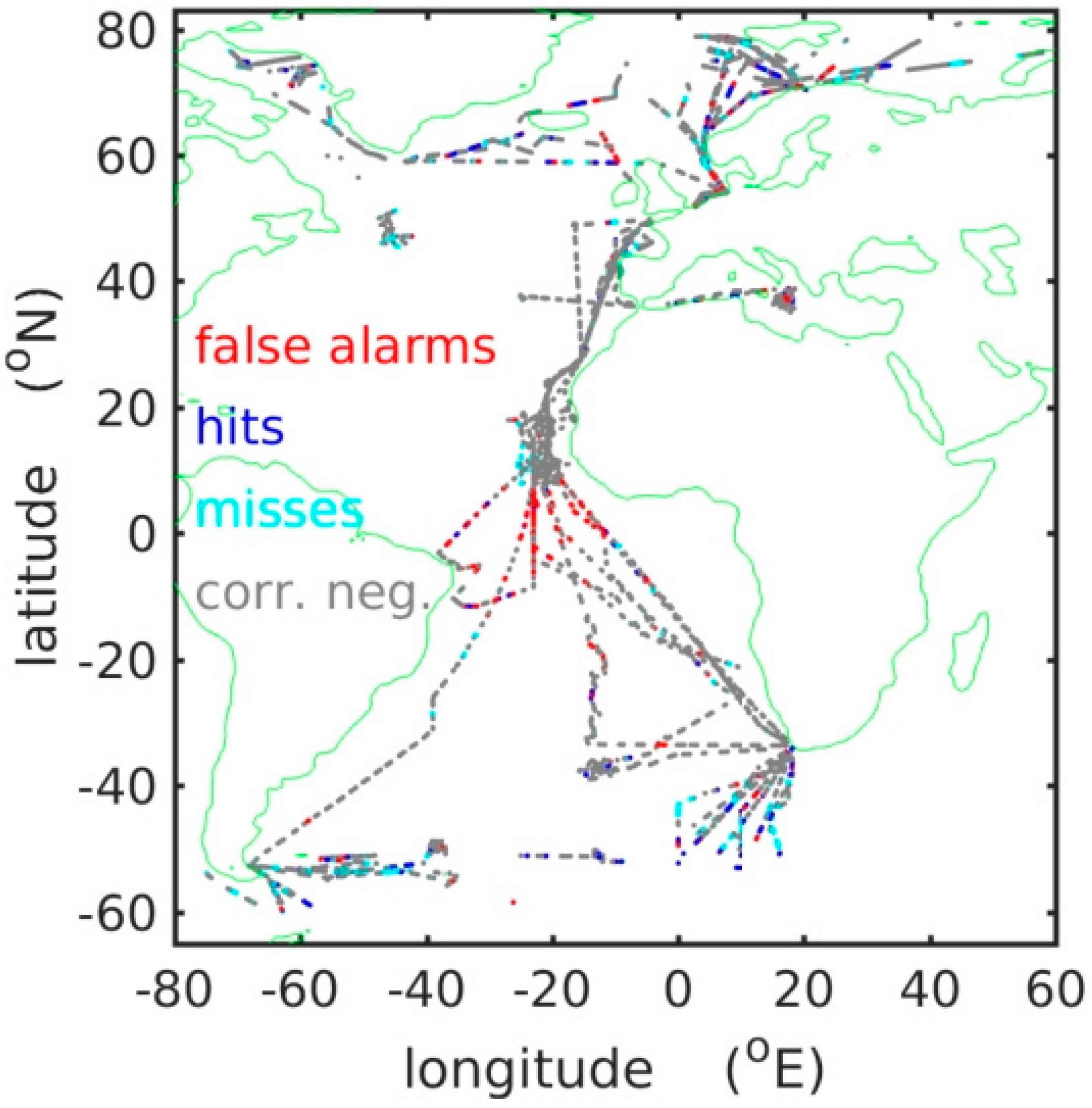
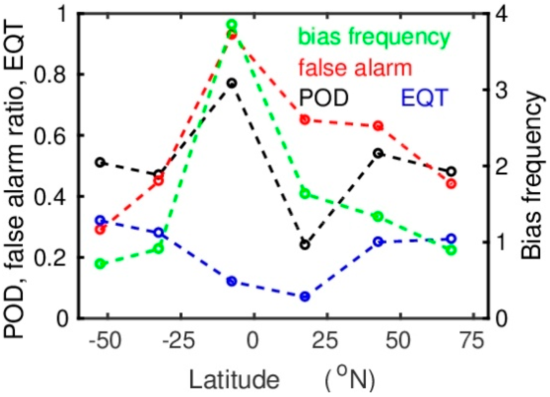
Figure 1 shows the locations of estimated hits, false alarms, misses, and correct negatives of the 2 × 2 contingency tables for each collocated event. As expected, because precipitation is a rare event, the correct negatives dominate. However, the pattern shows a concentration of false alarms especially in the vicinity of the intertropical convergence zone. This suggests that the performance of HOAPS to estimate precipitation depends on the latitude. Table 2 shows the results for six latitude belts. The coarse resolution of latitude belts is due to the limited number of collocated events. Table 2 gives the results for each ship and summarized for all ships, the latter is also seen for clarity in Figure 2. The bias frequency reached its highest values, exceeding 1, for latitudes between 20° S and 30° N, indicating that HOAPS indicates precipitation there more often than observations. Accordingly, the FAR and the POD reached high values, in which the FAR gave higher values than the POD. Combined with low values of the EQT this indicates a problem with HOAPS providing correct estimates of precipitation in the tropics. Differences between different ships were comparably small.
Table 3 provides the results for collocated events and single pairs of collocated data, the latter for two different windows in time and space used for collocation. In general, the agreement between both approaches is good. As expected, the POD increased for the events and for stricter limits of allowed temporal/spatial differences used for collocation. Unfortunately, the FARs also increased, but the increase was smaller than for the POD. The EQTs showed the highest values for stricter differences in space and time for collocation, but differences remain small. Therefore, taking into account that a reduction of allowed distances by a factor of approximately 0.5 reduces the number of collocated pairs by about 92%, the maximal differences for collocation are kept at 45 min and 55 km in the following.
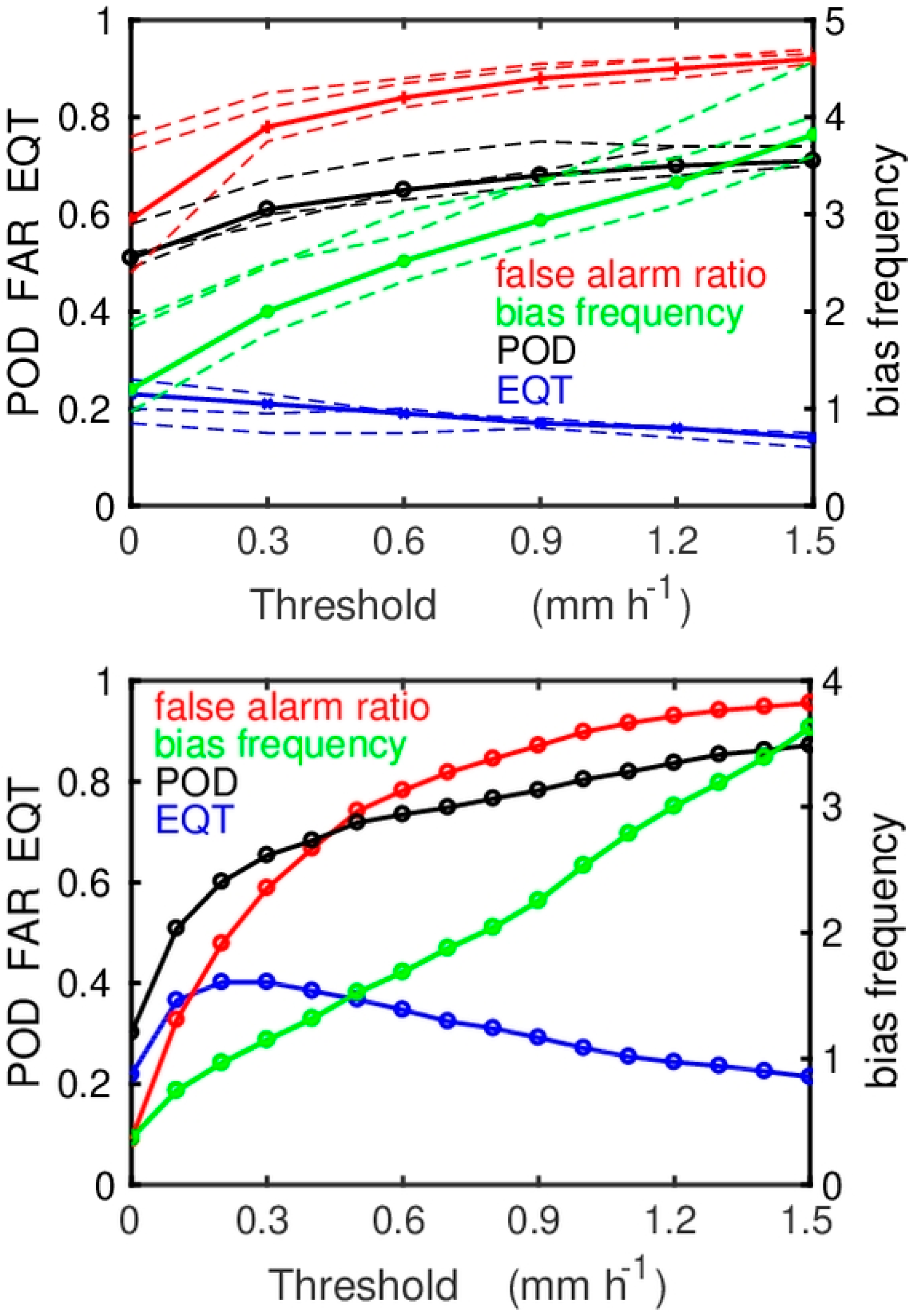
Figure 3 (top) shows how a minimum threshold applied to observations, which defines a rain/zero rain observation, influences the binary statistics. The bias frequency increases strongly with increasing threshold, which is in accordance with a moderate increase in POD, a strong increase in the FAR, and a decrease in EQT. As seen in Table 2, differences between the ships are obvious, but these were mainly caused by the fact that R/V Meteor as well as R/V Maria S. Merian measured precipitation more often in the tropics than R/V Polarstern.
Compared to theory, all values of the binary statistic except for the bias frequency are not optimal. Thus, the question arises: what can we expect, when collocating point or along track measurements with areal estimates, which are additionally hampered by the lower satellite-based threshold? Therefore, the same statistics were performed for simulated data sets (Figure 3 bottom), here restricted to latitudes south of 55° S based on R/V Polarstern data. For this calculation, simulated observations were taken randomly from the preceding 29 min of the dataset’s time window, which is used to estimate simulated areal averages comparable to HOAPS data (see Table 1). Resulting binary statistics of the simulations, except for the FAR, again showed values that are not optimal, close to those of Table 2. The results were similar for all other latitude belts (not shown). However, there were some differences between simulations and real collocated data; the bias frequency of real data was generally higher as well as higher FARs, which often exceeded the values of the PODs.
Similar to real data, with an increasing threshold applied on simulated observations, bias frequency increased rapidly as well as the FAR, while POD increased only slightly and the EQT dropped to values of less than 0.2 after a small increase to 0.38 for a threshold up to 0.3 mm·h−1.
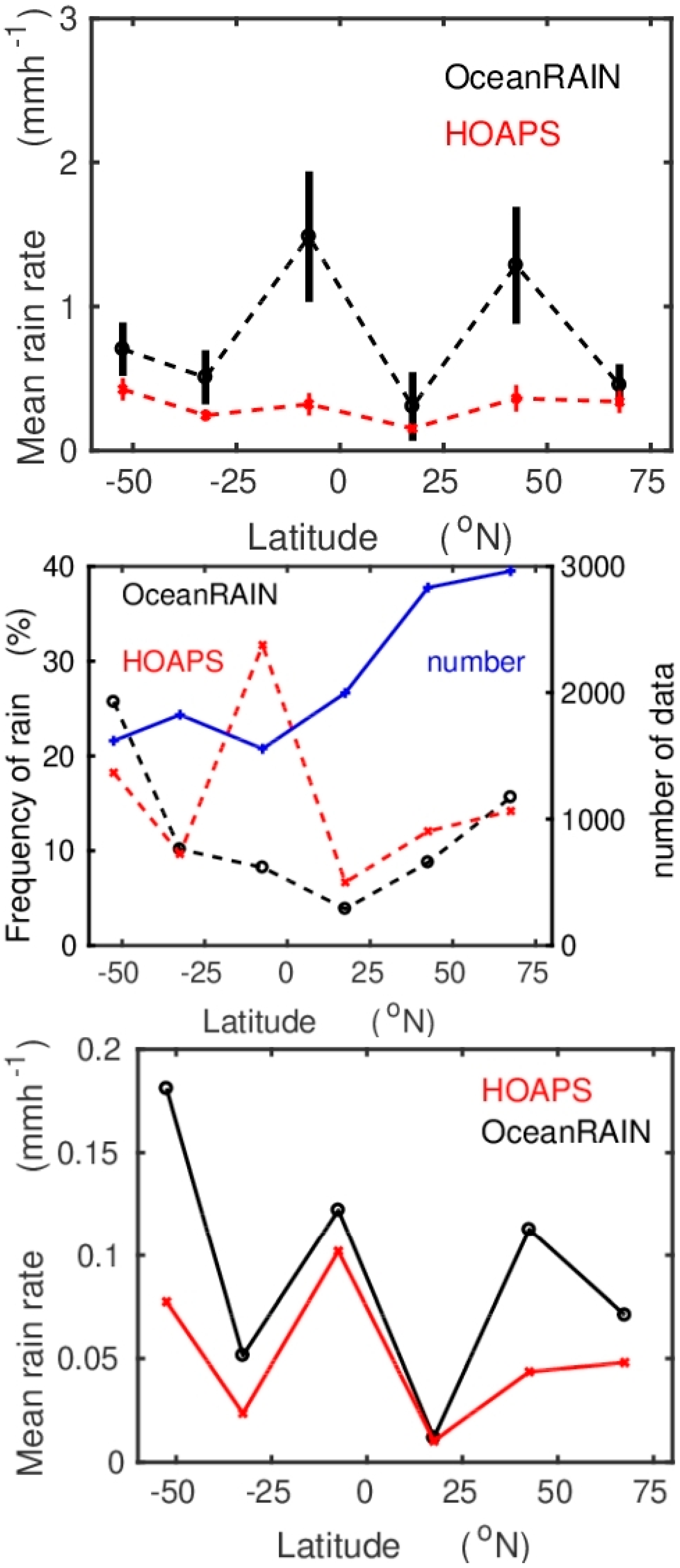
Summarized estimated numbers of binary statistics indicate a reasonable agreement between HOAPS and OceanRAIN, but there are some regional differences pointing to weaknesses in HOAPS’s performance to estimate precipitation correctly. To have a closer look at the data, the frequencies of precipitation (Figure 4 center), as well as the mean rain rates and their standard deviations for precipitating cases, were estimated for all latitude belts (Figure 4 top). Standard deviations are derived by applying the Bootstrap method [36]. The resulting average rain rates, calculated from the mean rain rate and the frequency of rain taking zero rain into account, are depicted in Figure 4 (bottom), too.
Figure 4 (center) shows that HOAPS underestimated the rain frequency in the most southern latitudes by about one third, while it overestimated the frequency considerably in the tropics compared to observations. Mean rain rates, estimated only from data with rain, were generally too small, as well as their variability. However, for latitude belts south of 20° S and north of 5° N, except for latitudes between 30° N and 55° N, estimated mean rain rates from observations and from HOAPS agree within the range of uncertainties. Taking the rain frequency into account also, HOAPS generally underestimated the observed average precipitation (Figure 4, bottom), except for the northern sub-tropics, where precipitation generally is close to zero.
Figure 5 depicts the same as Figure 4 but now derived from merged events. As expected, due to averaging, mean rain rates and their standard deviation for precipitating situations decreased for HOAPS and OceanRAIN (Figure 5 top), frequencies of rain increased (Figure 5 center), and the resulting average rain rates showed only very small changes (Figure 5 bottom), caused by differences in the data selection.
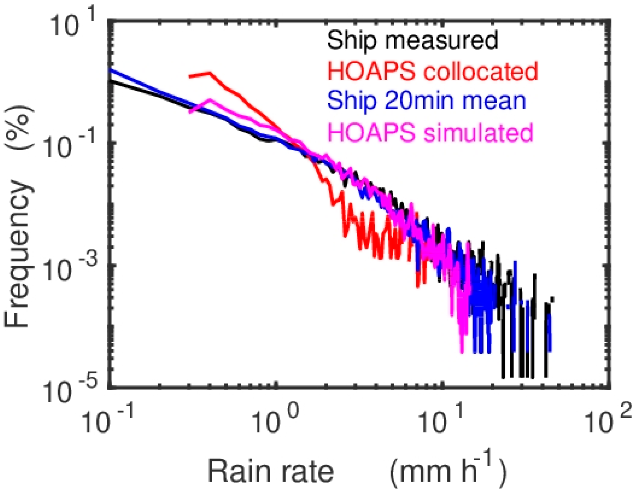
To determine possible explanations, histograms of rain rates were estimated (Figure 6) for observations and HOAPS estimates, both taken from collocated data pairs, for observed rain rates averaged over 20 min, and for simulated areal estimates derived from measured time series. Histograms show that HOAPS did not include the highest observed rain rates. However, this is expected due to spatial averaging according to the pixel size. Further, HOAPS gave less frequent moderate rain rates and more frequent low rain rates than observations. The latter can also be explained by spatial averaging due to the pixel size, but there is no reason for an underestimation of moderate rain rates. This is supported by the results based on simulations, which are, on the other hand, in good agreement with the HOAPS histogram with respect to the lowest and highest rain rates (Figure 6). The underestimation of the frequency of moderate rain rates for HOAPS estimates can explain, together with missing high and low rain rates as a consequence of averaging according to the pixel size, the smaller variability of the HOAPS estimates compared to observations. This leads to the large discrepancies found in the tropics especially, where rain rates usually are high as indicated by the observations. The 20 min averages of observations differed only a little from 1-min observations, but they also typically showed a reduction of the frequency of high rain rates and an increase of the probability of small rain rates due to temporal averaging.
5. Discussion and Conclusions
The difficulties encountered by comparing in-situ point or along-track measurements with areal averages, the latter additionally impacted by a lower satellite retrieval-based threshold, are crucial in the statistical analysis. In general, one might expect that HOAPS should detect precipitation more often than ship measurements due to its pixel size, tending to a bias score exceeding 1 and an increasing number of false alarms. However, HOAPS applies a lower threshold of 0.3 mm·h−1, a rain rate which is observed frequently in OceanRAIN (Figure 6). On the other hand, the probability of point or along-track measurements is small to meet precipitation events in an area of about 2000 km2, which is the HOAPS pixel size. All this is expressed in binary statistics, which diverge greatly from the optimum (Figure 2 and Figure 3). However, using simulated areal estimates and simulated collocated observations, derived from OceanRAIN measurements according to Section 3.3, generates numbers of binary statistics which agree nicely with results based on OceanRAIN measurements collocated with HOAPS estimates (Figure 3).
An approach to overcome problems in comparing point/along track measurements with areal averages was published by Reference [22], who developed a statistical method derived from simulations based on radar measurements over the sea to improve the validation of areal averages against point/along-track measurements. As a function of the duration of measured precipitation, they applied a procedure to transfer in a first step point measurements to areal estimates, followed by a statistical adjustment. Applying this method on the collocated OceanRAIN measurements leads to a strong decrease in mean observed precipitation rates shown in Figure 4 and Figure 5 (bottom panels), the reduction ranging from 50 to about 75% for different latitude belts, while mean HOAPS rain rates remain unchanged.
However, in principle, averaging should keep the mean value when taking all observations, with and without observed rain, into account. Taking only measurements showing rain into account, averaging should lead to an increase in lowest rain rates and a decrease in the highest measured rain rates. All this leads to a reduction in the mean rain rate of cases with rain combined with an increase in the number of rainy events. For example, the highest mean rain rate observed for latitudes between 20° S and 5° N is about 3.4 mm·h−1 based on 1-min measurements. This value is reduced to about 1.5 mm·h−1 for collocated events, which represent 30-min averages. The total rain rate of the observations, also taking all times without rain into account, is constantly 0.13 mm·h−1 in both cases (Figure 4 and Figure 5). This shows clearly that the chosen method to define events keeps the mean value, while the method of Reference [22] does not.
However, deviations may occur when the number of observations is too small. To check, whether the number of observations in our study is sufficient, the number of used collocated data pairs, which are merged to events, has been reduced by 33% and 50%. The estimated mean OceanRAIN precipitation rates remain nearly constant, changes are less than 5% compared to rain rates given in Figure 4 and Figure 5. Therefore, we conclude that, despite data sparsity from OceanRAIN, it is enough to obtain robust statistics.
Furthermore, the temporal and spatial distribution of collocated OceanRAIN observations with respect to the affiliated HOAPS pixels have been investigated. It was found that observations are equally distributed with respect to time differences to HOAPS overflight times. A regression of the number of spatial distances between the center of the HOAPS pixels and the ships’ positions gives an increase in the number of collocated measurements proportional to about 4.5 times the distance. This indicates a close to perfect spatial and temporal distribution of collocated measurements with respect to HOAPS pixels. It can be concluded that apart from the number of data, their spatial distribution is also sufficient for validation purposes.
A comparison of the ratio of the mean HOAPS rain rates to the mean OceanRAIN rain rates for the events as a function of the duration of the observed rain events gives similar results as in Reference [22], (see their Figure 4a) before they applied their suggested statistical correction procedure. There is an overestimation of rain rates by HOAPS for short rain events and an underestimation of rain rates for rain events lasting longer than about 12 min, going along with a bias (HOAPS minus OceanRAIN) of −0.64 mm·h−1 (hits only) [22]. Our analysis results in a bias of −0.57 mm·h−1, a number which is close to the reduction in observed rain rates by applying the suggested method of Reference [22].
Thus, the method to improve collocations between point measurements and areal estimates by Reference [22] seems to be some kind of adjustment of the ship measurements, which are believed to be the truth, by the radar precipitation rate estimates. Another disadvantage of the method by Reference [22] is that observations of no precipitation, which may have failed to meet existing precipitation events within the HOAPS pixel due to the small probability of rain (Figure 6), cannot be adjusted by this method at all and are kept at zero precipitation.
Therefore, we are confident that our method gives reliable results in validating HOAPS, showing that HOAPS tends to underestimate precipitation. This is supported by the histograms (Figure 6) of observations, 20 min averages of observations, HOAPS, and simulated areal averages derived from observations according to Table 1. Compared to 1 min observations 20 min averaged observations as well as simulated areal averages give the expected behavior, reducing the number of high precipitation rates and increasing the number of low precipitation rates. Comparing the HOAPS histogram with the others, it is obvious that HOAPS underestimates the probability of precipitation rates exceeding 2 mm·h−1. Results for other latitude belts are similar (not shown), with uncertainties increasing due to the lower number of collocated data.
Thus, one can conclude that HOAPS tends to underestimate rain rates due to problems in analyzing moderate to high precipitation rates. This becomes mostly obvious in areas with highest observed rain rates exceeding 40 mm·h−1, such as the intertropical convergence zone or the latitude belt from 30° N to 55° N where most data are collected in the Gulf Stream area (Figure 1), as shown in Figure 4 and Figure 5. In all other latitudes observed highest rain rates do not exceed 25 mm·h−1. The histogram (Figure 6) also explains that the lower variability of HOAPS compared to observations is not only a consequence of spatial averaging but also a consequence of missing higher precipitation rates in the HOAPS estimates. In the tropics, the low HOAPS rain rates were in parts compensated by a very high frequency of precipitating situations in the HOAPS retrievals. It might be speculated that this is probably caused by the size of cloud clusters and the high precipitation rates, which in combination with the HOAPS pixel size force an exceedance of the lower threshold.
The results are comparable to an earlier study [31], comparing ship rain gauge measurements of the period from 2005–2008 with an earlier version of HOAPS precipitation estimates. The main results of the former study were a strong underestimation of the mean rain rates south of 30° S and north of 40° N and a high rate of false alarms in the tropics. The present study, using OceanRAIN, comprises about five times more collocated data, which enables a closer look at the details. Thus, it was found that the strong underestimation at higher latitudes is mainly caused by an underestimation of rain rates by HOAPS, while the frequency of rain is well represented. In the present study, we find that such an underestimation of rain rates also occurs in tropical areas, where even the strong overestimation in the frequency of rain by HOAPS, also seen in the former study [31], does not balance this deficit.
In addition, other HOAPS satellite products are available. For the future, we plan to validate the GPM (from 2014 onwards) and TRMM data sets (1997–2015). The newly developed collocation software, used within the present study, also allows the collocation of these data sets. However, the available periods of these data differ from the period where HOAPS data are available.
Ongoing measurements within OceanRAIN will broaden the database in the future. However, even long time series will not solve a general problem; ship measurements do not cover all areas all over the year. For example, measurements at high latitudes are usually only available during the summer months, although OceanRAIN also provides some Antarctic winter snowfall data. Thus, in-situ data cannot reach the spatio-temporal coverage of satellite-based data sets. However, a project, such as OceanRAIN, provides comprehensive data sets, which can serve as reference data for satellite-derived precipitation data, enabling validation studies, such as the one in the present paper.
Author Contributions
Conceptualization, K.B. and M.S.; Data curation, C.K. and K.F.; Formal analysis, K.B. and R.P.K.; Funding acquisition, K.B. and M.S.; Methodology, K.B.; Project administration, K.B. and M.S.; Software, K.B. and R.P.K.; Writing—original draft, K.B.; Writing—review and editing, R.P.K., M.S., C.K. and K.F.
Funding
The development of the collocation software was funded by the German Weather Service, precipitationW.
Acknowledgments
Meteorological data of R/V Maria S. Merian are provided from the DOD (Deutsches Ozeanographisches Datenzentrum) maintained by the Bundesamt für Seeschifffahrt und Hydrographie. Our thanks also go to Kathrin Graw, who organized the data exchange with the DWD. We would like to thank also the four reviewers, whose valuable suggestions and comments helped us to improve the paper.
Conflicts of Interest
The authors declare no conflict of interest. The funders had no role in the design of the study; in the collection, analyses, or interpretation of data; in the writing of the manuscript, or in the decision to publish the results.
References
- Schmitt, R.W. Salinity and the global water cycle. Oceanography 2008, 21, 12–19. [Google Scholar] [CrossRef]
- Rhein, M.; Rintoul, S.R.; Aoki, S.; Campos, E.; Chambers, D.; Feely, R.A.; Gulev, S.; Johnson, G.C.; Josey, S.A.; Kostianoy, A.; et al. Observations: Ocean. In Climate Change 2013: The Physical Science Basis, Contribution of Working Group I to the Fifth Assessment Report of the Intergovernmental Panel on Climate Change; Stocker, T.F., Qin, D., Plattner, G.-K., Tignor, M., Allen, S.K., Boschung, J., Nauels, A., Xia, Y., Bex, V., Midgley, P.M., Eds.; Cambridge University Press: Cambridge, UK; New York, NY, USA, 2013; pp. 659–740. [Google Scholar] [CrossRef]
- Andersson, A.; Graw, K.; Schröder, M.; Fennig, K.; Liman, J.; Bakan, S.; Hollmann, R.; Klepp, C. Hamburg Ocean Atmosphere Parameters and Fluxes from Satellite Data—HOAPS 4.0. 2017. Available online: https://wui.cmsaf.eu/safira/action/viewDoiDetails?acronym=HOAPS_V002 (accessed on 8 November 2018).
- Hou, A.Y.; Kakar, R.K.; Neeck, S.; Azarbarzin, A.A.; Kummerow, C.D.; Kojima, M.; Oki, R.; Nakamura, K.; Iguchi, T. The Global Precipitation Measurement Mission. Bull. Am. Meteorol. Soc. 2014, 95, 701–722. [Google Scholar] [CrossRef] [Green Version]
- Huffman, G.J.; Adler, R.F.; Bolvin, D.T.; Gu, G.; Nelkin, E.J.; Bowman, K.P.; Hong, Y.; Stocker, E.F.; Wolff, D.B. The TRMM Multi-satellite Precipitation Analysis: Quasi-Global, Multi-Year, Combined-Sensor Precipitation Estimates at Fine Scale. J. Hydrometeorol. 2007, 8, 38–55. [Google Scholar] [CrossRef]
- Dee, D.P.; Uppala, S.M.; Simmons, A.J.; Berrisford, P.; Poli, P.; Kobayashi, S.; Andrae, U.; Balmaseda, M.A.; Balsamo, G.; Bauer, P.; et al. The ERA-Interim reanalysis: Configuration and performance of the data assimilation system. Q. J. R. Meteorol. Soc. 2011, 137, 553–597. [Google Scholar] [CrossRef]
- HOAPS. Available online: http://www.hoaps.org (accessed on 11 December 2018).
- NASA. Available online: https://pmm.nasa.gov/data-access/downloads/trmm (accessed on 11 December 2018).
- NASA. Available online: https://pmm.nasa.gov/data-access/downloads/gpm (accessed on 11 December 2018).
- Sanò, P.; Panegrossi, G.; Casella, D.; Marra, A.C.; Di Paola, F.; Dietrich, S. The new Passive microwave Neural network Precipitation Retrieval (PNPR) algorithm for the cross-track scanning ATMS radiometer: Description and verification study over Europe and Africa using GPM and TRMM spaceborne radars. Atmos. Meas. Tech. 2016, 9, 5441–5460. [Google Scholar] [CrossRef]
- Andersson, A.; Klepp, C.; Fennig, K.; Bakan, S.; Graßl, H.; Schulz, J. Evaluation of HOAPS-3 ocean surface freshwater flux components. J. Appl. Meteorol. Climatol. 2011, 50, 379–398. [Google Scholar] [CrossRef]
- Pfeifroth, U.; Mueller, R.; Ahrens, B. Evaluation of Satellite-Based and Reanalysis Precipitation Data in the Tropical Pacific. J. Appl. Meteorol. Climatol. 2013, 52, 634–644. [Google Scholar] [CrossRef]
- Huffman, G.J.; Adler, R.F.; Bolvin, D.T.; Gu, G. Improving the Global Precipitation Record: GPCP Version 2.1. Geophys. Res. Lett. 2009, 36, L17808. [Google Scholar] [CrossRef]
- Schlosser, C.A.; Houser, P.R. Assessing a Satellite-era Perspective of the Global Water Cycle. J. Clim. 2007, 20, 1316–1338. [Google Scholar] [CrossRef]
- Prakash, S.; Gairola, R.M. Validation of Trmm-3b42 Precipitation Product Over the Tropical Indian Ocean Using Rain Gauge Data from the Rama Buoy Array. Theor. Appl. Climatol. 2014, 115, 451–460. [Google Scholar] [CrossRef]
- Huffman, G.J.; Adler, R.F.; Bolvin, D.T.; Nelkin, E.J. The TRMM Multi-satellite Precipitation Analysis (TMPA). In Satellite Applications for Surface Hydrology; Hossain, F., Gebremichael, M., Eds.; Springer: Berlin, Germany, 2010; pp. 3–22. ISBN 978-90-481-2914-0. [Google Scholar]
- Neiman, P.J.; Gaggini, N.; Fairall, C.W.; Aikins, J.; Spackman, J.R.; Leung, L.R.; Fan, J.; Hardin, J.; Nalli, N.R.; White, A.B. An analysis of coordinated observations from NOAA’s Ronald H. Brown Ship and G-IV aircraft in a landfalling atmospheric river over the North Pacific, during CalWater-2015. Mon. Weather Rev. 2017, 145, 3647–3669. [Google Scholar] [CrossRef]
- Klepp, C. The oceanic shipboard precipitation measurement network for surface validation–OceanRAIN. Atmos. Res. 2015, 163, 74–90. [Google Scholar] [CrossRef]
- Klepp, C.; Michel, S.; Protat, A.; Burdanowitz, J.; Albern, N.; Dahl, A.; Kähnert, M.; Louf, V.; Bakan, S.; Buehler, S.A. OceanRAIN, a new in-situ shipboard global ocean surface-reference dataset of all water cycle components. Sci. Data 2018, 5. [Google Scholar] [CrossRef] [PubMed]
- Großklaus, M.; Uhlig, K.; Hasse, L. An optical disdrometer for use in high wind speeds. J. Atmos. Ocean. Technol. 1998, 15, 1051–1059. [Google Scholar] [CrossRef]
- Klepp, C.; Michel, S.; Protat, A.; Burdanowitz, J.; Albern, N.; Louf, V.; Bakan, S.; Dahl, A.; Thiele, T. Ocean Rainfall and Ice-Phase Precipitation Measurement Network—OceanRAIN-W; World Data Center for Climate (WDCC) at DKRZ: Hamburg, Germany, 2017. [Google Scholar]
- Burdanowitz, J.; Klepp, C.; Bakan, S.; Buehler, S.A. Simulation of Ship-Track versus Satellite-Sensor Differences in Oceanic Precipitation Using an Island-Based Radar. Remote Sens. 2017, 9, 593. [Google Scholar] [CrossRef]
- DWD. Available online: https://www.dwd.de/DE/fachnutzer/forschung_lehre/numerische_wettervorhersage/nwv_aenderungen/_functions/DownloadBox_modellaenderungen/cosmo_d2/pdf_2018_2020/pdf_cosmo_d2_15_05_2018.html?nn=346850 (accessed on 11 December 2018).
- Andersson, A.; Fennig, K.; Klepp, C.; Bakan, S.; Graßl, H.; Schulz, J. The Hamburg Ocean Atmosphere Parameters and Fluxes from Satellite Data—HOAPS-3. Earth Syst. Sci. Data 2010, 2, 215–234. [Google Scholar] [CrossRef]
- Fennig, K.; Andersson, A.; Bakan, S.; Klepp, C.P.; Schröder, M. Hamburg Ocean Atmosphere Parameters and Fluxes from Satellite Data—HOAPS 3.2—Monthly Means/6-Hourly Composites; Satellite Application Facility on Climate Monitoring (CM SAF): Geneva, Switzerland, 2012. [Google Scholar] [CrossRef]
- Bauer, P.; Lopez, P.; Benedetti, A.; Salmond, D.; Moreau, E. Implementation of 1D+4D-var assimilation of precipitation-affected microwave radiances at ECMWF: 1D-var. Q. J. R. Meteorol. Soc. 2006, 132, 2277–2306. [Google Scholar] [CrossRef]
- Bauer, P.; Moreau, E.; Chevallier, F.; O’Keeffe, U. Multiplescattering microwave radiative transfer for data assimilation applications. Q. J. R. Meteorol. Soc. 2006, 132, 1259–1281. [Google Scholar] [CrossRef]
- Froidurot, S.; Zin, I.; Hingray, B.; Gautheron, A. Sensitivity of Precipitation Phase over the Swiss Alps to Different Meteorological Variables. J. Hydrometeorol. 2014, 15, 685–696. [Google Scholar] [CrossRef]
- Hasse, L.; Großklaus, M.; Uhlig, K.; Timm, P. A ship rain gauge for use under high wind speeds. J. Atmos. Ocean. Technol. 1998, 15, 380–386. [Google Scholar] [CrossRef]
- Bundesamt für Seeschifffahrt und Hydrographie (BSH), DOD Data Centre. 2015. Available online: http://www.bsh.de/en/Marine_data/Observations/DOD_Data_Centre/ (accessed on 8 November 2018).
- Bumke, K.; König-Langlo, G.; Kinzel, J.; Schröder, M. HOAPS and ERA-Interim precipitation over the sea: Validation against shipboard in situ measurements. Atmos. Meas. Tech. 2016, 9, 1–15. [Google Scholar] [CrossRef]
- Clemens, M.; Bumke, K. Precipitation fields over the Baltic Sea derived from ship rain gauge measurements on merchant ships. Boreal Environ. Res. 2002, 7, 425–436. [Google Scholar]
- Klepp, C.; Bumke, K.; Bakan, S.; Bauer, P. Ground validation of oceanic snowfall detection in satellite climatologies during LOFZY. Tellus A Dyn. Meteorol. Oceanogr. 2010, 62, 469–480. [Google Scholar] [CrossRef] [Green Version]
- WWRP/WGNE. Methods for Dichotomous Forecasts. Joint Working Group on Verification Sponsored by the WMO, Forecast Verification, Issues, Methods and FAQ. Available online: www.cawcr.gov.au/projects/verification/#Methods_for_dichotomous_forecasts (accessed on 11 September 2018).
- Bumke, K.; Karger, U.; Hasse, L.; Niekamp, K.-P. Evaporation over the Baltic Sea as an example of a semi-enclosed sea. Contrib. Atmos. Phys. 1998, 71, 249–261. [Google Scholar]
- Efron, B. Bootstrap Methods: Another Look at the Jackknife. Ann. Stat. 1979, 7, 1–26. [Google Scholar] [CrossRef]
Figure 1.
Locations of collocated data of ship measurements and HOAPS (Hamburg Ocean Atmosphere Parameters and Fluxes from Satellite Data) data merged to events. Colors indicate the results in terms of false alarms, hits, misses and correct negatives for each event used to build the 2 × 2 contingency table.

Figure 2.
Results of the binary statistic applied on collocated data events for latitude belts south of 45° S, 45° S–20° S, 20° S–5° N, 5° N–30° N, 30° N–55° N, and north of 55° N.
Figure 2.
Results of the binary statistic applied on collocated data events for latitude belts south of 45° S, 45° S–20° S, 20° S–5° N, 5° N–30° N, 30° N–55° N, and north of 55° N.

Figure 3.
Top: Results of the binary statistic applied on collocated data events of all data (solid lines) and separately for R/Vs Polarstern, Meteor, and Maria S. Merian (dashed lines) as a function of a lower threshold applied on observations. Data of all latitudes were used. Bottom: Results of the binary statistic applied on collocated pairs of simulated data as a function of a lower threshold applied on observations. Simulated data are based on R/V Polarstern measurements south of 45° S.

Figure 4.
Mean rain rates and their standard deviation derived only from data with precipitation (top), frequency of rain and number of data (center) and resulting mean rain rates (bottom) estimated from collocated pairs of OceanRAIN (Ocean Rainfall And Ice-phase precipitation measurement Network) observations and HOAPS data taking zero values separately into account.

Figure 5.
Mean rain rates and their standard deviation derived only from data with precipitation (top), frequency of rain and number of data (center) and resulting mean rain rates (bottom) estimated for collocated data events merged from collocated pairs of OceanRAIN observations and HOAPS data taking zero values separately into account.

Figure 6.
Histogram of rain rates (0.1 mm·h−1 increments) in terms of frequency for collocated ship measurements and HOAPS data as well as for 20 min averages of measurements and simulated HOAPS data derived from time series of measurements. Data of all latitudes are used.
Figure 6.
Histogram of rain rates (0.1 mm·h−1 increments) in terms of frequency for collocated ship measurements and HOAPS data as well as for 20 min averages of measurements and simulated HOAPS data derived from time series of measurements. Data of all latitudes are used.


Table 1.
Scheme for simulating areal means from a time series. Numbers indicate the element of the time series.
Table 1.
Scheme for simulating areal means from a time series. Numbers indicate the element of the time series.
| 3 | 2 | 1 | 2 | 3 |
| 4 | 3 | 2 | 3 | 4 |
| 5 | 4 | 3 | 4 | 5 |
| 6 | 5 | 4 | 5 | 6 |
| 7 | 6 | 5 | 6 | 7 |
Table 2.
Probability of detection (POD), bias score, false alarm ratio (FAR), and Equitable threat score (EQT) for R/V Polarstern, R/V Maria S. Merian, R/V Meteor, and based on data of all ships as a function of latitude. Statistics are based on collocated data merged to events. If there are less than 30 events with precipitation, no statistics were estimated.
| Latitude | <45° S | 45° S–20° S | 20° S–5° N | 5° N–30° N | 30° N–55° N | >55° N |
|---|---|---|---|---|---|---|
| Polarstern | ||||||
| Number | 1606 | 1159 | 716 | 736 | 936 | 2612 |
| POD | 0.51 | 0.43 | 0.64 | 0.73 | 0.50 | 0.47 |
| Bias frequ. | 0.71 | 0.71 | 3.29 | 4.91 | 1.30 | 0.83 |
| FAR | 0.29 | 0.33 | 0.88 | 0.94 | 0.62 | 0.41 |
| EQT | 0.32 | 0.28 | 0.11 | 0.13 | 0.22 | 0.27 |
| M.S.Merian | ||||||
| Number | 673 | 428 | 343 | 235 | 340 | |
| POD | 0.65 | - | - | - | 0.56 | |
| Bias frequ. | 1.70 | - | - | - | 1.34 | |
| FAR | 0.75 | - | - | - | 0.64 | |
| EQT | 0.28 | - | - | - | 0.22 | |
| Meteor | ||||||
| Number | 421 | 920 | 1666 | |||
| POD | 0.92 | - | 0.70 | |||
| Bias frequ. | 4.42 | - | 1.68 | |||
| FAR | 0.98 | - | 0.77 | |||
| EQT | 0.10 | - | 0.31 | |||
| All ships | ||||||
| Number | 1606 | 1832 | 1565 | 1999 | 2837 | 2952 |
| POD | 0.51 | 0.47 | 0.77 | 0.24 | 0.54 | 0.48 |
| Bias frequ. | 0.71 | 0.91 | 3.85 | 1.63 | 1.33 | 0.89 |
| FAR | 0.29 | 0.45 | 0.93 | 0.65 | 0.63 | 0.44 |
| EQT | 0.32 | 0.28 | 0.12 | 0.07 | 0.25 | 0.26 |
Table 3.
POD, bias score, FAR, and EQT based on data of all ships. Statistics are given for collocated data merged to events as well as all collocated pairs of data, the latter for two different maximum distances between observation and satellite’s footprint and maximum differences in time between observation and satellite used for collocation.
| All Ships, All Latitudes | Events | Collocated Pairs of Data | |
|---|---|---|---|
| Δx < 55 km, Δt < 45 min | Δx < 55 km, Δt < 45 min | Δx < 25 km, Δt < 15 min | |
| Number | 12,791 | 6,828,198 | 446,980 |
| POD | 0.51 | 0.40 | 0.47 |
| Bias frequency | 1.20 | 0.97 | 1.01 |
| FAR | 0.59 | 0.49 | 0.51 |
| EQT | 0.23 | 0.23 | 0.27 |
© 2019 by the authors. Licensee MDPI, Basel, Switzerland. This article is an open access article distributed under the terms and conditions of the Creative Commons Attribution (CC BY) license (http://creativecommons.org/licenses/by/4.0/).
Share and Cite
MDPI and ACS Style
Bumke, K.; Pilch Kedzierski, R.; Schröder, M.; Klepp, C.; Fennig, K. Validation of HOAPS Rain Retrievals against OceanRAIN In-Situ Measurements over the Atlantic Ocean. Atmosphere 2019, 10, 15. https://doi.org/10.3390/atmos10010015
AMA Style
Bumke K, Pilch Kedzierski R, Schröder M, Klepp C, Fennig K. Validation of HOAPS Rain Retrievals against OceanRAIN In-Situ Measurements over the Atlantic Ocean. Atmosphere. 2019; 10(1):15. https://doi.org/10.3390/atmos10010015
Chicago/Turabian StyleBumke, Karl, Robin Pilch Kedzierski, Marc Schröder, Christian Klepp, and Karsten Fennig. 2019. "Validation of HOAPS Rain Retrievals against OceanRAIN In-Situ Measurements over the Atlantic Ocean" Atmosphere 10, no. 1: 15. https://doi.org/10.3390/atmos10010015
Note that from the first issue of 2016, this journal uses article numbers instead of page numbers. See further details here.