
Analysis of Urban Drainage Networks Using Gibbs’ Model: A Case Study in Seoul, South Korea


Abstract
:1. Introduction
2. Methods
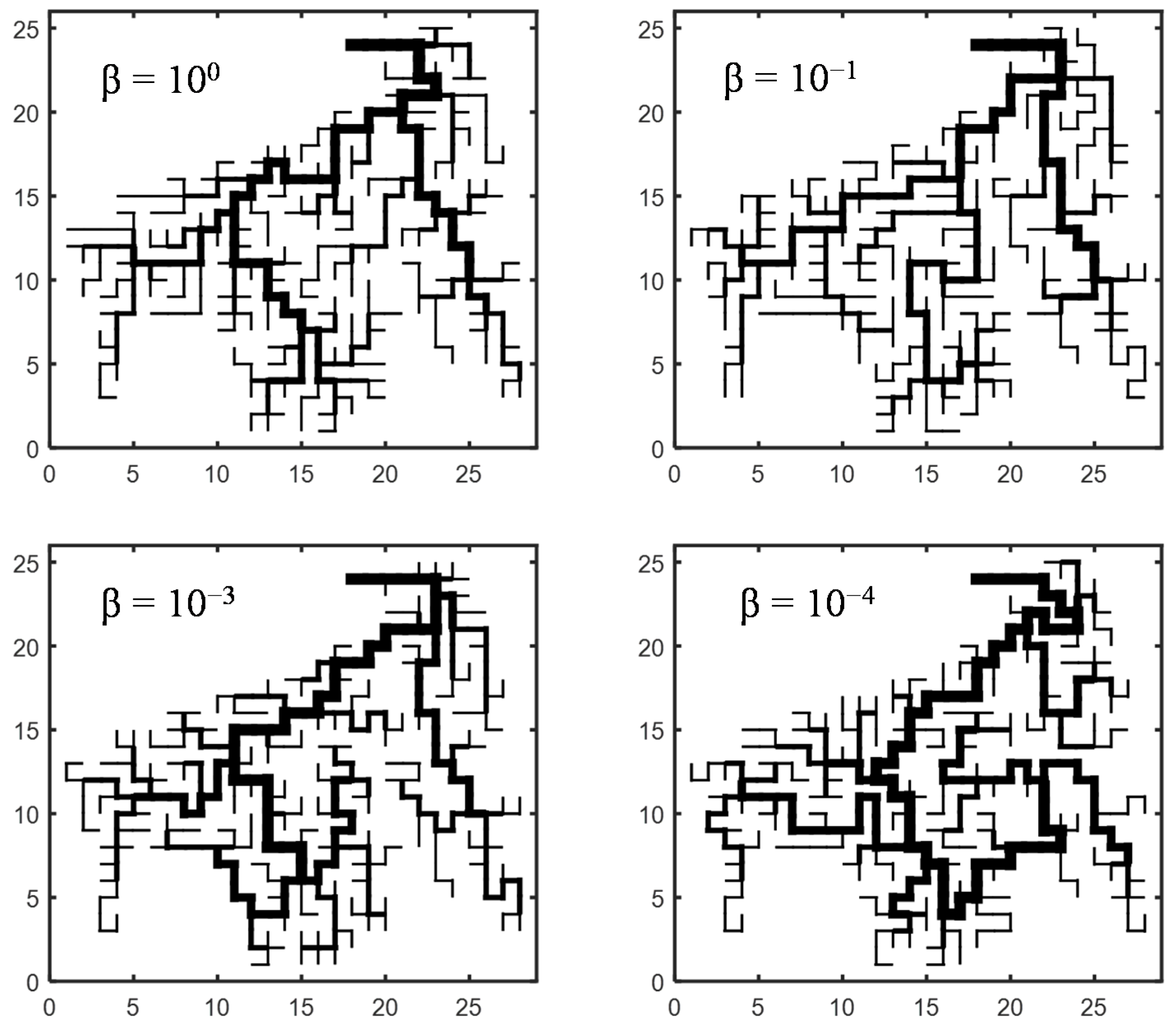
2.1. Gibbs’ Model


2.2. Study Area and Estimation of Beta


| No | ID | Catchment | Area (Aw) | Perimeter (Bp) | Drainage Density (D) | Conduit Slope (Sp) | Catchment Slope (Sc) |
|---|---|---|---|---|---|---|---|
| km2 | km | m/m2 | % | % | |||
| 1 | NH | Nonhyeon | 1.80 | 8.24 | 0.028 | 5.633 | 6.959 |
| 2 | DR | Daelim | 1.25 | 5.92 | 0.024 | 3.565 | 3.721 |
| 3 | DO | Daebang | 2.02 | 8.09 | 0.026 | 3.430 | 4.733 |
| 4 | DG | Dogok | 1.82 | 7.33 | 0.022 | 3.377 | 4.330 |
| 5 | DLO | Dorim1 | 2.71 | 9.10 | 0.037 | 0.668 | 2.921 |
| 6 | DCW | Deungchon2 | 0.87 | 4.57 | 0.022 | 5.638 | 8.461 |
| 7 | BBW | Bangbae2 | 1.37 | 7.62 | 0.026 | 4.107 | 9.395 |
| 8 | BBT | Bangbae3 | 1.66 | 7.31 | 0.011 | 6.270 | 17.273 |
| 9 | BBF | Bangbae4 | 1.56 | 7.05 | 0.010 | 5.382 | 17.392 |
| 10 | SD | Sadang | 1.83 | 6.81 | 0.021 | 4.448 | 11.364 |
| 11 | SSO | Samsung1 | 1.91 | 7.98 | 0.026 | 3.784 | 4.850 |
| 12 | SSW | Samdung2 | 2.10 | 6.88 | 0.021 | 3.076 | 5.822 |
| 13 | SDW | Sangdo2 | 1.94 | 7.76 | 0.028 | 3.321 | 9.451 |
| 14 | SCO | Seocho1 | 1.89 | 8.59 | 0.019 | 4.801 | 7.846 |
| 15 | SCT | Seocho3 | 1.79 | 8.69 | 0.017 | 3.437 | 6.959 |
| 16 | SCF | Seocho4 | 1.06 | 6.06 | 0.024 | 3.126 | 3.112 |
| 17 | SH | Shiheunggoji | 1.60 | 8.61 | 0.022 | 4.604 | 10.007 |
| 18 | SLA | Sillim1 | 1.98 | 8.84 | 0.033 | 4.489 | 9.503 |
| 19 | SLW | Sillim2 | 4.35 | 10.56 | 0.012 | 5.670 | 18.232 |
| 20 | SLM | Sillim3 | 1.36 | 5.82 | 0.019 | 6.996 | 19.319 |
| 21 | SLF | Sillim4_1 | 0.32 | 2.71 | 0.033 | 1.408 | 3.221 |
| 22 | SLF | Sillim4_2 | 2.23 | 9.08 | 0.025 | 3.342 | 9.953 |
| 23 | SWO | Sinwol1 | 1.52 | 7.46 | 0.025 | 2.663 | 5.205 |
| 24 | SWT | Sinwol3_1 | 1.20 | 5.77 | 0.035 | 2.345 | 3.014 |
| 25 | SWT | Sinwol3_2 | 0.52 | 3.48 | 0.027 | 2.540 | 3.539 |
| 26 | YS | Yeoksam | 1.93 | 7.40 | 0.030 | 3.637 | 4.996 |
| 27 | LM | Yimok | 2.09 | 8.37 | 0.023 | 5.372 | 11.820 |
| 28 | IS | Yisu | 1.37 | 5.62 | 0.024 | 4.211 | 10.168 |
| 29 | HGO | Hwagok1 | 2.28 | 7.22 | 0.025 | 4.404 | 9.820 |
| 30 | HKW | Hwagok2 | 3.26 | 10.07 | 0.029 | 3.969 | 6.243 |
| 31 | HY | Hyoja | 5.43 | 10.97 | 0.016 | 4.263 | 16.030 |

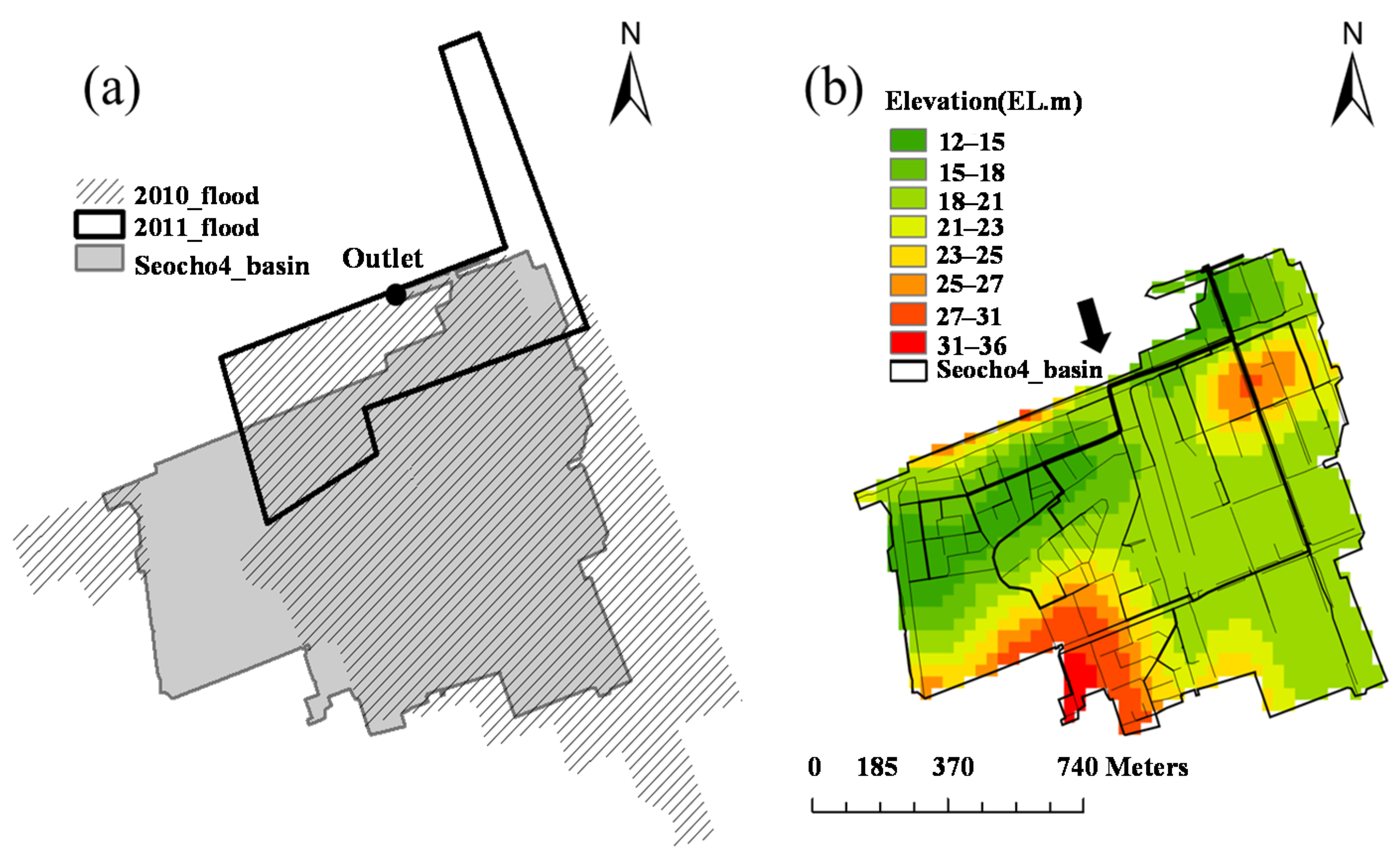
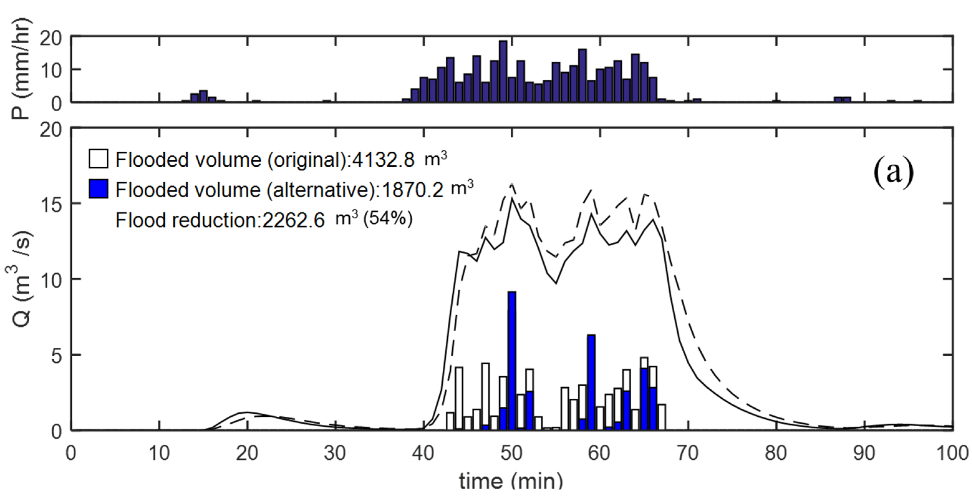
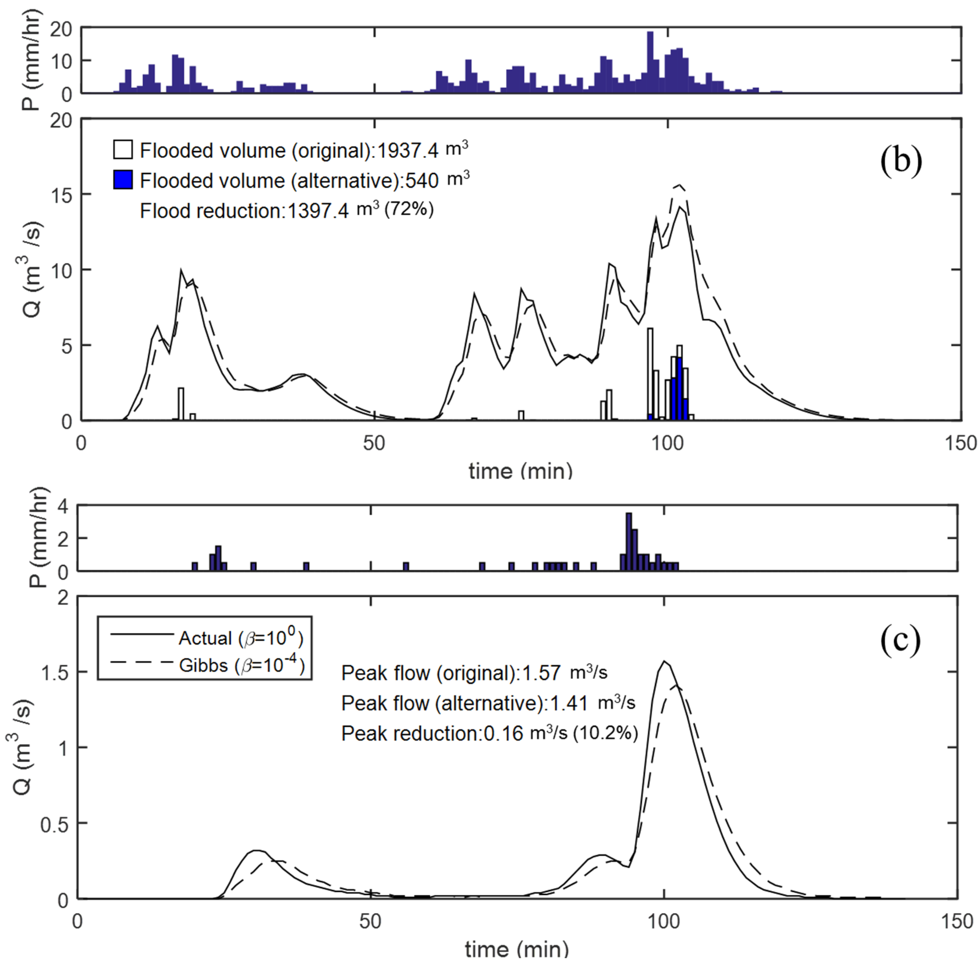
2.3. Flood in 2010 and 2011 in a Test Catchment, Seocho4

3. Results and Discussion
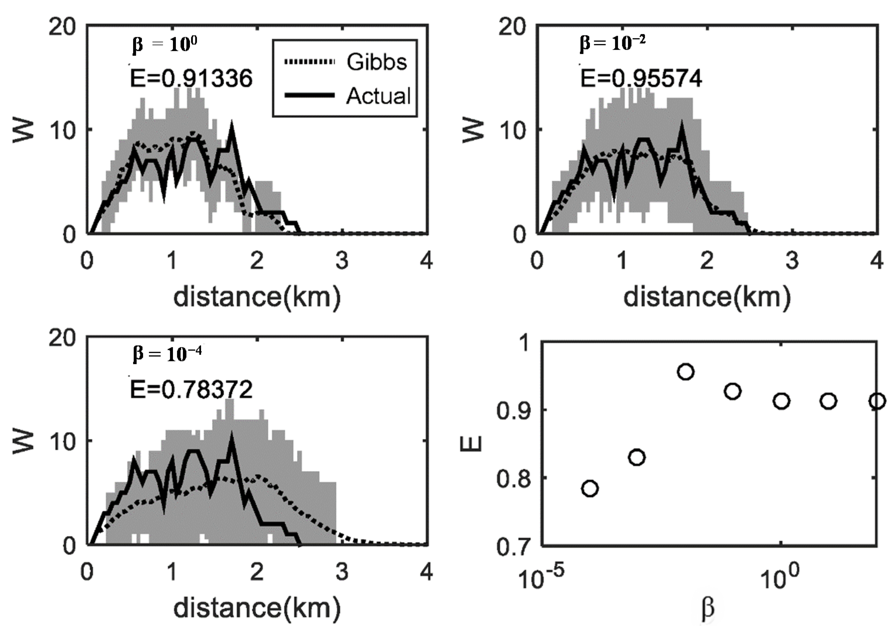
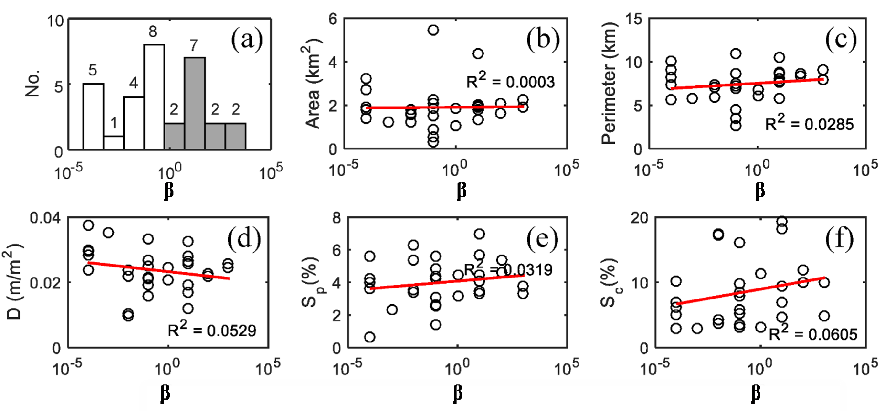
3.1. Network Configuration of Urban Catchments in Seoul
| No | ID | Catchment | Basin Area (Aw) | Grid Size | n | m | Goodness of Fit (E) | O(β) |
|---|---|---|---|---|---|---|---|---|
| km2 | m | |||||||
| 1 | NH | NonHyeon | 1.80 | 50 | 43 | 34 | 0.77 | 10−4 |
| 2 | DR | DaeLim | 1.25 | 50 | 24 | 27 | 0.91 | 10−2 |
| 3 | DO | DaeBang | 2.02 | 50 | 34 | 39 | 0.62 | 101 |
| 4 | DG | DoGok | 1.82 | 50 | 27 | 42 | 0.70 | 10−2 |
| 5 | DLO | DoRim1 | 2.71 | 50 | 48 | 36 | 0.52 | 10−4 |
| 6 | DCW | DeungChon2 | 0.87 | 50 | 22 | 21 | 0.99 | 10−1 |
| 7 | BBW | BangBae2 | 1.37 | 50 | 41 | 27 | 0.91 | 101 |
| 8 | BBT | BangBae3 | 1.66 | 50 | 21 | 31 | 0.96 | 10−2 |
| 9 | BBF | BangBae4 | 1.56 | 50 | 25 | 26 | 0.96 | 10−2 |
| 10 | SD | SaDang | 1.83 | 50 | 30 | 23 | 0.82 | 100 |
| 11 | SSO | SamSung1 | 1.91 | 50 | 36 | 38 | 0.87 | 103 |
| 12 | SSW | SamDung2 | 2.10 | 50 | 41 | 33 | 0.87 | 10−1 |
| 13 | SDW | SangDo2 | 1.94 | 50 | 33 | 38 | 0.93 | 101 |
| 14 | SCO | SeoCho1 | 1.89 | 50 | 47 | 36 | 0.73 | 10−1 |
| 15 | SCT | SeoCho3 | 1.79 | 50 | 28 | 40 | 0.79 | 101 |
| 16 | SCF | SeoCho4 | 1.06 | 50 | 25 | 28 | 0.96 | 100 |
| 17 | SH | ShiHeungGoJi | 1.60 | 50 | 49 | 36 | 0.88 | 102 |
| 18 | SLA | SilLim1 | 1.98 | 50 | 42 | 42 | 0.71 | 101 |
| 19 | SLW | SilLim2 | 4.35 | 50 | 34 | 44 | 0.89 | 101 |
| 20 | SLM | SilLim3 | 1.36 | 50 | 36 | 22 | 0.92 | 101 |
| 21 | SLF | SilLim4_1 | 0.32 | 50 | 12 | 13 | 0.99 | 10−1 |
| 22 | SLF | SilLim4_2 | 2.23 | 50 | 46 | 30 | 0.77 | 103 |
| 23 | SWO | Sinwol1 | 1.52 | 50 | 31 | 24 | 0.85 | 10−1 |
| 24 | SWT | Sinwol3_1 | 1.20 | 50 | 24 | 32 | 0.80 | 10−3 |
| 25 | SWT | Sinwol3_2 | 0.52 | 50 | 15 | 22 | 0.93 | 10−1 |
| 26 | YS | YeokSam | 1.93 | 50 | 33 | 35 | 0.78 | 10−4 |
| 27 | LM | YiMok | 2.09 | 50 | 39 | 42 | 0.80 | 102 |
| 28 | IS | YiSu | 1.37 | 50 | 37 | 24 | 0.73 | 10−4 |
| 29 | HGO | HwaGok1 | 2.28 | 50 | 38 | 30 | 0.88 | 101 |
| 30 | HKW | HwaGok2 | 3.26 | 50 | 43 | 40 | 0.76 | 10−4 |
| 31 | HY | HyoJa | 5.43 | 50 | 56 | 46 | 0.70 | 101 |

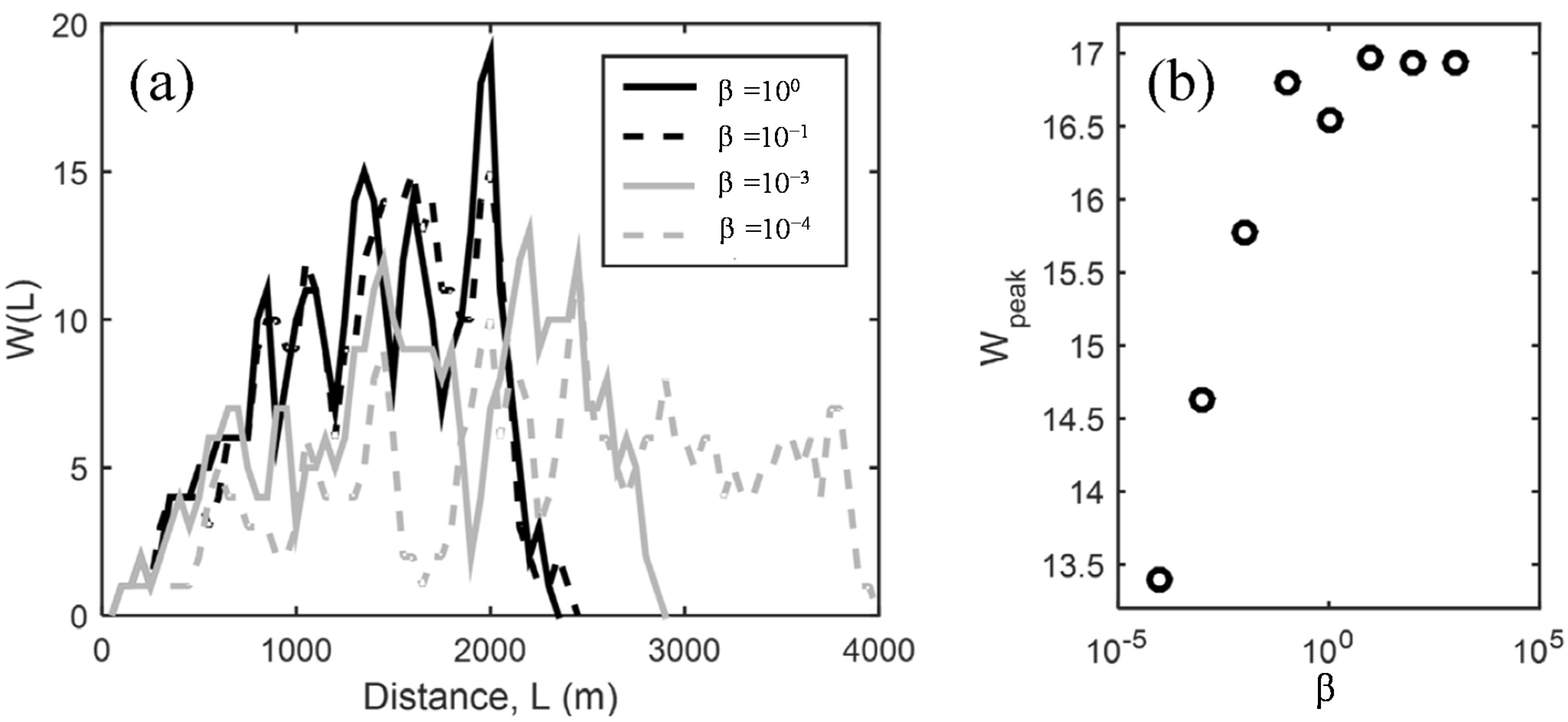
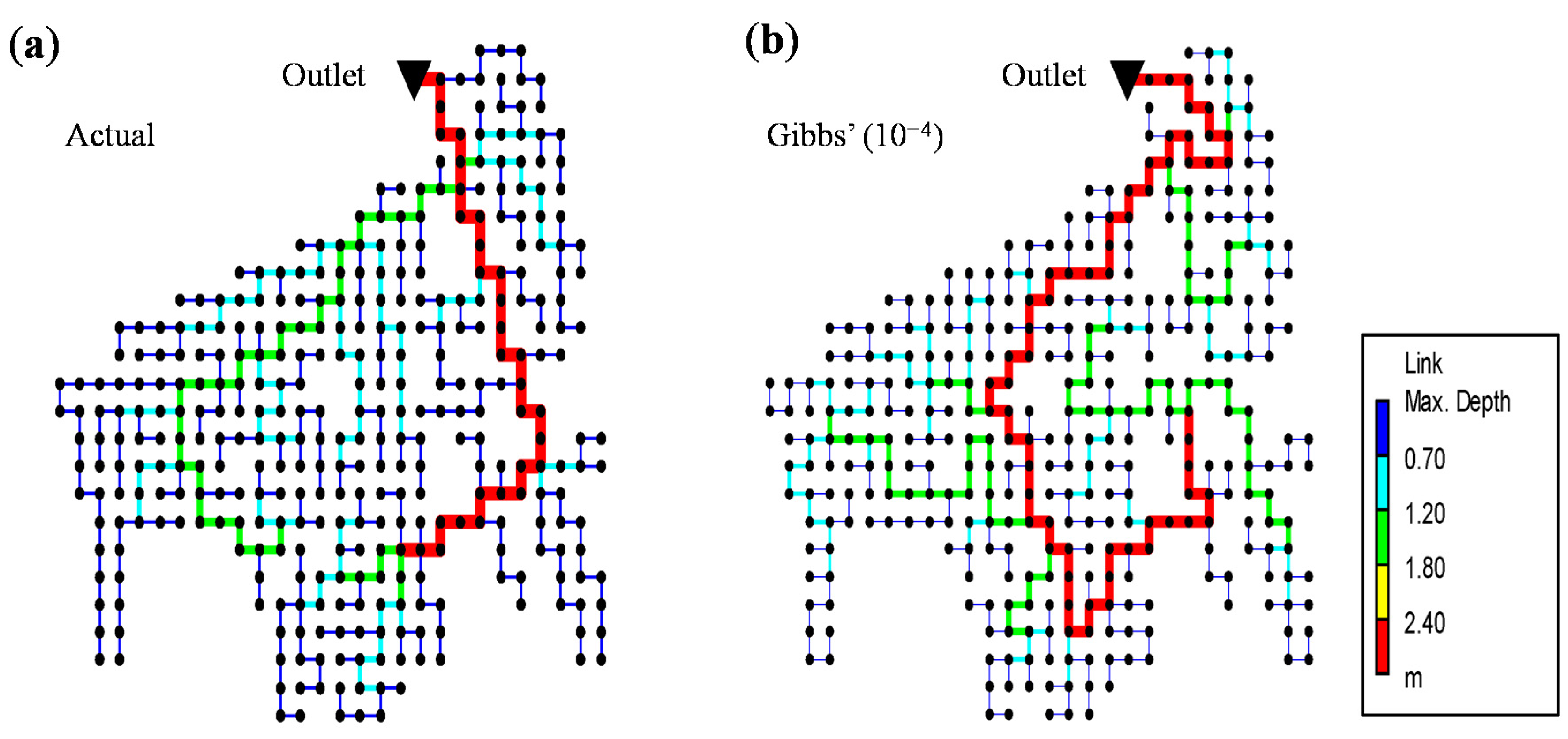
3.2. The Effect of Drainage Network Layout

| Order | Diameter (m) | Sp (%) | Length (m, Averaged) |
|---|---|---|---|
| 1 | 0.58 | 2.72 | 37.88 |
| 2 | 0.80 | 0.19 | 31.37 |
| 3 | 1.05 | 2.97 | 30.03 |
| 4 | 2.11 | 1.02 | 40.09 |
| 5 | 2.95 | 0.35 | 31.18 |


4. Conclusions
Acknowledgments
Author Contributions
Conflicts of Interest
References
- Choi, S.; Kang, S.; Han, S.; Lee, D.R. Urban flooding due to heavy rainstorm with focuses on gangnam areas in Seoul. Mag. Korea Water Resour. Assoc. 2011, 44, 25–29. [Google Scholar]
- Noh, S.J.; Tachikawa, Y.; Shiiba, M.; Kim, S. Ensemble Kalman filtering and particle filtering in a lag-time window for short-term streamflow forecasting with a distributed hydrologic model. J. Hydrol. Eng. 2013, 18, 1684–1696. [Google Scholar] [CrossRef]
- Brodie, I.M. Rational Monte Carlo method for flood frequency analysis in urban catchments. J. Hydrol. 2013, 486, 306–314. [Google Scholar] [CrossRef]
- Chang, F.J.; Chen, P.A.; Lu, Y.R.; Huang, E.; Chang, K.Y. Real-time multi-step-ahead water level forecasting by recurrent neural networks for urban flood control. J. Hydrol. 2014, 517, 836–846. [Google Scholar] [CrossRef]
- Chen, A.S.; Evans, B.; Djordjevic, S.; Savic, D.A. A coarse-grid approach to representing building blockage effects in 2D urban flood modelling. J. Hydrol. 2012, 426, 1–16. [Google Scholar] [CrossRef] [Green Version]
- Djordjević, S.; Prodanović, D.; Maksimović, Č. An approach to simulation of dual drainage. Water Sci. Technol. 1999, 39, 95–103. [Google Scholar] [CrossRef]
- Smith, M.B. A gis-based distributed parameter hydrologic model for urban areas. Hydrol. Process. 1993, 7, 45–61. [Google Scholar] [CrossRef]
- Zhang, S.H.; Wang, T.W.; Zhao, B.H. Calculation and visualization of flood inundation based on a topographic triangle network. J. Hydrol. 2014, 509, 406–415. [Google Scholar] [CrossRef]
- Rodriguez-Iturbe, I.; Valdes, J.B. Geomorphologic structure of hydrologic response. Water Resour. Res. 1979, 15, 1409–1420. [Google Scholar] [CrossRef]
- Saco, P.M.; Kumar, P. Kinematic dispersion in stream networks 1. Coupling hydraulic and network geometry. Water Resour. Res. 2002, 38, 1–14. [Google Scholar] [CrossRef]
- Haghighi, A. Loop-by-loop cutting algorithm to generate layouts for urban drainage systems. J. Water Resour. Plan. Manag. 2013, 139, 693–703. [Google Scholar] [CrossRef]
- Seo, Y.; Schmidt, A.R. The effect of rainstorm movement on urban drainage network runoff hydrographs. Hydrol. Process 2012, 26, 3830–3841. [Google Scholar] [CrossRef]
- Seo, Y.; Schmidt, A.R. Application of Gibbs’ model to urban drainage networks: A case study in southwestern Chicago, USA. Hydrol. Process 2014, 28, 1148–1158. [Google Scholar] [CrossRef]
- Troutman, B.M.; Karlinger, M.R. Gibbs distribution on drainage networks. Water Resour. Res. 1992, 28, 563–577. [Google Scholar] [CrossRef]
- Leopold, L.B.; Langbein, W.B. The Concept of Entropy in Landscape Evolution; U.S. Government Printing: Washington, DC, USA, 1962. [Google Scholar]
- Karlinger, M.R.; Troutman, B.M. A random spatial network model based on elementary postulates. Water Resour. Res. 1989, 25, 793–798. [Google Scholar] [CrossRef]
- Scheidegger, A.E. A stochastic model for drainage patterns into an intramontane trench. Int. Assoc. Sci. Hydrol. Bull. 1967, 12, 15–20. [Google Scholar] [CrossRef]
- Ising, E. Beitrag zur theorie des ferromagnetismus. Z. für Phys. A Hadron. Nucl. 1925, 31, 253–258. (In German) [Google Scholar] [CrossRef]
- Kindermann, R.; Snell, J.L. Markov Random Fields and Their Applications; American Mathematical Society: Ann Arbor, MN, USA, 1980. [Google Scholar]
- Seo, Y.; Schmidt, A.R. Network configuration and hydrograph sensitivity to storm kinematics. Water Resour. Res. 2013, 49, 1812–1827. [Google Scholar] [CrossRef]
- Seo, Y.; Schmidt, A.R. Evaluation of drainage networks under moving storms utilizing the equivalent stationary storms. Nat. Hazard. 2014, 70, 803–819. [Google Scholar] [CrossRef]
- Moussa, R. What controls the width function shape, and can it be used for channel network comparison and regionalization? Water Resour. Res. 2008, 44, 1–19. [Google Scholar] [CrossRef]
- Lashermes, B.; Foufoula-Georgiou, E. Area and width functions of river networks: New results on multifractal properties. Water Resour. Res. 2007, 43. [Google Scholar] [CrossRef]
- Lee, M.T.; Delleur, J.W. A variable source area model of the rainfall-runoff process based on the watershed stream network. Water Resour. Res. 1976, 12, 1029–1036. [Google Scholar] [CrossRef]
- Milly, P.C.D.; Betancourt, J.; Falkenmark, M.; Hirsch, R.M.; Kundzewicz, Z.W.; Lettenmaier, D.P.; Stouffer, R.J. Stationarity is dead: Whither water management? Science 2008, 319, 573–574. [Google Scholar] [CrossRef] [PubMed]
- Pachauri, R.K.; Reisinger, A. Contribution of Working Groups I, II and III to the Fourth Assessment Report of the Intergovernmental Panel on Climate Change; Intergovernmental Panel on Climate Change(IPCC): Geneva, Switzerland, 2007; p. 104. [Google Scholar]
- Huong, H.T.L.; Pathirana, A. Urbanization and climate change impacts on future urban flooding in Can Tho city, Vietnam. Hydrol. Earth Syst. Sci. 2013, 17, 379–394. [Google Scholar] [CrossRef]
- Seo, Y.; Schmidt, A.R.; Kang, B. Multifractal properties of the peak flow distribution on stochastic drainage networks. Stoch. Env. Res. Risk A 2014, 28, 1157–1165. [Google Scholar] [CrossRef]
- Mays, L.W. Water Resources Engineering; John Wiley: Hoboken, NJ, USA, 2011. [Google Scholar]
© 2015 by the authors; licensee MDPI, Basel, Switzerland. This article is an open access article distributed under the terms and conditions of the Creative Commons Attribution license (http://creativecommons.org/licenses/by/4.0/).
Share and Cite
Seo, Y.; Hwang, J.; Noh, S.J. Analysis of Urban Drainage Networks Using Gibbs’ Model: A Case Study in Seoul, South Korea. Water 2015, 7, 4129-4143. https://doi.org/10.3390/w7084129
Seo Y, Hwang J, Noh SJ. Analysis of Urban Drainage Networks Using Gibbs’ Model: A Case Study in Seoul, South Korea. Water. 2015; 7(8):4129-4143. https://doi.org/10.3390/w7084129
Chicago/Turabian StyleSeo, Yongwon, Junshik Hwang, and Seong Jin Noh. 2015. "Analysis of Urban Drainage Networks Using Gibbs’ Model: A Case Study in Seoul, South Korea" Water 7, no. 8: 4129-4143. https://doi.org/10.3390/w7084129