Predicting Dynamic Response of Structures under Earthquake Loads Using Logical Analysis of Data

Abstract

In this paper, logical analysis of data (LAD) is used to predict the seismic response of building structures employing the captured dynamic responses. In order to prepare the data, computational simulations using a single degree of freedom (SDOF) building model under different ground motion records are carried out. The selected excitation records are real and of different peak ground accelerations (PGA). The sensitivity of the seismic response in terms of displacements of floors to the variation in earthquake characteristics, such as soil class, characteristic period, and time step of records, peak ground displacement, and peak ground velocity, have also been considered. The dynamic equation of motion describing the building model and the applied earthquake load are presented and solved incrementally using the Runge-Kutta method. LAD then finds the characteristic patterns which lead to forecast the seismic response of building structures. The accuracy of LAD is compared to that of an artificial neural network (ANN), since the latter is the most known machine learning technique. Based on the conducted study, the proposed LAD model has been proven to be an efficient technique to learn, simulate, and blindly predict the dynamic response behaviour of building structures subjected to earthquake loads.

1. Introduction

It is a crucial issue to evaluate the response of building structures subjected to dynamic earthquake loads where seismic design of such buildings is generally carried out on the basis of the results obtained from the performed dynamic analysis. Seismic response evaluation of building structures mainly involves determination and assessment of displacement demands [1,2,3]. Characteristics of ground excitations having various peak ground accelerations, together with the dynamic properties of structures, are potentially the most important factors affecting the seismic response behaviour. The accurate prediction of the dynamic response of structures subjected to ground motions from possible future earthquakes can be considered as the first step towards introducing possible mitigation techniques and preventing structural damage against sudden earthquake hazards. The most suitable method for assessing the response of building structures is nonlinear dynamic analysis. Based on the results obtained from the analysis, conclusions regarding the design capacity, as well as the ductility requirements for each structural element or of the whole structural systems, can be obtained [4]. Ductility is considered as the main factor controlling the damage of structures, as well as an indication of seismic vulnerability of newly-designed or existing under-designed buildings [5]. The vulnerability of building structures under earthquake records of known characteristics can be defined as the degree of damage to a structure [6].

The seismic response of building structures using artificial intelligence techniques has captured the interest of many researchers who studied the issues concerning the applications of artificial intelligence techniques to engineering structures. Parsaei Maram et al. [7] performed an investigation to predict the seismic behaviour of reinforced concrete buildings with and without infill walls using an artificial neural network. Pei and Smyth [8] introduced a new architecture of a multilayer feedforward neural network for problems with nonlinear and hysteric dynamic behaviours of single-degree-of-freedom oscillators. Several attempts were also undertaken to investigate the importance of considering the neural networks on a prestressed concrete bridge subjected to earthquake excitation [9]. However, most of the studies on earthquake-induced structural response have been conducted using artificial intelligence techniques. To date, the logical analysis of data (LAD) has not been devoted yet to study the response behaviour of buildings.

This paper uses the machine learning technique LAD to predict seismic response of building structures. A MATLAB (Matrix Laboratory) code has been developed to serve for simulating the dynamic response of the SDOF building system. For the purpose of generating input data for the LAD model, 200 observations from exciting the SDOF building model are collected. A suite of 20 ground motion records from different regions and with different characteristics are used in the dynamic time-history analysis of the SDOF model having different natural periods. The natural period of the considered building model ranges from 0.1 s to 1 s. In Section 2, the building model and data preparation are presented. In Section 3, System parameters and input ground motion are introduced. In Section 4 and Section 5, the training process, from the experimental data, is introduced and comparison between LAD and the well-known ANN technique is presented. Then, results and discussion are presented. The validation process is presented in Section 7, and concluding remarks are given in the last section.

2. Building Model

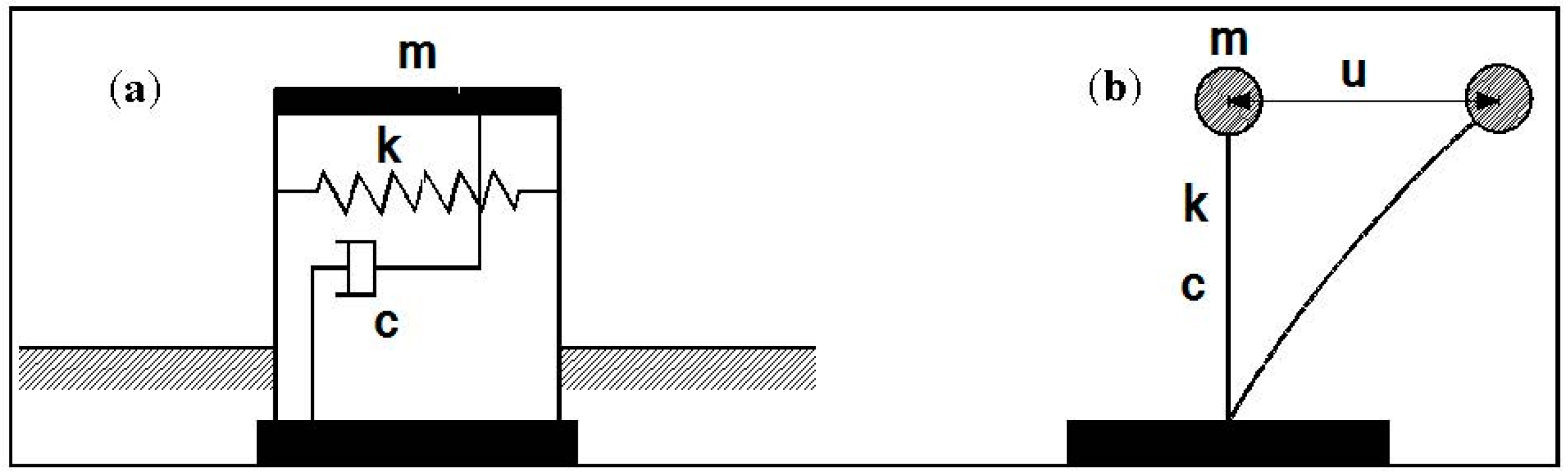
Consider the structural building model and its idealized single degree of freedom mathematical model as shown in Figure 1. The symbol m represents the mass of the superstructure of the building model. The structural damping and stiffness coefficients of the building are represented by c and k, respectively. The values of structural stiffness and damping coefficients can be calculated from the following formulas [10]:

$$k=\frac{4{\pi }^{2}m}{T^2};C=2\xi \sqrt{km}$$

(1)

where T and ξ denote the natural structural vibration period and structural damping, respectively.

The governing equation of motion for the structural building system shown in Figure 1 can be written as follows:

$$m\ddot{u}\left(t\right)+c\dot{u}\left(t\right)+ku\left(t\right)=-m{\ddot{u}}_g\left(t\right)$$

(2)

The derivatives with respect to time in terms of $\ddot{u}$ and $\dot{u}$ respectively represent the relative acceleration and relative velocity of superstructure. $u$ represents the relative displacement of the building model superstructure. The earthquake ground acceleration is denoted by ${\ddot{u}}_g$. Response analysis of building structures under random dynamic forces, such as earthquake, wind, and blast loads, requires the use of an efficient numerical integration technique where the accuracy of the employed technique is of great importance for practical design. The dynamic solution to the second-order ordinary differential equations in Equation (2) is performed using the Runge-Kutta (RK) methods. The ordinary differential equation in Equation (2) is equivalent to the following first-order system [11]:

$$\begin{array}{c}\dot{u}\left(t\right)=v\left(t\right)\\ \dot{v}\left(t\right)=-\frac{c}{m}v\left(t\right)-\frac{k}{m}u\left(t\right)-{\ddot{u}}_g\left(t\right)\end{array}$$

(3)

Assuming:

$$U=\left(\begin{array}{c}u\left(t\right)\\ v\left(t\right)\end{array}\right)$$

(4)

$$f\left(t\right)=\left(\begin{array}{c}v\left(t\right)\\ -\frac{c}{m}v\left(t\right)-\frac{k}{m}u\left(t\right)-{\ddot{u}}_g\left(t\right)\end{array}\right)$$

(5)

Equations (4) and (5), together with the initial condition U(0) = 0, provide the following system of autonomous ordinary first-order differential equation:

$$\frac{dU}{dt}=f\left(t\right),U\left(0\right)=U_0$$

(6)

A MATLAB code based on the explicit fourth-order RK method of has been developed in order to obtain the numerical solution of Equation (6), which is equivalent to the second-order ordinary differential equation in Equation (2). In order to ensure reasonable accuracy with a quick solution to the above system using the fourth-order Runge-Kutta method, the chosen step size Δt over the time interval has to be of a value less than one-tenth of the building’s natural period [12].

3. System Parameters and Input Ground Motion

This section defines the parameters of the considered building model, as well as the set of ground motions used to excite the building model. Details of the aforementioned information are provided in the following two subsections.

3.1. System Parameters

The dynamic parameters of the building structure considered in the current study are taken from an earlier study by Jankowski [13].

Table 1. The dynamic parameters of the used building structure.

Mass (m)	25 × 103 kg
Damping ratio (ξ)	0.05
Initial stiffness (k)	3.46 × 106 N/m

shows the basic values describing the structural characteristics used in the analysis.

3.2. Input Ground Motion

A set of 20 earthquake ground motion records from different regions and different peak ground accelerations (see

Table 2. Strong ground motion records used as the input to adjacent buildings.

Earthquake (Record)	PGA (g)	PGV (cm/s)	PGD (cm)	Mw	EPD (km)	Soil Class	Tg (s)
Imperial Valley	0.1	8.2	1.4	5.2	15.6	D, C	0.75
San Fernando	0.1	6.4	1.4	6.6	25.7	D, B	0.85
Northridge	0.11	8.7	1.8	6.7	22.7	A, A	0.8
Loma Prieta	0.19	12.7	5.5	6.9	43.4	B, NA	0.7
Morgan Hill	0.19	11.2	2.4	6.2	14.6	D, C	1.1
Palm Springs	0.21	40.9	15	6	10.1	C, B	1.9
Morgan Hill	0.29	36.7	6.1	6.2	11.8	B, B	1.2
Loma Prieta	0.37	27.2	3.8	6.9	16.9	D, NA	0.85
Northridge	0.48	62.8	11.1	6.7	19.6	C, B	0.85
Loma Prieta	0.48	39.7	15.2	6.9	21.8	A, NA	0.65
Northridge	0.49	45.1	12.6	6.7	12.1	D, C	0.7
Northridge	0.51	52.2	2.4	6.7	22.6	B, B	0.95
Cape Mendocino	0.59	48.4	21.7	7.1	9.5	D, C	0.75
Palm Springs	0.59	73.3	11.5	6	8.2	D, B	1.1
Coalinga	0.6	34.8	8.1	5.8	17.4	D, NA	0.65
Loma Prieta	0.61	51	11.5	6.9	6.1	A, NA	0.8
Duzce	0.82	62.1	13.9	7.1	17.6	D, C	0.9
Coalinga	0.84	44.1	6.8	5.8	9.2	A, NA	0.75
Chi-Chi	0.9	102.4	34	7.6	6.8	C, C	1
Cape Mendocino	1.04	42	12.4	7.1	8.5	A, A	2

) is used in the current research study as inputs to excite the building model shown in Figure 1. These selected records are from 1971 Imperial Valley (El Centro), 1994 Northridge, 1971 San Fernando, 1989 Loma Prieta, 1984 Morgan Hill, 1986 Palm Springs, 1992 Cape Mendocino, 1983 Coalinga, 1999 Duzce, and 1999 Chi-Chi earthquakes. Important information related to the selected earthquake records, such as earthquake peak ground acceleration (PGA), peak ground velocity (PGV), peak ground displacement (PGD), magnitude (Mw), site to source distance (EPD), soil class (USGS), and characteristic period (Tg), can be found in Table 2. These selected earthquake records represent various ground motion records with different PGA that varies between 0.1 g and 1.04 g, where g is the acceleration of gravity, in order to ensure low (0.1–0.4), moderate (0.4–0.7), and high (0.8–1.2) PGA levels during the numerical simulations. Different frequency contents, total durations, and local soil conditions are also characteristics of the selected ground motions. The magnitude of the chosen earthquake records varies between 5.2 and 7.1 with site-source distances of about 6.1 km to 43.3 km, which implies that the selected ground motions contain far-fault, as well as near-fault, motions. It is worth noting that the moment magnitude of moderate, strong, major, and great earthquakes vary between 5 to 5.9, 6 to 6.9, 7 to 7.9, and 8 to 8.9, respectively.

4. Logical Analysis of Data (LAD)

LAD is a method for data analysis using concepts from supervised machine learning, combinatorics, and Boolean functions which is conceded as a knowledge discovery technique first developed in 1986 [14,15]. The methodology of LAD consists of three steps: binarization of data, pattern generation, and theory formation. For more details about data binarization see [16]. Many techniques for pattern generation are adopted by many researchers, such as enumeration [16], heuristics [14,17], and integer linear programming [18]. This last one has been proposed in this paper. In the last step, the discriminant function $\Delta \left(\mathrm{O}\right)$ is used as follows [19]:

$$\Delta \left(\mathrm{O}\right)=\underset{m=1,\dots ,Z}{argmax}{S}_m\left(\mathrm{O}\right)$$

(7)

where $S_m\left(\mathrm{O}\right)={\displaystyle \sum }_{P_n\in {\mu }_m}{\alpha }_n{P}_n\left(\mathrm{O}\right)$, $P_n$ is the corresponding pattern in set ${\mathsf{\mu }}_{\mathrm{m}}$ covering observation O, and ${\alpha }_n>0$ is the coverage rate of pattern $P_n\in {\mu }_m\left(m=1,\dots ,Z\right)$ with respect to the observations of the class. Pattern $P_n\left(O\right)=1$ if it covers observation $\mathrm{O}$, and zero otherwise.

The accuracy ($AC$) of classification is:

$$AC=\frac{{{\displaystyle \sum }}_m^z{G}_m}{Nt},$$

(8)

where $G_m$ is the number of correctly-classified observations in class $m$, and $Nt$ is the number of observations in the testing set.

5. Artificial Neural Network (ANN)

The artificial neural network is the most famous and well-known machine learning technique. An ANN is composed of three types of layers, namely, an input layer, hidden layer(s), and an output layer. The input layer is responsible for accepting input attributes so as to be equal to the number of neurons. In the hidden layer, some number of neurons are contained. On the other hand, the output layer is only a single neuron. It is worth noting that the nonlinearity of the model highly influences the number of hidden layers and the contained neurons. The contained neurons in any of the aforementioned layers are directly related through weighted links to the neurons of pre- and post-layers. Each neurons of the hidden and output layers is offset by a threshold value. It has high efficiency on adaptation and learning.

The accuracy of LAD is compared with that of an ANN, since the latter is the best-known machine learning technique.

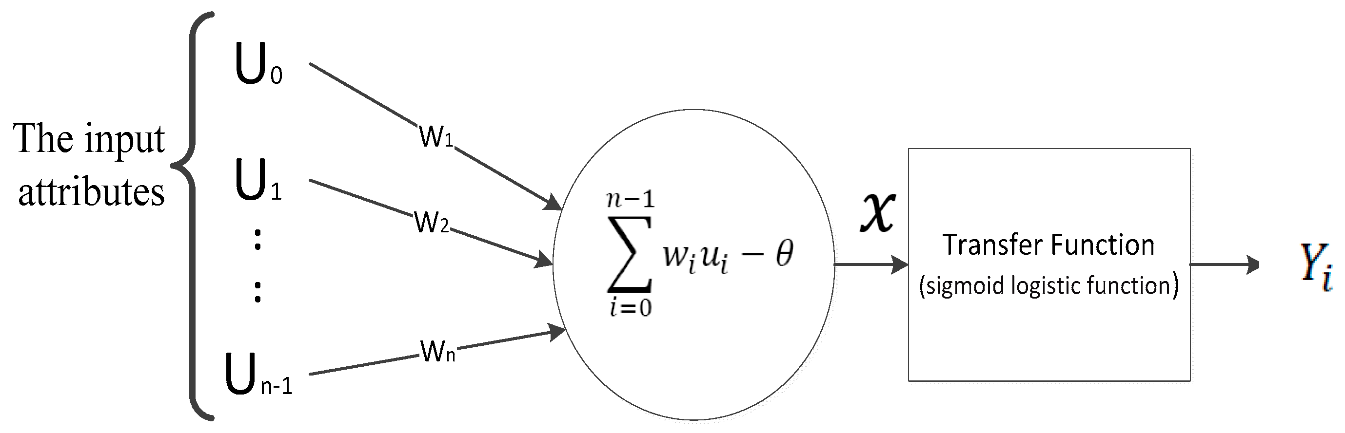
The mathematical model of an artificial neuron’s behaviour imitates a mathematical model of a brain’s activity [20]. Figure 2 shows the behaviour of an artificial neuron .The input attributes $u\left(n\right)$ to the network weighted by $w\left(n\right)$ are sent to a neuron. By performing accumulation, the neuron sums the weighted inputs, passes the result to a transfer function, and provides an output $Y_i$ [21]:

$$Y_i=f\left({\displaystyle \sum }_{i=0}^{n-1}{w}_i{u}_i-\theta \right)$$

(9)

where $\theta \in \left(-\infty ,\infty \right)$ is the internal threshold; the inputs $u\left(n\right)$ in this work are the input attributes, either controllable or uncontrollable (monitoring), as we will see later in Section 5; and $f$ is the non-linear transfer function. The most commonly-used $f$ is defined by the sigmoid logistic function as:

$$f\left(x\right)=\frac{1}{1+e^{-x}}$$

(10)

The output of the sigmoid function is always between [0,1] which can be used to classify the quality outcome to conforming the specification and nonconforming. In other words, the sigmoid function squashes any value of $\mathrm{x}$ to specify the probability of the binary output $y_i=\in \left\{0,1\right\}$ given the input $u_i$. Back-propagation (BP) is used to update the weights $w_i$ dynamically.

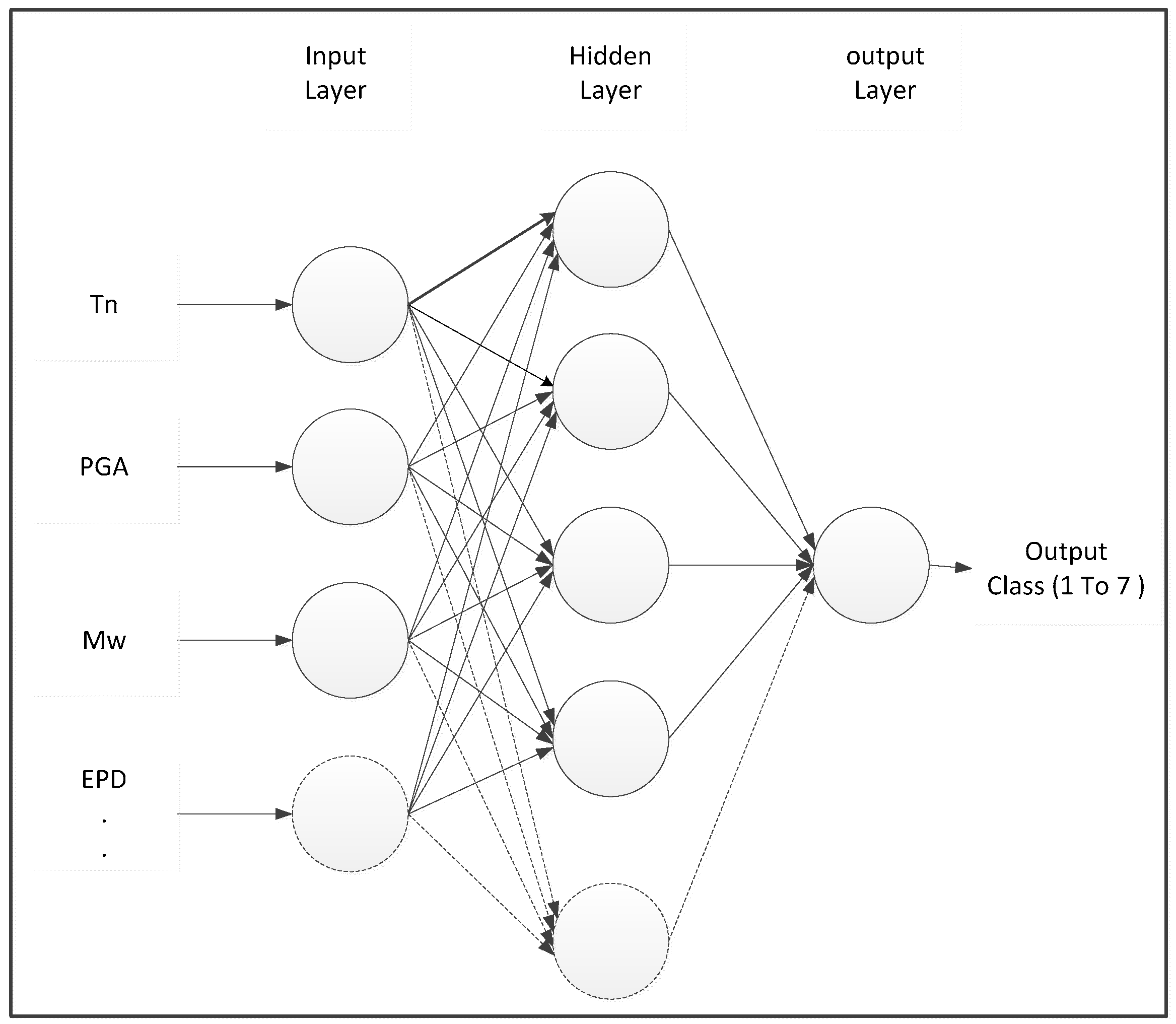
An ANN consists of three types of layers, namely, an input layer, hidden layer(s), and an output layer. In Figure 3, the input layer accepts the inputs, which are the eight variables; seven variables describe the earthquakes and one variable describes the building. The seven variables are peak ground acceleration, peak ground velocity, peak ground displacement, soil class, characteristic period, magnitude, and site-source distance, and the one variable that describes the building is the natural period.

6. Results and Discussion

The collected data is used to train LAD to determine the displacement class by finding hidden patterns that are specific to each class. The found patterns are represented in terms of the variables which describe the used earthquakes and the building. Each pattern is a special rule that is hidden in the data, and which is specific to a certain class. The input data are the 200 observations selected from the simulation analysis using the considered earthquake records. Seven classes of seismic response have been used in the analysis. Each observation contains the measurement of eight covariances and one of the seven labels. The covariances are: peak ground acceleration, peak ground velocity, peak ground displacement, soil type, characteristic period, magnitude, site-source distance, and the natural period. Seismic response is classified into seven classes, as shown in

Table 3. Seven classes’ ranges and their number of observations.

Class	Range		Number of Observation
	To (mm)	From (mm)
D1	15	0	67
D2	30	15.1	32
D3	60	30.1	32
D4	100	60.1	24
D5	150	100.1	18
D6	200	150.1	18
D7	>201.1	200.1	9

.

The building model presented in Figure 1 has been subjected to a set of 20 earthquake excitation records. The used earthquake characteristics in terms of PGA, PGV, PGD, magnitude, epicentre distance, soil class, and characteristic period are listed in Table 1. Several natural periods varying from 0.1s to 1 s have been assigned to the considered building model. In

Table 4. A sample of the results that represent the first six readings from the analysis.

No	Tn	PGA	Mw	EPD	PGV	PGD	Soil	Tg	Class
1	0.1	0.1	1	15.6	8.2	1.4	3	0.75	D1
2	0.1	0.1	2	25.7	6.4	1.4	2	0.85	D1
3	0.1	0.11	2	22.7	8.7	1.8	1	0.8	D1
4	0.1	0.19	2	43.4	12.7	5.5	2	0.7	D1
5	0.1	0.19	2	14.6	11.2	2.4	3	1.1	D1
6	0.1	0.21	2	10.1	40.9	15	2	1.9	D1

, the moment magnitude of earthquake is considered moderate from 5 to 5.9 and labelled (1); strong from 6 to 6.9 and labelled (2); major from 7 to 7.9 and labelled (3) and; finally, great from 8 to 8.9 and labelled (4). The total number of results produced from the simulation analysis are about 200 (20 results for each natural period under the list of records in Table 1). The obtained results have been classified into seven categories. Table 4 exhibits the patterns found by the software cbmLAD [22] and shows the first six observation out of 200 as an example of the collected data.

The sensitivity of the seismic response of the building model with several natural periods to the characteristics of the considered earthquake records in terms of PGA, PGV, PGD, magnitude of the earthquake, site-source distance, soil class, and characteristic period, Tg, have also been tabulated in

Table 5. Patterns found by the software cbmLAD.

Lass	Pattern	Tn	PGA	Mw	EPD	PGV	PGD	Soil	Tg
1	1	<0.25	-	-	-	-	-	-	-
	2	<0.45	<0.25	-	-	-	-	-	-
	3	<0.55	<0.45	-	-	-	<3.1	-	-
	4	<0.65	<0.25	-	-	<11.95	<2.1	-	-
	5	-	<0.25	-	>24.2	<11.95	-	-	-
	6	>0.55, <0.95	<0.33	-	>24.2	<31	-	-	-
2	1	>0.25, <0.35	>0.25	-	>10.95, <24.2	-	>2.1	-	-
	2	>0.25, <0.35	>0.25	>2.5	-	-	-	-	-
	3	>0.25, <0.35	>0.595	-	-	-	-	-	-
	4	>0.25, <0.45	>0.25	-	-	-	<6.45	-	-
	5	>0.25, <0.45	>0.5	-	<8.85	-	>12.5	-	-
	6	>0.45, <0.55	-	-	<34.55	-	-	-	-
	7	>0.45, <0.55	<0.45	-	-	-	>14.45	-	>0.875
	8	>0.55, <0.85	-	-	-	<11.95	-	-	>0.975
	9	>0.25, <0.65	-	-	-	-	-	>3.5	-
	10	>0.65	-	<1.5	-	<11.95	-	-	-
	11	>0.65, <0.95	-	-	-	-	<3.1	-	<0.825
	12	>0.95,	-	-	>34.55	-	-	-	-
3	1	>0.25, 0.55	>0.55, <0.605	-	>6.45, <8.35	-	>5.8	-	-
	2	>0.35, <0.45	>0.33	-	-	-	>6.45	-	<0.925
	3	>0.35, <0.55	>0.45	-	>7.5, <17.5	>19.95	>7.45	-	-
	4	>0.45, <0.55	>0.25	-	-	-	-	-	>0.925
	5	>0.35, <0.55	-	-	-	-	-	-	<0.675
	6	>0.55, <0.65	-	-	-	-	-	-	>1.55
	7	>0.45, <0.65	>0.25	-	<12	<43.05	-	-	>0.925
	8	>0.65, <0.75	-	-	<12	-	>11.95	-	>1.05
	9	>0.65, <0.75	-	-	-	-	-	>3.5	-
	10	>0.75	-	<1.5	-	-	-	-	<0.675
	11	>0.85	-	-	-	<11.95	-	-	>1.05
	12	>0.95	-	-	>22.65	-	-	<1.5	-
4	1	>0.45, <0.75	>0.25	-	>17.15	>40.3	>6.45	<2.5	-
	2	>0.45, <0.65	>0.25	-	-	>49.7	>6.45	<1.5	-
	3	>0.45, <0.55	>0.605	-	>17.5	-	-	-	-
	4	>0.45, <0.55	>0.605	<1.5	-	-	-	-	-
	5	>0.55, <0.75	-	-	<17.5	>31	-	-	<0.725
	6	>0.55, <0.65	-	-	>22.2	>49.7	-	-	-
	7	>0.55, <0.75	>0.395	-	-	>62.45	-	-	>1.05
	8	>0.55, <0.65	-	-	<8.85	>49.7	-	-	-
	9	>0.65, <0.75	-	-	-	<38.2	-	-	>1.15
	10	>0.75	-	-	-	-	-	-	>1.55
	11	>0.75, <0.85	>0.33, <0.485	-	-	<44.6	-	-	-
	12	>0.75	>0.33,	-	-	>31, <43.05	>11.3	<2.5	-
5	1	>0.55, <0.75	>0.45	-	-	>35.75, <62.45	>15.1	<2.5	-
	2	>0.55, <0.65	-	-	-	-	>13.25	-	<0.925
	3	>0.55, <0.65	-	-	<9.8	>43.05	-	-	<0.775
	4	>0.65, <0.75	>0.25	-	-	>49.7	<6.45	-	>0.925
	5	>0.65, <0.75	-	-	<7.5	-	-	-	-
	6	>0.75, <0.85	-	-	-	>35.75	<11.95	-	>0.925
	7	>0.85	>0.25	-	-	<38.2	<7.45	-	-
	8	>0.95	-	-	<6.45	-	-	-	-
6	1	>0.65	>0.5	-	<20.7	>43.05	-	-	<0.775
	2	>0.65, <0.75	>0.715	-	-	-	-	-	-
	3	>0.75, <0.85	-	-	-	>43.05	-	-	<0.875
	4	>0.75, <0.85	-	-	<7.5	>43.05	-	-	-
	5	>0.75, <0.95	-	-	<13.4	>43.05	>6.45	-	<0.975
	6	>0.85	>0.485	-	>22.2	>43.05	-	-	-
	7	>0.85, <0.95	>0.5	-	-	>43.05	<11.95	-	-
7	1	>0.75	-	-	>17.5	>57.15	>11.3	-	<1.05
	2	>0.85	-	-	-	>57.15	-	-	<1.05
	3	>0.95	-	-	-	>44.6	>9.6, <14.45	>1.5	-

. The software cbmLAD has been employed to find the aforementioned tabulated results. The obtained results clearly indicate that the fundamental natural period, Tn, one of the most important parameters that affects the building model seismic response, appears in all the grouped classes of results. The epicentre distance has also been found to highly affect the simulation response results. On the contrary, the moment magnitude Mw of the earthquake has been found to be slightly affect the induced seismic responses. This can be due to Mw being considered as a measure of the amount of earthquake energy released and a measure of damage as well. Similarly, the USCS, which is a unified soil classification system used to describe the texture and grain size of a soil, slightly affects the seismic response results. It is worth noting that the characteristic period, Tg, or in other words the dominant period of an earthquake, showed a pronounced effect on the response prediction of structures. The rigid structures are more affected by the waves with short Tg or high frequency. On the other hand, flexible structures, such as high-rise buildings, are more affected by long Tg (see classes 2–7). Destruction occurs when any of the natural frequencies of the building model coincide with the dominant frequency of the applied earthquake.

7. Validation and Comparison

The observed experimental values have been divided into two types of sets, namely, the learning set and testing set, like many machine learning techniques. The ten-fold cross-validation procedure used herein is performed by randomly dividing all of the observations into ten parts. The divided classes are approximately represented such as to have a similar proportion as in the full dataset. The first set, which is sometimes called the testing set T, is held out. This set represents about 10% of the total observations. The remaining 90% is associated to the trained set required for performing the learning process. The aforementioned percentage values clearly indicate that most of the observations are used for the training process, thus increasing the chance that the classifier found is an accurate one. The average accuracy ($A$) of learning is found to be equal to 0.84.

For the purpose of achieving the highest accuracy of prediction during the validation test, the architecture network is used [20]. In this paper, Weka data mining software [23] is used to enable obtaining the best network structure. Several trials are performed as a common approach to find the best architecture and then keep it as the recommended one [20].

Figure 4 shows the best architecture found by Weka. It has one hidden layer of four neurons, a learning rate of 0.2, and a momentum of 0.2. The same ten-fold cross-validation procedure is performed; the confusion matrix is shown in

Table 6. Confusion matrix for the grouped classes of results.

Class 1	Class 2	Class 3	Class 4	Class 5	Class 6	Class 7
62	5	0	0	0	0	0	Class 1
5	26	1	0	0	0	0	Class 2
1	5	22	4	0	0	0	Class 3
0	0	3	15	3	4	1	Class 4
0	0	1	5	10	0	0	Class 5
0	0	0	6	2	9	1	Class 6
0	0	0	1	3	1	4	Class 7

.

$G_m$ and $G_m^l$ respectively denote the number of correctly and incorrectly classified observations in class $\mathrm{m}$. The superscript 1 refers to class $\mathrm{l}$, $l$ ≠ $m$. For example, $G_1=62\mathrm{and}{G}_1^3=5$ refer to the number of correctly-classified observations in class 1, the number of incorrectly classified observations in class 1, and those classified as class 2. The learning accuracy ($\mathrm{AC}$) has been found to be:

$$AC=\frac{{{\displaystyle \sum }}_m^z{G}_m}{\mathrm{Nt}}=\frac{62+26+22+15+10+9+4}{200}=0.74$$

(11)

The LAD accuracy proved to be efficient as compared with that of the ANN. After finishing the training process and starting to analyse sensors to the test or new readings, which is not included in the original dataset, LAD has been found to be powerful in predicting the induced displacement response class based on the found patterns in each new observation. The new observation belongs to the class with the highest score regarding the value $\Delta \left(\mathrm{O}\right)$. In general, LAD has the advantages of the causality property, which makes it very useful in tackling engineering problems. This means that one can track back results, phenomena, or effects to their possible causes. This clearly recommends the use of LAD, especially when compared to ANN, in which the user may face some difficulties in determining the required number of nodes, as well as the network structure. Moreover, interpreting the classification process is an additional difficulty. This is “black box” procedure of the causality relationship which classifies new observations without any deep explanation.

8. Conclusions

The current research study presents an efficient and reliable technique based on the LAD process for predicting the seismic response behaviour of building structures under ground excitations using the captured dynamic responses. A SDOF building model with different natural periods has been subjected to a set of earthquake records with different characteristics. The LAD technique has been employed to capture the sensitivity of the seismic responses to the characteristics of the applied ground motions. From a building dynamic characteristics point of view, analysis of the obtained results clearly indicated that the variations in the building’s natural period significantly affect the captured dynamic responses. From the earthquake characteristics point of view, the epicentre distance has also been found to highly affect the obtained seismic response results. On the other hand, the moment magnitude, as one of the earthquake characteristics, has been found to slightly affect the induced seismic responses. Based on the conducted study, the proposed LAD model has been proven to be an efficient technique to learn, simulate, and blindly predict the dynamic response behaviour of building structures subjected to earthquake loads.

References

- Chopra, A.K.; Goel, R.K. A modal pushover analysis procedure to estimate seismic demands for buildings: Theory and preliminary evaluation. Civ. Environ. Eng. 2001, 55. [Google Scholar]
- Park, K.; Medina, R.A. Conceptual seismic design of regular frames based on the concept of uniform damage. J. Struct. Eng. 2007, 133, 945–955. [Google Scholar] [CrossRef]
- Villaverde, R. Methods to assess the seismic collapse capacity of building structures: State of the art. J. Struct. Eng. 2007, 133, 57–66. [Google Scholar] [CrossRef]
- Okada, S.; Takai, N. Classifications of structural types and damage patterns of buildings for earthquake field investigation. In Proceedings of the 12th World Conference on Earthquake Engineering, Auckland, New Zeland, 30 January–4 February 2000; p. 705. [Google Scholar]
- Abrams, D.P.; Calvi, G. Summary of the ATC-33 project on guidelines for seismic rehabilitation of buildings. In Technical Report; US National Center for Earthquake Engineering Research: Buffalo, NY, USA, 1994; pp. 11–23. [Google Scholar]
- Sun, L.; Yu, G.; Sun, Z. Bi-parameters method for structural vulnerability analysis. Intell. Autom. Soft Comput. 2010, 16, 747–754. [Google Scholar] [CrossRef]
- Maram, M.P.; Rao, K.R.M.; Poursalehi, A. Anartificial Neural Network for Prediction of Seismic Behavior in RC Buildings with and Without Infill Walls. Int. J. Mod. Eng. Res. 2013, 1, 3071–3078. [Google Scholar]
- Pei, J.-S.; Smyth, A.W. New approach to designing multilayer feedforward neural network architecture for modeling nonlinear restoring forces. II: Applications. J. Eng. Mech. 2006, 132, 1301–1312. [Google Scholar] [CrossRef]
- Jeng, C.-H.; Mo, Y. Quick seismic response estimation of prestressed concrete bridges using artificial neural networks. J. Comput. Civ. Eng. 2004, 18, 360–372. [Google Scholar] [CrossRef]
- Harris, C.M.; Piersol, A.G. Harris’ Shock and Vibration Handbook; McGraw-Hill: New York, NY, USA, 2002; Volume 5. [Google Scholar]
- Chen, X.; Mahmoud, S. Implicit Runge-Kutta methods for Lipschitz continuous ordinary differential equations. SIAM J. Numer. Anal. 2008, 46, 1266–1280. [Google Scholar] [CrossRef]
- Butcher, J.C. Numerical Methods for Ordinary Differential Equations; John Wiley & Sons: Hoboken, NJ, USA, 2008. [Google Scholar]
- Jankowski, R. Earthquake-induced pounding between equal height buildings with substantially different dynamic properties. Eng. Struct. 2008, 30, 2818–2829. [Google Scholar] [CrossRef]
- Hammer, P.L. Partially defined Boolean functions and cause-effect relationships. In Proceedings of the International Conference on Multi-Attribute Decision Making via or-Based Expert Systems, Passau, Germany, 20–27 April 1986. [Google Scholar]
- Crama, Y.; Hammer, P.L.; Ibaraki, T. Cause-effect relationships and partially defined Boolean functions. Ann. Oper. Res. 1988, 16, 299–325. [Google Scholar] [CrossRef]
- Bores, E.; Hammer, P.L.; Ibaraki, T.; Kogan, A.; Mayoraz, E.; Muchnik, I. An implementation of logical analysis of data. IEEE Trans. Knowl. Data Eng. 2000, 12, 292–306. [Google Scholar] [CrossRef]
- Hammer, P.L.; Bonates, T.O. Logical analysis of data—An overview: From combinatorial optimization to medical applications. Ann. Oper. Res. 2006, 148, 203–225. [Google Scholar] [CrossRef]
- Ryoo, H.S.; Jang, I.Y. Milp approach to pattern generation in logical analysis of data. Discret. Appl. Math. 2009, 157, 749–761. [Google Scholar] [CrossRef]
- Herrera, J.F.A.; Subasi, M.M. Logical Analysis of Multi Class Data; No. RRR 5-2013; Rutcor Research Report; Rutgers University: New Brunswick, NJ, USA, March 2013. [Google Scholar]
- Russell, S.J.; Norvig, P.; Canny, J.F.; Malik, J.M.; Edwards, D.D. Artificial Intelligence: A Modern Approach; Prentice Hall Englewood Cliffs: Upper Saddle River, NJ, USA, 1995; Volume 74. [Google Scholar]
- Zhang, J.Z.; Chen, J.C.; Kirby, E.D. The development of an in-process surface roughness adaptive control system in turning operations. J. Intell. Manuf. 2007, 18, 301–311. [Google Scholar] [CrossRef]
- Yacout, S.; Salamanca, D.; Mortada, M.-A. Tool and Method for Fault Detection of Devices by Condition Based maintenance. WO Application Wo 2012/009804A1, 26 January 2012. [Google Scholar]
- Hall, M.; Frank, E.; Holmes, G.; Pfahringer, B.; Reutemann, P.; Witten, I.H. The WEKA data mining software: An update. ACM SIGKDD Explor. Newsl. 2009, 11, 10–18. [Google Scholar] [CrossRef]
Figure 1.
(a) Structural building model; and (b) the idealized SDOF mathematical model.
Figure 2.
The behaviour of an artificial neuron.
Figure 3.
ANN models.
Figure 4.
ANN architecture.