How Much Do Clouds Mask the Impacts of Arctic Sea Ice and Snow Cover Variations? Different Perspectives from Observations and Reanalyses


Department of Atmospheric and Oceanic Sciences, University of Wisconsin-Madison, 1225 West Dayton St., Madison, WI 537111, USA
*
Author to whom correspondence should be addressed.
Atmosphere 2019, 10(1), 12; https://doi.org/10.3390/atmos10010012
Submission received: 16 October 2018
/
Revised: 21 December 2018
/
Accepted: 1 January 2019
/
Published: 4 January 2019
(This article belongs to the Special Issue Atmospheric Processes Shaping Arctic Climate)
Abstract
:Decreasing sea ice and snow cover are reducing the surface albedo and changing the Arctic surface energy balance. How these surface albedo changes influence the planetary albedo is a more complex question, though, that depends critically on the modulating effects of the intervening atmosphere. To answer this question, we partition the observed top of atmosphere (TOA) albedo into contributions from the surface and atmosphere, the latter being heavily dependent on clouds. While the surface albedo predictably declines with lower sea ice and snow cover, the TOA albedo decreases approximately half as much. This weaker response can be directly attributed to the fact that the atmosphere contributes more than 70% of the TOA albedo in the annual mean and is less dependent on surface cover. The surface accounts for a maximum of 30% of the TOA albedo in spring and less than 10% by the end of summer. Reanalyses (ASR versions 1 and 2, ERA-Interim, MERRA-2, and NCEP R2) represent the annual means of surface albedo fairly well, but biases are found in magnitudes of the TOA albedo and its contributions, likely due to their representations of clouds. Reanalyses show a wide range of TOA albedo sensitivity to changing sea ice concentration, 0.04–0.18 in September, compared to 0.11 in observations.
1. Introduction
Since the beginning of the satellite era, sea ice in the Northern Hemisphere (NH) has decreased in September extent, thinned substantially, and undergone earlier and longer melt seasons [1,2]. Snow cover in the Arctic is also changing. The area of NH snow cover is on the decline with increased interannual variability and longer melt seasons [3,4]. At the same time, Arctic surface and air temperatures have increased 2–3 times faster than the global average [5]. In 2016, the average surface air temperature for 60–90° N was +2 °C above the 1981–2010 baseline, a deviation more than twice as large as the global average of +0.8 °C [6]. These changes in the Arctic cryosphere and temperature are related through a series of feedbacks collectively known as Arctic amplification.
These feedback pathways manifest themselves through changes in the Arctic energy budget [7]. At the top of the atmosphere (TOA), the energy balance is determined solely by the exchange of incoming shortwave (SW) and outgoing longwave (LW) radiative fluxes. The amount of SW radiation that is absorbed versus reflected is, in turn, determined by the planetary albedo. At the surface, latent and sensible heat fluxes also play a role, offsetting some of the excess radiative fluxes. While the surface and TOA are linked, only excess energy at the surface can melt sea ice and snow or heat the surface. Decreases in sea ice extent and snow cover have, in turn, been linked to decreases in surface and TOA albedos over Arctic waters in observations [8,9,10]. Sea ice has a much higher albedo than open ocean, so when sea ice melts the ocean absorbs more SW radiation. More SW radiation at the surface warms the ocean and further melts the sea ice, creating the ice-albedo feedback central to Arctic amplification [11,12].
Yet while sea ice and snow play a key role in the Arctic energy balance, their influence is strongly modulated by the atmosphere and, in particular, cloud cover [13]. Clouds affect both LW and SW radiation throughout the atmospheric column. They can decrease the SW radiation that reaches the surface as well as increase the down-welling LW radiation. Thus, clouds modulate surface melting, warming the surface by trapping thermal radiation or cooling it by reflecting SW radiation [14,15].
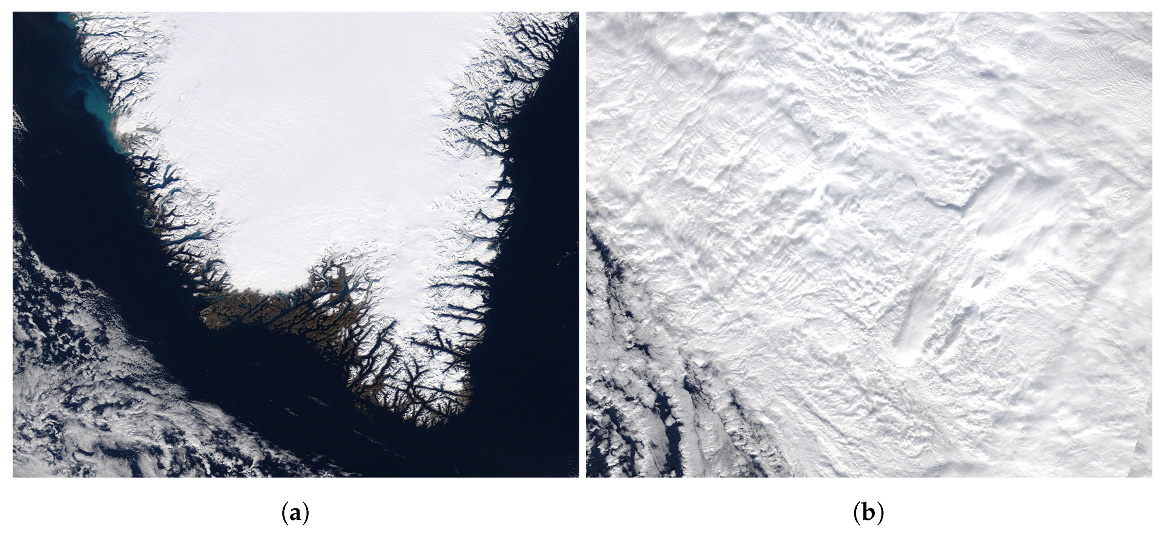
The presence of clouds also has implications for the ice-albedo feedback. We can readily see in satellite imagery that the contrast between ice-covered and open water is completely obscured by opaque cloud cover (Figure 1). Studies have found that the TOA albedo changes less in response to reduced surface cover than the surface albedo. Using observations from the Earth Radiation Budget Experiment (ERBE), Gorodetskaya et al. [8] found that sea ice and snow cover in high latitudes have reduced effectiveness, 0.22 and 0.16, respectively, on the TOA albedo. Kato et al. [16] also concluded that clouds reduced the effects of sea ice loss on reflected SW radiation at the TOA in the Arctic Soden et al. [17] found a roughly 30% reduction in surface albedo feedback kernels when using all-sky as opposed to clear-sky fluxes in global climate models. Hwang et al. [18] found that clouds reduced the surface albedo feedback radiative kernel over the Northern High Latitudes from 1.13 ± 0.44 Wm K to 0.49 ± 0.30 WmK from observations.
However, while our knowledge of Arctic cloud properties has improved over the past decades with increased satellite observations [19], the precise magnitude of the modulating influence of clouds is still unresolved. For example, the record low sea ice extent in 2007 was caused, in part, by the combination of reduced cloud cover and anomalously high solar absorption at the surface with an already weakened ice pack [20,21]. In response to Kay et al. [20], Graversen et al. [22] found that the ice-albedo feedback exacerbated sea ice melt but claimed the true cause of the low sea ice extent increased downward LW emission and turbulent fluxes from anomalously high atmospheric energy transport. Schweiger et al. [23] completely ruled out the negative cloud anomaly as contributing to the low sea ice minimum in 2007, and more recently Ding et al. [24] declared that trends in summer atmospheric circulation are the dominant drivers of sea ice decline during the satellite era. However, these latter studies used data from reanalyses that have been shown to exhibit biases in surface radiation in polar regions [25]. This study quantifies the modulation of TOA albedo and sea ice loss by clouds using satellite observations and compares the results with reanalyses.
The TOA albedo is influenced by both the surface and the atmosphere, the latter being heavily influenced by clouds [26]. Past studies have partitioned the TOA albedo into surface and atmospheric components both globally and at high latitudes [27,28]. Observations reveal that the atmosphere dominates the TOA albedo across the Earth, even in the Arctic where the surface albedo is quite high. Although the surface does not make the largest contribution to the TOA albedo, it is responsible for the majority of variability in the Arctic TOA albedo. From Qu and Hall [27], more than 50% of TOA albedo interannual variability is due to the changes in the surface albedo. Since the atmospheric contribution is dominated by clouds, the albedo partitioning scheme from [28], discussed in more detail later, can be further used to quantify the modulating effects of clouds on TOA albedo response to changing surface cover in the Arctic and evaluate their representation in reanalyses.
Reanalyses have been used extensively to study Arctic climate since they provide continuous temporal and spatial coverage as well as variables that can be difficult, if not impossible, to directly measure [29,30,31]. These challenges also mean that there are few measurements to validate reanalyses in the Arctic because there are relatively few in situ observations in this remote and harsh region. However, some recent studies have found large biases in reanalyses for cloud properties, including cloud fraction, liquid water path, and ice water path, when compared with available ground and satellite observations [32,33,34,35]. Such discrepancies are intertwined with surface radiative biases, where reanalyses still struggle to match observations in the Arctic [36,37,38]. Cao et al. [39] investigated the representation and trends of surface and TOA albedos in four reanalyses, finding that none accurately captured the decline of albedo in recent decades. Yet Cao et al. [39] only compared surface albedos on annual and seasonal scales. Other studies have looked at planetary albedo, but the ability of reanalyses to correctly partition the TOA albedo into surface and atmospheric components has not been studied.
This work seeks to answer two fundamental questions: How do clouds modulate the impact of surface cover changes on the TOA albedo? And how well are these effects captured in modern reanalyses that are often used in polar climate studies? We partition the surface based on sea ice and snow cover to show the effects of surface cover on the energy balance over a time period with large surface cover variability. The surface partitioning is further applied to the TOA albedo and its contributions to show their sensitivities to changes in surface cover. We use new metrics to quantify the effects of clouds on the TOA albedo by comparing the all-sky and clear-sky TOA albedo contributions. These metrics are further used to evaluate five modern reanalyses in their representations of clouds and surface cover feedbacks in the Arctic.
2. Methods
2.1. Datasets
This study uses the Arctic Observations and Reanalysis Integrated System (ArORIS), a collection of satellite, in situ and reanalysis datasets focused on the Arctic and created to support Arctic climate research [40]. All data in ArORIS is re-gridded to a uniform 2.5° × 2.5° grid and averaged to monthly timescales. We use radiative fluxes from the Clouds and Earth’s Radiant Energy System Energy Balance and Filled (CERES-EBAF) version 2.8 on board the Terra and Aqua NASA satellites. TOA fluxes in the CERES-EBAF dataset are adjusted within their ranges of uncertainty to be consistent with global ocean heat uptake from in situ ocean observations [41]. Errors in gridded down-welling SW fluxes at the TOA are 0.5 Wm and 5 Wm in outgoing all-sky SW irradiance for January–June 2002 and 4 Wm thereafter [42,43]. Outgoing clear-sky SW irradiance has an estimated error of 2.6 Wm. At the surface, uncertainties are 11 Wm in both down-welling and reflected SW fluxes [44]. Total cloud fraction is derived from the CloudSat 2B-GEOPROF-LiDAR product that uses a combination of Cloud Profiling Radar (CPR) and Cloud-Aerosol LiDAR with Orthogonal Polarization (CALIOP) observations. These active sensors can detect clouds over bright surfaces and surface inversions that are common in the Arctic [45,46]. CloudSat/CALIPSO data are only available for 2007–2010 over 82° S–82° N.
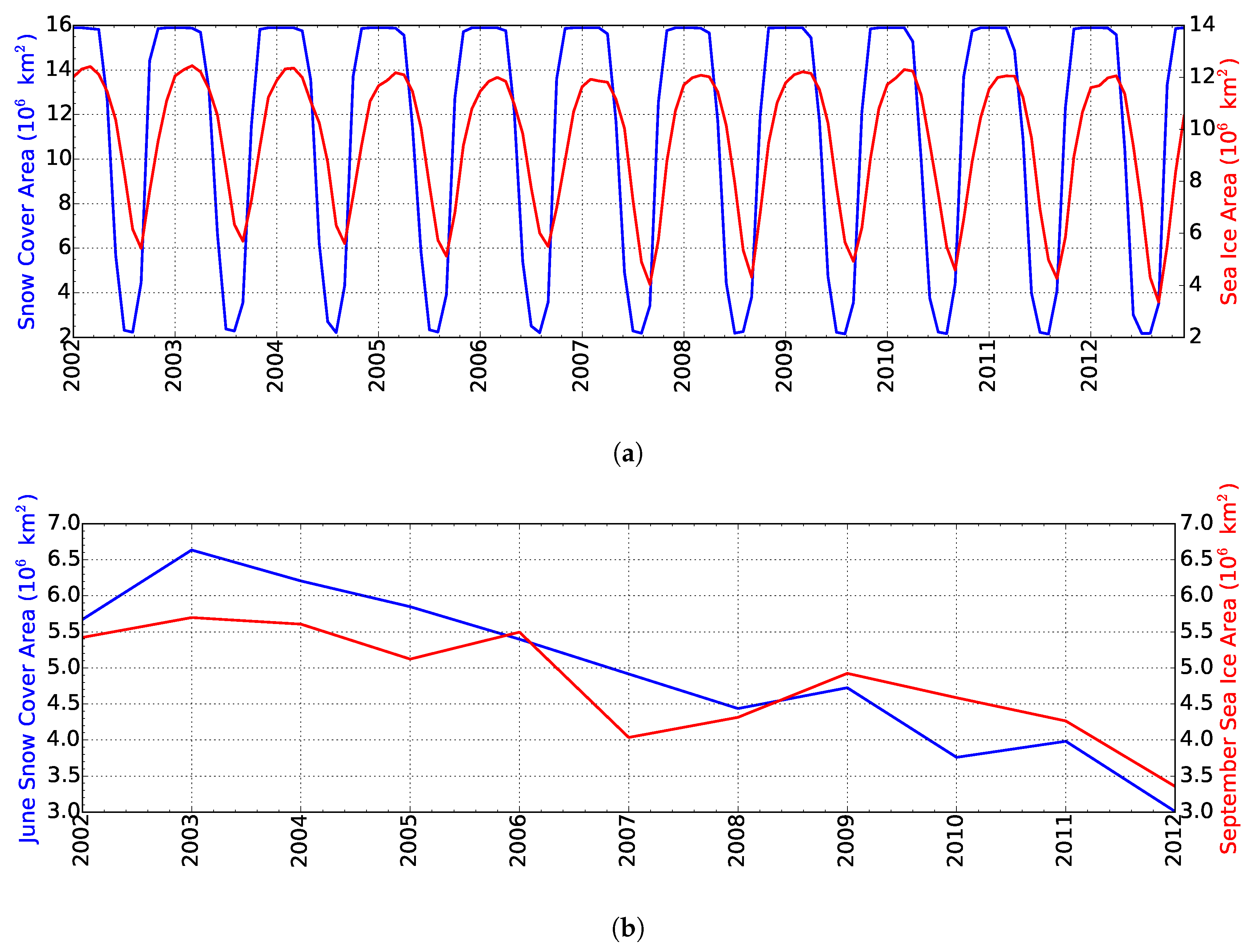
Surface ice and snow cover variables derive from the National Snow and Ice Data Center (NSIDC) Equal-Area Scalable Earth grid (EASE) weekly product. A long-term record of sea ice concentration (SIC) dating back to 1979 is estimated using brightness temperature from the Nimbus-7 Scanning Multichannel Microwave Radiometer (SMMR), the Defense Meteorological Satellite Program (DMSP) -F8, -F11 and -F13 Special Sensor Microwave/Imagers (SSM/Is), and the DMSP-F17 Special Sensor Microwave Imager/Sounder (SSMIS). The EASE weekly product also summarizes snow cover over land. Snow cover fraction (SCF) is created when grid cells flagged as snow-covered (defined as ≥50% snow cover of the original 25 km grid cell) are interpolated from the EASE grid to larger grid cells. For this work we use the years 2002–2012, corresponding to the period for which CERES is available in ArORIS. This period spans a time of high sea ice variability when the September minimum sea ice extent has ranged from 3.4 to 6.0 million km. Figure 2 shows the variability of monthly sea ice and snow cover areas as well as the decline of June snow cover area and September sea ice area over 2002–2012.
2.2. Reanalyses
Relationships between albedos, clouds and surface cover derived from the above observations are compared to five reanalyses: European Center for Medium-Range Weather Forecasting (ECMWF) Interim (ERA-Interim), Modern-Era Retrospective Analysis for Research and Applications 2 (MERRA-2), National Center for Environmental Prediction/Department of Energy reanalysis 2 (NCEP R2), and the Arctic System Reanalysis versions 1 and 2 (ASRv1 and ASRv2). A summary of the specific reanalyses parameters used in this study is given in Table 1.
ERA-Interim is an ECMWF global reanalysis based on ERA-40 [47] that uses a four-dimensional variable assimilation (4D var) [48]. Sea ice albedos in ERA-Interim are monthly values based on Ebert and Curry [49] that are interpolated to the forecast time. Bare sea ice is assumed to represent the summer sea ice values, and the dry snow albedo is used for winter. SIC is assimilated from NCEP real-time global (RTG) for January 2002–January 2009 and Operational Sea Surface Temperature (SST) and Sea Ice Analysis (OSTIA) for February 2009 to present. In ERA-Interim, SCF is a function of snow water equivalent () and snow density, :
Only net clear-sky fluxes are available for ERA-Interim. To calculate the up-welling and down-welling clear-sky SW fluxes at the surface, surface albedo, , is calculated from the all-sky fluxes at the surface,
and is used to solve for the desired flux components. While this is the suggested method [50], it is noted that the results are not precisely what is produced by the model because of differences in direct and diffuse shortwave radiation due to the absence of clouds. As with all reanalyses used here, ERA-Interim does not directly assimilate cloud observations. It uses prognostic equations for cloud liquid water and ice and cloud fraction from a three-class two-moment scheme [51,52]. Clouds are assumed to be maximum-random overlapped.
MERRA-2 is the continuation of MERRA [53], which includes enhancements to the meteorological assimilation, the Goddard Earth Observing System (GEOS) model, and the representation of ice sheets [54]. In MERRA-2, the sea ice albedo varies seasonally based on flux tower observations from the Surface Heat Budget of the Arctic Ocean (SHEBA) field campaign [55]. Monthly values are calculated from SHEBA and interpolated to instantaneous values. SIC is prescribed from various ocean datasets [56]. Glaciated surfaces (e.g., Greenland) have dynamic energy and hydrologic properties that allow snow densification, meltwater runoff, percolation, and refreezing to be represented. The glacial model used includes updates to the NASA Catchment land surface model for snow cover, which has a prognostic surface albedo variable. MERRA-2 also includes a prognostic cloud scheme from [57] and assumes cloud are maximum-random overlapped.
NCEP R2 is an updated version of NCEP [58] correcting known errors, including sea ice and snow cover representation. These now follow the sea ice specifications of AMP-II [59]. Snow cover is interpolated from the NSIDC weekly EASE-grid product to daily values, and the model is forced to match observations. For permanent snow, the albedo is set to 0.75 for latitudes above 70° and 0.6 for lower latitudes with a snow depth of at least 1 cm. NCEP R2 also updated several parametrizations of physical processes, including the radiative transfer model. However, NCEP R2 does not have clear-sky radiative fluxes available, which limits the analysis of radiative cloud effects. NCEP R2 uses a diagnostic cloud scheme with a parameterized relative humidity-cloud cover relationship and assumes random overlap.
Finally, ASR is a high-resolution regional reanalyses for the Arctic using an optimized version of the Polar Weather Research and Forecast (PWRF) model with ERA-Interim data for initial and lateral boundary conditions [60,61]. We compare versions 1 and 2 in this study. ASR employs the Noah Land Surface Model (LSM) with several improvements, including fractional sea ice within each grid cell and specified sea ice characteristics (e.g., thickness, snow cover over sea ice, albedo). Sea ice fractions are prescribed from daily NSIDC SSMI/I microwave radiometer measurements for the Polar WRF model. These prescribed values include first-order seasonal variations for the Arctic Ocean that depend on latitude and time of year. A seasonal cycle is used for the sea ice albedo which varies annually based on melt/freeze dates from satellite observations. Snow cover and snow albedo are assimilated from the National Environmental Satellite, Data, and Information Service (NESDIS) observations and vary seasonally, again, to represent melting and freezing. ASRv1 uses the PWRF single-moment five-class microphysics scheme, and ASRv2 uses the PWRF two-moment Morrison scheme. 2D total cloud fraction is not readily available in either version.
2.3. Surface Partitioning
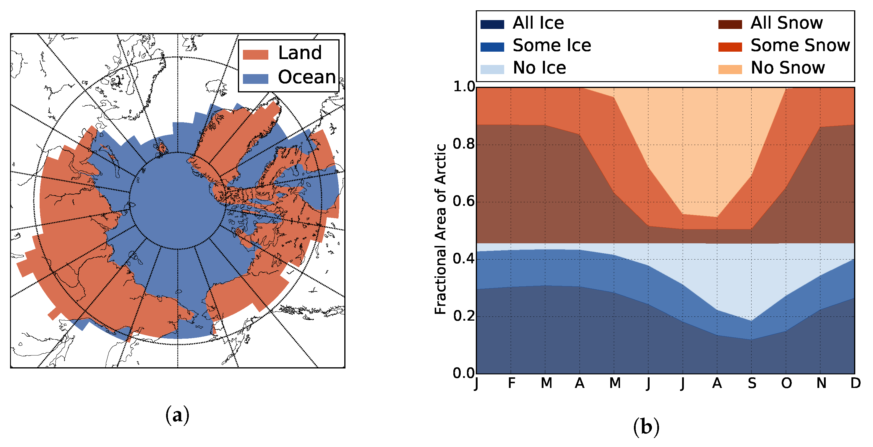
The goal of this work is to quantify the extent to which cloud cover modulates how the TOA albedo responds to changing sea ice and snow cover. This requires definitions of the Arctic and the areas covered by ice and snow. In this study, the Arctic is defined based on the mean 2-m air temperature from the Atmospheric Infrared Sounder (AIRS) on the Aqua satellite for 2002–2015. 2.5° × 2.5° grid cells in the NH with an annual mean temperature at or below 0 °C are considered part of the Arctic, as shown in Figure 3a. Defining the Arctic with this method removes most of the warm waters from the Atlantic Ocean that remain ice free throughout the year and behave differently than the majority of the Arctic [62]. There are various definitions of the Arctic, including area north of the Arctic circle (66.5° N), other latitudes at or above 60° N, the Arctic tree line, or the 10 °C July isotherm [63,64]. Our definition of the Arctic bears resemblance to the latter two definitions. Using this Arctic definition, grid cells considered ocean (defined as having a land fraction less than 0.5) are further divided into three categories based on the SIC: all sea ice for SIC > 0.85, no sea ice for SIC ≤ 0.15, and some sea ice for values between these limits. The same conditions are used to characterize land grid cells based on SCF. Please note that no further delineation between different types of sea ice- or snow-covered surfaces is made here (e.g., snow-covered ice or surface melt ponds). While the albedos of these surfaces can vary significantly, the objective of this study is to document the aggregate impacts of these surfaces on albedos. The mean annual cycle of these surface partitions over 2002–2012 are shown in Figure 3b. Sea ice has the expected minimum in September and maximum in March with at least a small area of open water present throughout the year. Snow cover leads sea ice by one to two months, reaching a minimum in July and August. The area covered by some or all snow is fairly constant the rest of the year, and bare land is only present May–October. This partitioning will be used to isolate the contributions of ice- and snow-covered surfaces to the TOA albedo, determine the roles clouds play in modulating these effects, and assess how well reanalyses capture these relationships.
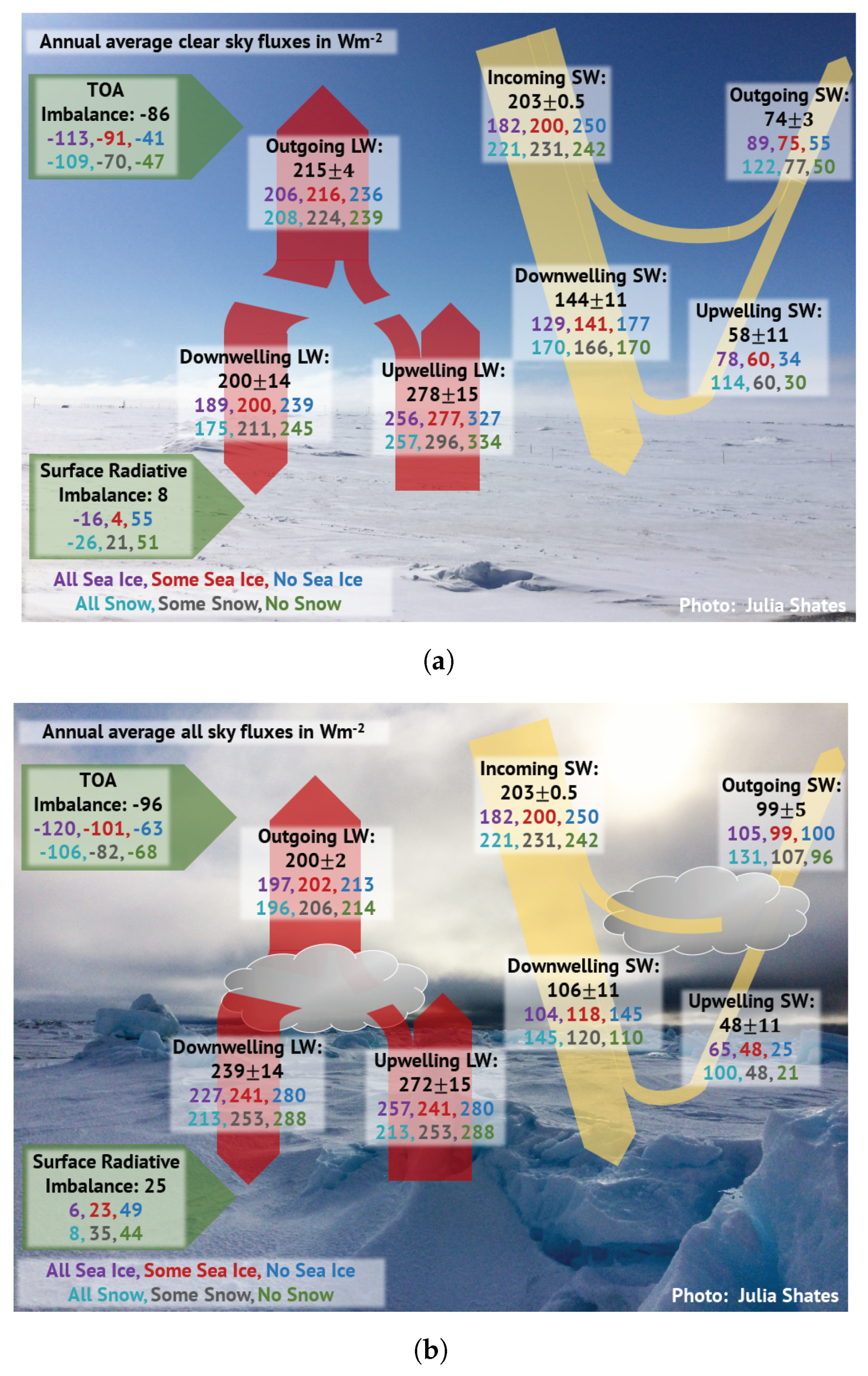
To set the stage for determining responses to surface cover variations, Figure 4 decomposes the annual mean Arctic radiative energy budget from CERES observations into each surface type for the period 2002–2012. Both diagrams show marked differences in surface up-welling SW fluxes between surface types. In the all-sky energy budget (Figure 4b), the difference in up-welling SW over open ocean and over ice-covered ocean is 40 Wm, and the difference between bare land and snow-covered land is 79 Wm. Similar differences are observed in clear skies (Figure 4a) where the sea ice increases the up-welling SW relative to open water by 44 Wm while snow cover increases up-welling SW by 74 Wm relative to bare land. However, the TOA energy budget tells a different story. Figure 4b suggests that the effects of surface cover on TOA fluxes are muted in the presence of clouds. The difference in outgoing SW between open water and ice-covered ocean is only 5 Wm, in Figure 4b as opposed to 34 Wm in Figure 4a. Likewise, the difference between bare and snow-covered land is reduced from 72 Wm in clear skies to 35 Wm when cloudy skies are included. Clearly clouds play an important role in modulating SW radiation in the Arctic.
2.4. Albedo Partitioning
To quantify the effects of clouds in modulating surface cover on TOA albedo, we partition the TOA albedo into surface and atmospheric components using the method of Donohoe and Battisti [28]. The reader is referred to that study for a detailed derivation. In this framework, each grid cell is considered as having a single atmospheric layer over an underlying reflective surface. The model accounts for three SW radiation processes: atmospheric absorption, atmospheric reflection, and surface reflection. All three processes are assumed isotropic. Surface and TOA albedos can each be calculated by applying Equation (2) at the appropriate boundary. The TOA albedo is then partitioned into two contributions, one from the atmosphere and one from the surface. The atmospheric contribution, , is equal to the direct reflectance, R, of SW radiation by the atmosphere,
The surface contribution to the TOA albedo, , encompasses the amount of SW radiation that is reflected by the surface and passes through the atmosphere, eventually exiting at the TOA, including the effects of multiple reflections between the atmosphere and surface
where A is the atmospheric absorption
Together, the atmospheric and surface contributions sum to the TOA albedo as calculated by Equation (2). Partitioning the TOA albedo in this way allows the impacts of changing surface conditions and atmospheric constituents on the planetary albedo to be separated.
To further isolate the effects of clouds on this partitioning, we can take the difference between each contribution to the TOA albedo for all-sky and clear-sky conditions. Multiplying this difference by the solar insolation at the TOA converts it into flux units. Mathematically, the difference between all- and clear-sky TOA albedos multiplied by incoming SW is equivalent to the SW cloud radiative effect (CRE) (with the opposite sign):
remembering that . Thus, the partitioning of TOA albedo into its two contributions, in all- and clear-sky conditions, is directly related to SW CRE, but the method also allows direct evaluation of the impact of surface conditions on TOA radiation. The difference in atmospheric contributions represents the amount of reflected SW radiation due to clouds at the TOA, and the difference in surface contributions represents the amount of SW flux that would have been reflected by the surface under clear-sky conditions [26]. We apply this framework to investigate the dependence of each of the aforementioned quantities on sea ice and snow cover.
3. How Does Planetary Albedo Respond to Surface Cover?
3.1. Effects of Surface Cover on TOA Albedo
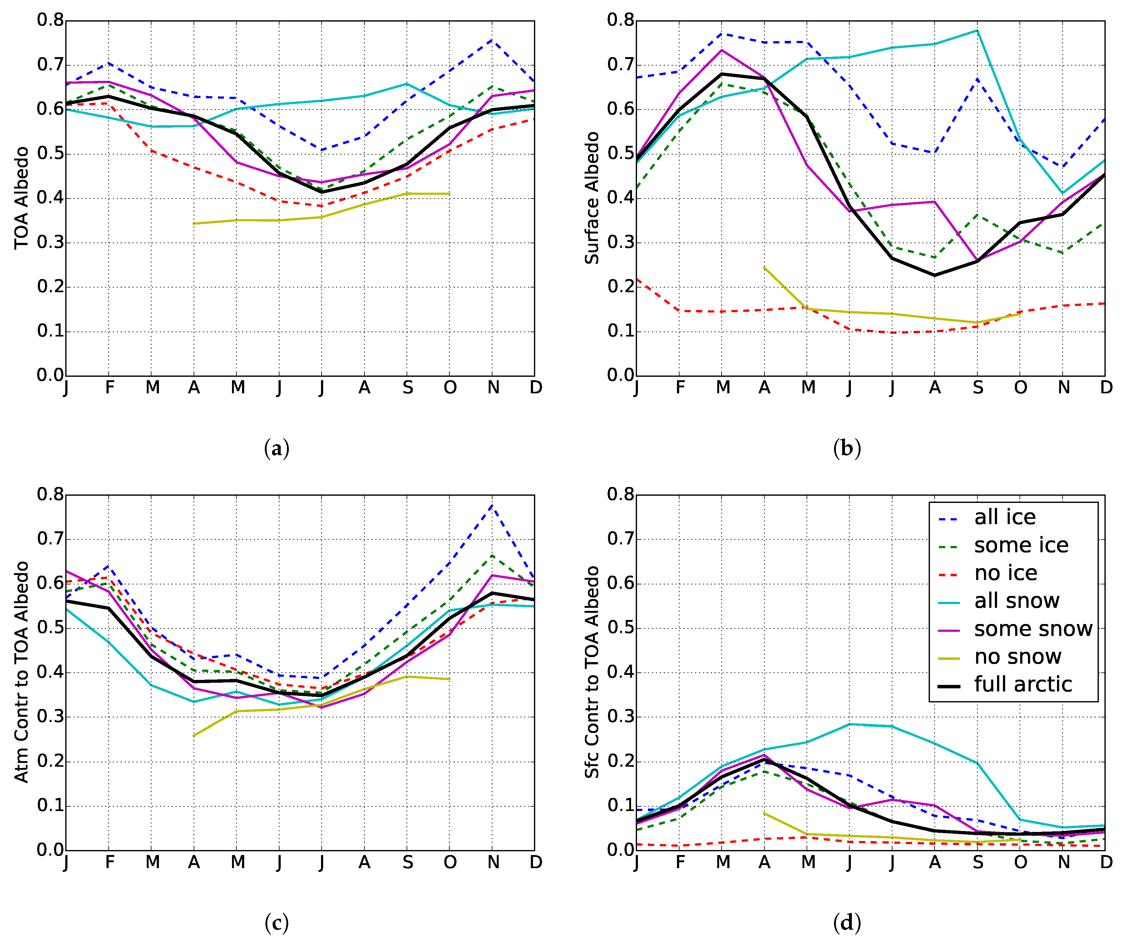
The surface and planetary albedos exhibit distinct annual cycles that depend on surface type. Mean monthly albedos over the Arctic domain for 2002–2012 calculated from CERES all-sky fluxes are shown in Figure 5 for each surface condition. The Arctic-mean surface albedo reaches a peak of 0.68 in March when snow and sea ice cover are both at their maxima. Surface albedo decreases with snow/ice cover throughout the summer reaching a minimum of 0.23 in August, approximately one third of the spring maximum. Spatially, (Figure 6) the exposed land and open ocean have much lower albedos once sea ice and snow melt. Evidence of surface melt is seen in the central Arctic ocean beginning in June where observed surface albedo decreases despite the high SIC. Land areas with high SCF through the summer, e.g., the Greenland ice sheet (GIS), maintain high surface albedos, >0.8, throughout the year due to their perpetually glaciated surfaces. They are the brightest surfaces from June to October.
The TOA albedo has a markedly different annual cycle than that of the surface. In Figure 5, the TOA albedo peaks in February and is at a minimum in July, leading the surface albedo by a month. Furthermore, the amplitude of the annual cycle is dramatically reduced: the February (0.63) and December (0.61) maxima are less than the maximum surface albedo, and only 50% larger than the July minimum (0.41), which is almost twice as large as the minimum surface albedo. The TOA albedo also varies less spatially across the Arctic than the surface albedo, seen in Figure 6. While the enhanced reflection from the GIS and the sea ice extent in the central Arctic ocean are visible at the TOA, these signals are less pronounced and the strong contrasts between open ocean and sea ice seen at the surface are muted at the TOA.
These findings are consistent with previous work that has shown that the TOA albedo is dominated by the atmospheric contribution (i.e., clouds) that masks the surface albedo [27,28]. Figure 5 demonstrates that, without exception, the atmospheric contribution to the TOA albedo is consistently larger than that of the surface, even over the brightest surfaces (e.g., GIS) throughout the year. The atmospheric contribution therefore dominates the seasonal cycle of TOA albedo, rising to 0.58 in winter and falling to 0.35 in July, accounting for an average 84% of the TOA albedo. As with the TOA albedo, the atmospheric contribution is also much less varied spatially across the Arctic than the surface albedo (Figure 6), although there is still contrast between land and ocean in early spring.
Although the surface contribution to the TOA albedo is proportional to the surface albedo, its average annual behavior is quite different. The spring peak has a maximum of 0.21 in April when surface ice and snow cover are high and cloud cover is relatively low [65,66], contributing 35% of the TOA albedo. By June, the surface contribution decreases to 0.1, about 10% of the TOA albedo, when snow on land has largely receded, and remains low for the remainder of the year. These surface contributions are 2–3 times smaller than the actual surface albedo. As the surface albedo decreases, clouds play an increasingly dominant role in defining the TOA albedo since the surface reflects less SW radiation. The one exception to this trend is the GIS where the surface contribution increases to 0.28 in summer relative to spring and fall. This is likely a result of the fact that as wetter snow at mid-latitudes recedes, snow cover in the summer is dominated by the high-altitude, brighter snow on the GIS.
Figure 5 and Figure 6 both clearly indicate that the large differences in surface albedo between the different surface partitions are muted at the TOA. The surface albedos for fully ice- and snow-covered surfaces are roughly 3–5 times greater than ice- and snow-less surfaces in all months when these surfaces are present (as seen in Figure 3b, on average, land without snow is only present April through September). Conversely, the TOA albedo over snow- and ice-covered surfaces are at most 1.7 times larger than their bare counterparts. The differences in surface albedo are being masked by clouds.
The contributions to TOA albedo also have notably different behaviors across the different surfaces. The surface contribution to the TOA albedo shows similar patterns to the surface albedo across surface types: uncovered ocean and land are low throughout the year; partially covered ocean and land follow the Arctic-wide average; and fully snow-covered land is larger than all other surfaces through the summer. Although the surface contribution has small absolute differences relative to other albedos, the maximum difference between surface contributions is a factor of 13 greater between snow-covered land (0.27) and open ocean (0.02) in the summer. In contrast to the surface contribution, the atmospheric contribution behaves similarly for all surface types throughout the year. The maximum difference between atmospheric contributions is only a factor 1.33 between 0.3 (land with no snow) and 0.4 (ice-covered ocean) during the summer, a fractional difference ten times less than the surface contribution. This shows that the atmospheric contribution has reduced dependence on the underlying surface.
Comparing Figure 5 and Figure 6, the relative roles of the atmosphere and surface contributions to the TOA albedo variability can be summarized as follows: the annual cycle of Arctic-wide average TOA albedo is dominated by the annual cycle of the atmospheric contribution while the surface contribution is responsible for variations in the spatial pattern of TOA albedo between surface types. This is clear since the TOA albedo over most surfaces, except for snow-covered land surfaces, exhibit similar annual cycles as the Arctic-mean (and the atmospheric contribution). Snow-covered land has a larger TOA albedo during summer when the Arctic overall sees a decrease; however, the peak at the TOA (0.61) is still damped compared to at the surface (0.78).
3.2. Cloud Modulation of Ice-Albedo Relationships
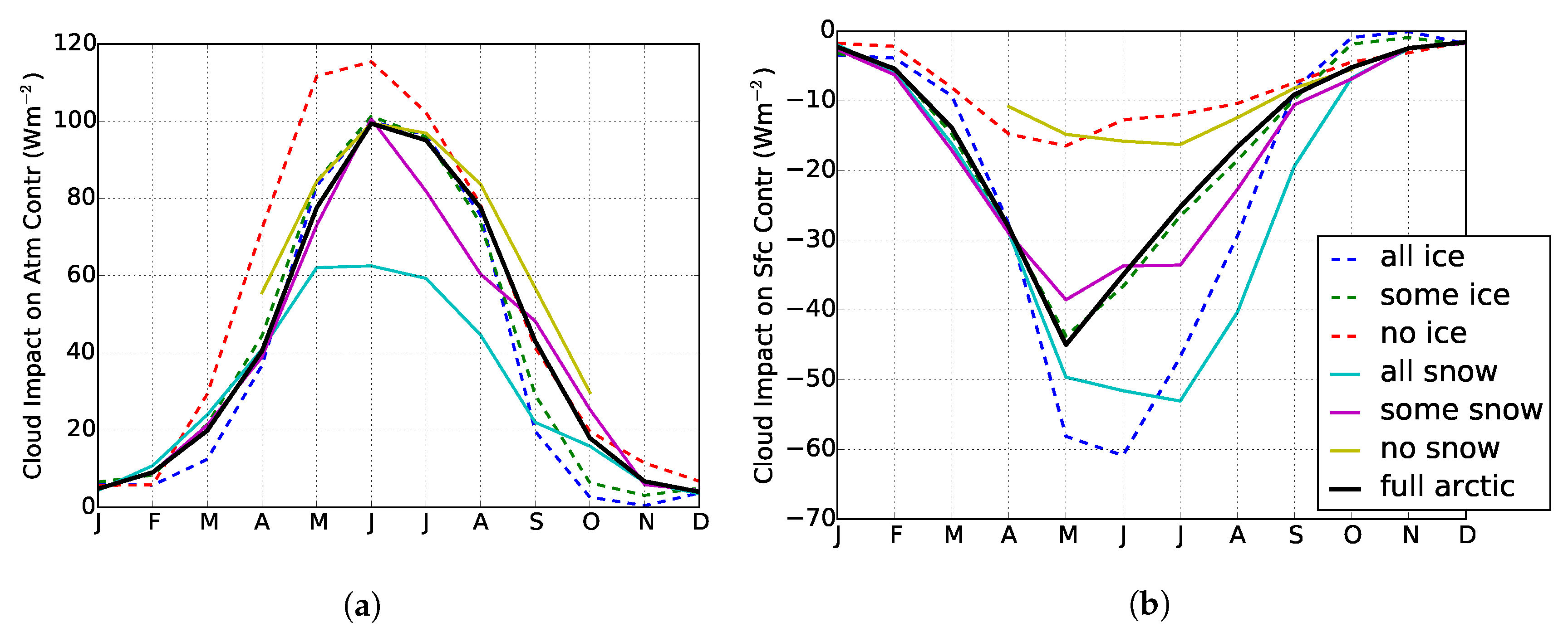
To cast these atmospheric effects into energetic units, the difference between all-sky and clear-sky contributions is multiplied by TOA solar insolation, giving the cloud impacts on surface and atmospheric contributions to TOA albedo. Recall that the difference between all- and clear-sky atmospheric contributions represents the amount of reflected SW radiation owing to clouds, and the difference for surface contributions shows the amount of SW radiation that would have been reflected at the surface if clouds were not present. When summed together these cloud effect contributions have the same magnitude as the TOA SW CRE, which is opposite in sign to TOA LW CRE and larger April through September.
The atmospheric contribution cloud impact (Figure 7a) follows the cycle of solar insolation with near zero reflection in winter and a June maximum of 100 Wm for the Arctic-wide average. The different surface types follow the same pattern as the Arctic average, but surface cover clearly exerts a strong influence on the magnitude of reflected SW due to clouds. During months with significant solar insolation, clouds exert a much stronger influence over less reflective surfaces. For example, clouds reflect nearly twice as much SW radiation over open ocean in June (115 Wm) than over land with all snow (62 Wm). It is this compensating cloud effect that explains how the atmospheric contribution dominates the TOA albedo while itself having negligible dependence on surface cover.
This result is illustrated more directly by the cloud impact on surface contribution in Figure 7b. In general, clouds reduce the surface contribution to TOA albedo because they block radiation reflected at the surface from reaching the TOA, but this effect is much more pronounced over brighter surfaces that reflect more SW radiation in the absence of clouds. The overall magnitude of this cloud masking effect is 5–6 times larger over ice- and snow-covered surfaces than open water or bare land. Collectively these analyses quantify two important effects: the extent to which surface conditions modulate clouds effects on the planet’s albedo and the masking influence of clouds on the effect of surface albedo changes on SW absorption.
While different surfaces have a strong influence on surface albedo, clouds significantly reduce the magnitude of these variations across the seasonal cycle. From a climate perspective, this leads us to ask: to what extent do clouds further modulate the ice-albedo feedback on longer timescales? While the length of the data record examined here is too short to examine trends, the large variations in SIC (Figure 2) over the period examined allow the impacts of clouds on year-to-year surface cover variations to be quantified.
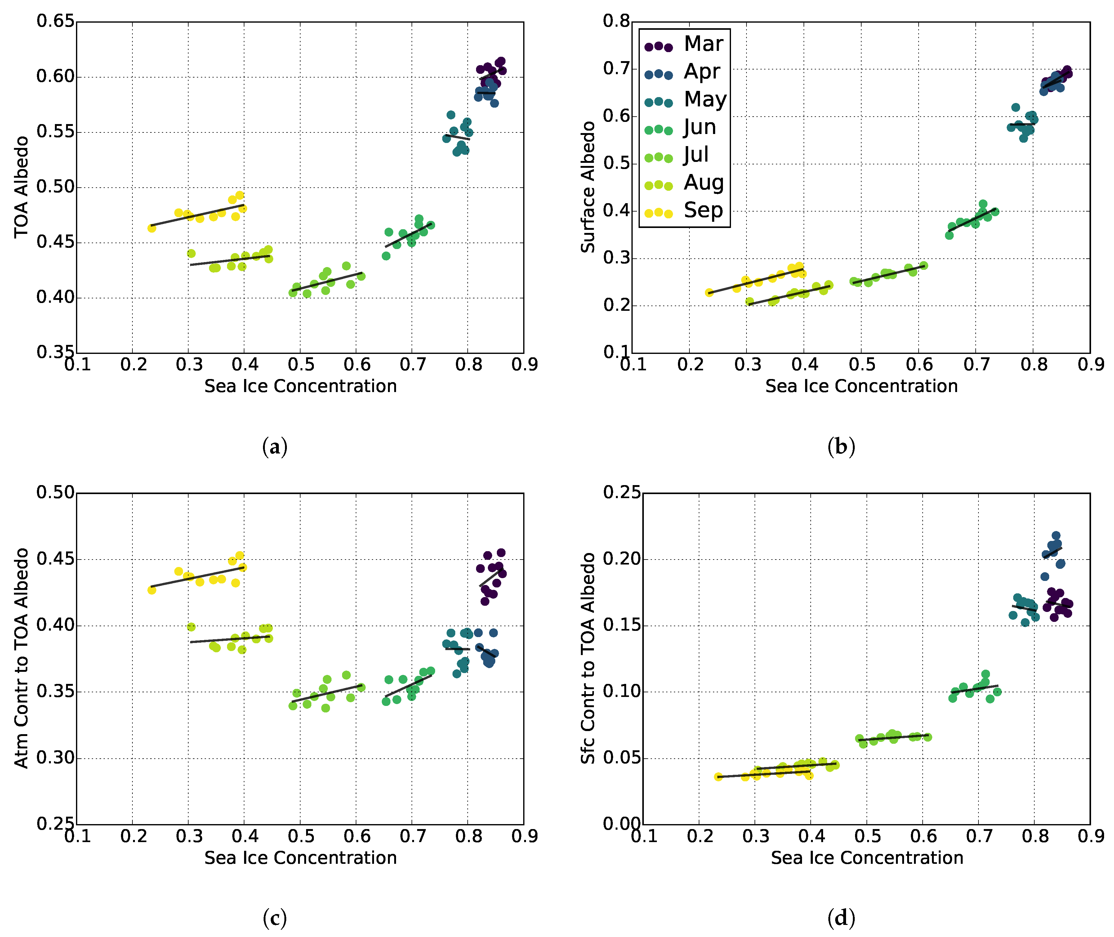
In pursuit of answering this question, we examine the response of monthly mean Arctic albedos and the TOA albedo contributions to average SIC and SCF for March through September in Figure 8 and Figure 9. In each month, the surface albedo and the surface contribution both exhibit strong positive relationships with SIC as expected (Figure 8). Both surface albedo and TOA albedo decrease from March through July. From July to August the TOA albedo increases due to the increased atmospheric contribution during these months, as opposed to the surface albedo which is reduced further as sea ice approaches its September minimum. The atmospheric contribution has a parabolic shape that depends less on surface cover and more on clouds.
In addition to these larger patterns between albedos and SIC, there are also trends within individual months owing to interannual variations in SIC. Linear fits for each month reveal that the sensitivity of surface albedo to SIC is quite constant (∼0.3) July through September (Table 2). TOA albedos and average SIC have less spread and no consistent trends in early spring (March–May). Beginning in June, surface albedo increases linearly with SIC. The surface contribution also increases with SIC but exhibits smaller trends due to the cloud masking effects described above. Further evidence of these effects is observed in the much weaker variation of monthly mean TOA albedo with SIC. The atmospheric contribution is fairly constant after July. This indicates that clouds are not particularly sensitive to changes in surface cover, consistent with the findings of Kay et al. [19] who note that cloud feedbacks may be limited to fall in the Arctic.
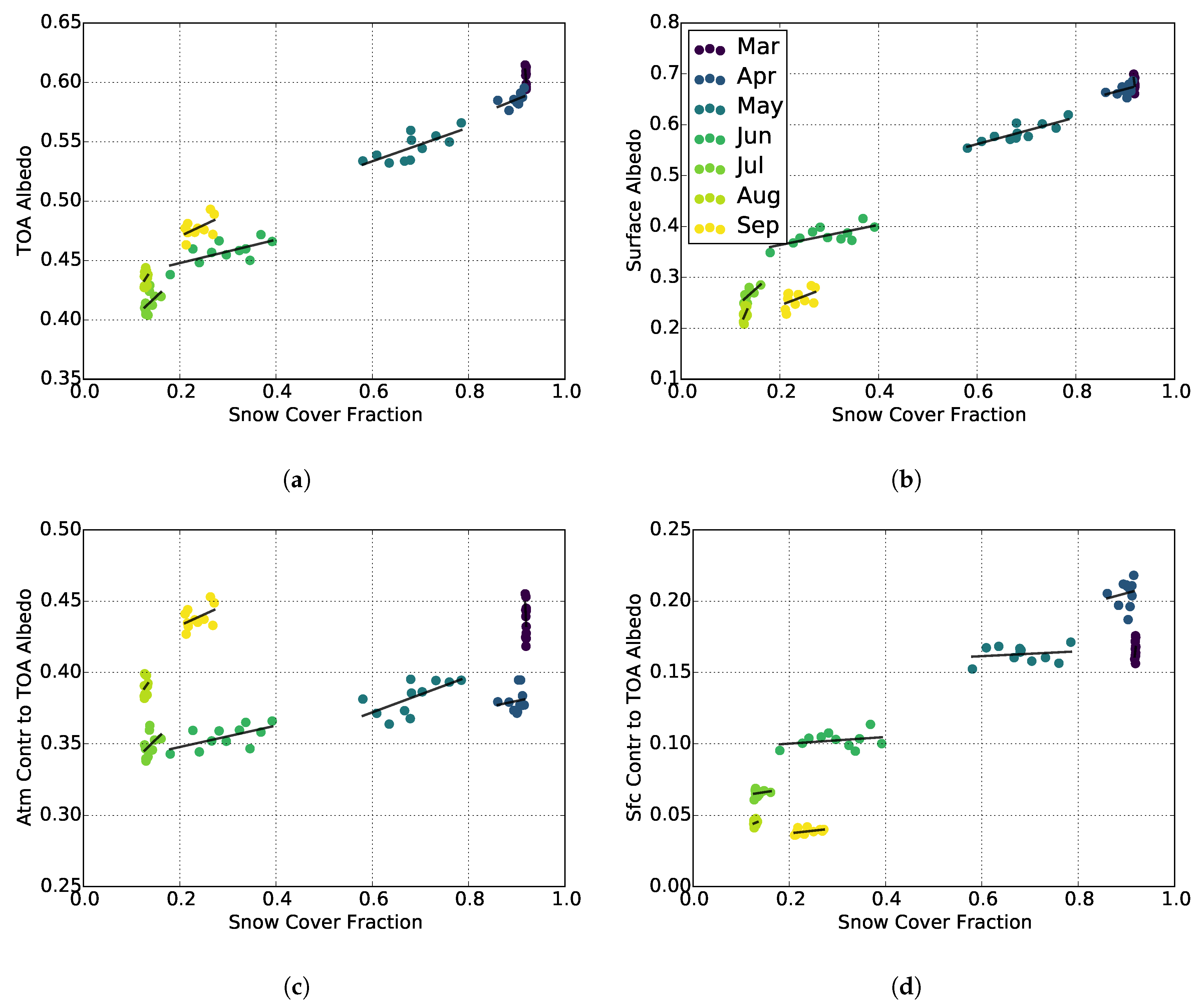
The relationships between albedos and SCF, Figure 9, are largely determined by the cycle of snow cover. The largest interannual variations in SCF occur in the melt season (May and June) and accumulation season (September). In May and June, the surface albedo decreases as the snow melts, with sensitivities of 0.26 and 0.20, respectively (Table 3). To a lesser extent, variations in the timing of snow cover accumulation in September lead to a similar relationship between surface albedo and SCF (0.37) but over a smaller range of SCF. Surface albedos in early spring and late summer have no significant relationship with SCF because there is either widespread snow cover or widespread bare land, as seen in Figure 6. The TOA albedo and its contributions follow this same pattern to varying degrees. TOA albedo has an overall linear relationship with SCF for March–September, but when focusing on individual months, May and June are again the months with statistically significant sensitivities, approximately half (0.14 and 0.10) those of the surface albedo. As with SIC, the surface contribution and surface albedo have similar patterns, but the surface contribution is roughly five to ten times smaller. The sensitivity of the atmospheric contribution is relatively large during May and June (0.12 and 0.07) but there is notable spread. While the TOA albedo is slightly more sensitive to SCF (0.16) than SIC (0.14) in May, by June SIC (0.25) has a stronger influence than SCF (0.10) at the TOA.
3.3. Representation in Reanalyses
Clearly clouds exert a significant influence on how strongly the effects of surface cover change influence the Arctic radiation balance. Reanalyses are also frequently used to study climate variations in this region of few observations. Given their pervasiveness in studying the Arctic regional processes and driving models [67,68], it is imperative to assess how well reanalyses capture the observed modulating effects of clouds.
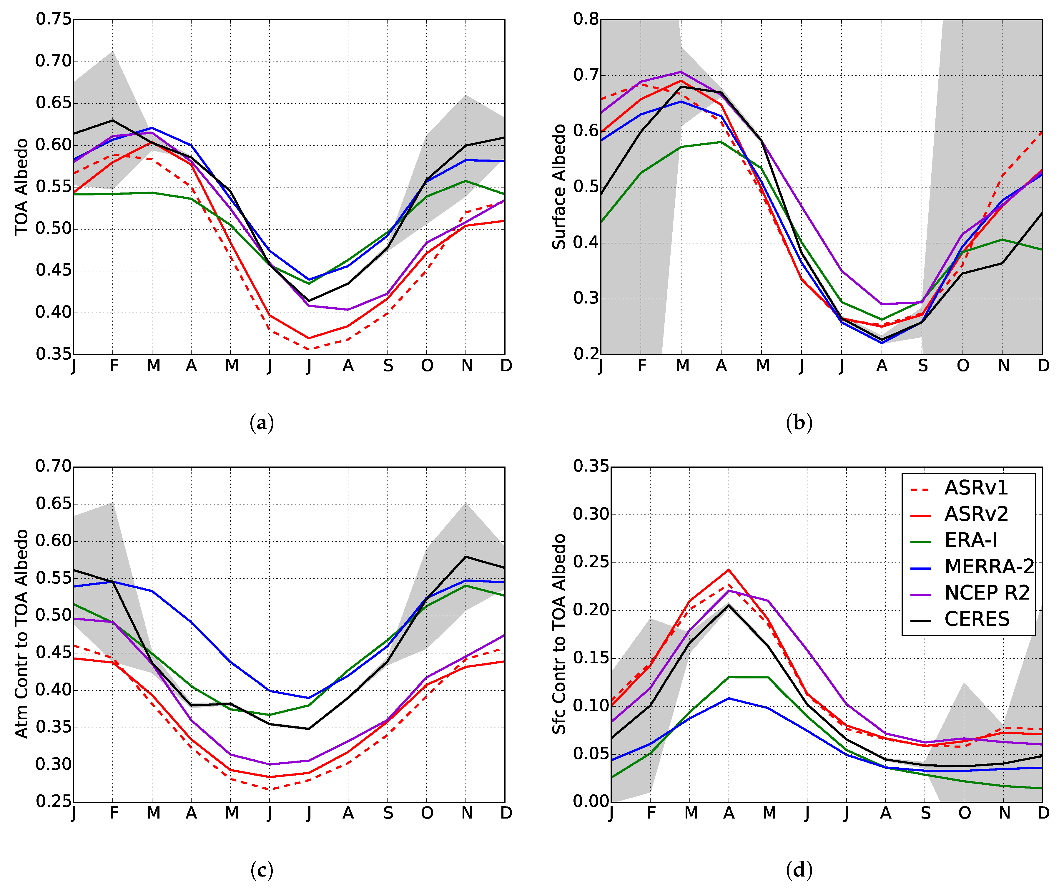
It is, therefore, important to ask how well reanalyses represent these cloud effects in the Arctic. The five reanalyses considered generally capture the shape of the annual albedo cycles but not necessarily their amplitudes. Given that a 0.05 difference in June albedo corresponds to 25 Wm difference in summer, biases of this magnitude are sufficient to exert a significant influence on surface processes, as noted by Cao et al. [39]. Winter months account for less than 5% of incoming SW radiation and have large errors in observations (Figure 10), so large biases during these months are less concerning than the rest of the year. In line with that fact, the largest differences in surface albedo occur in the winter, with over-estimations on the order of 0.10–0.20 but within the uncertainty of observations. The reanalyses perform better during the rest of the year, with surface albedo biases ranging from 0.01 (MERRA-2) to 0.1 (NCEP R2).
The spread in TOA albedo in the reanalyses is large in summer months owing primarily to the underestimation by ASR. ASRv2 moderately improves relative to ASRv1 but still underestimates TOA albedo by up to 0.08 (40 Wm) in the summer peak. The performance of the other reanalyses vary more by season. For example, ERA-Interim predicts a smaller annual cycle in TOA albedo than CERES, as well as surface albedo, while the minimum in NCEP R2 lags observations by a month.
Figure 10c demonstrates that the discrepancies in TOA albedo largely result from differences in the atmospheric contribution. The annual cycles of biases between reanalyses and observations map closely onto those in TOA albedo. ASRv1, ASRv2, and NCEP R2 underestimate the atmospheric contribution to TOA albedo for all months, while MERRA-2 and ERA-Interim overestimate it for all but the winter months. This is not necessarily surprising since the atmospheric contribution is dominated by clouds, which is a common problem for reanalyses [32].
Biases in the surface contribution to the TOA albedo are significant in spring when the spread in reanalyses approaches a factor of four. Both ASR versions and NCEP R2 represent the spring maximum in surface contribution relatively well, overestimating it by 0.05 or less. ERA-Interim and MERRA-2, on the other hand, underestimate the surface contribution to TOA albedo throughout the year with biases on the order of 0.1 (50%) during the spring maximum. This difference is enough to completely offset a positive bias in the atmospheric contribution in MERRA-2, artificially leading to a good agreement with observed TOA albedo that masks substantial biases in the partitioning of energy between the atmosphere and surface. In ERA-Interim, the large bias in springtime surface reflection leads to a substantial over-estimation of SW absorption in the spring (March–May).
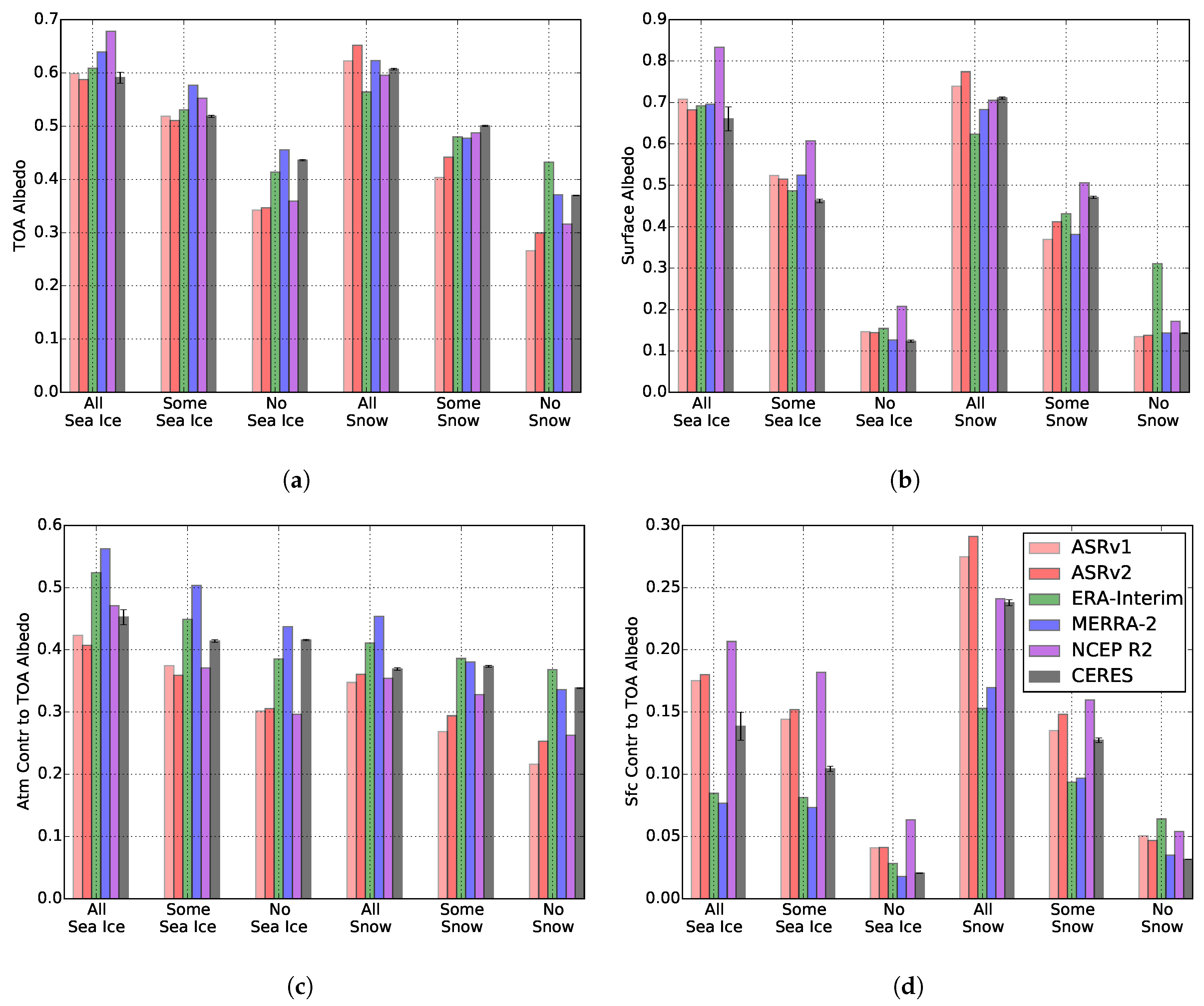
Figure 11 presents albedos and contributions averaged over March-September for each surface condition. Except for NCEP R2, which overestimates the albedo of all ocean surfaces, the reanalyses capture surface albedos for the surface partitions. Potentially more serious, however, are the biases in ERA-Interim over land with and without snow. ERA-Interim predicts an average surface albedo over land without snow (0.31) that is over twice that seen in observations (0.14). ERA-Interim also underestimates the surface albedo of snow-covered land (0.62 versus 0.71 in observations), which leads to a much lower contrast between land with and without snow (0.31) compared with observations (0.57). This suggests that the effects of snow cover changes may be significantly underestimated in ERA-Interim. In general, the other reanalyses represent variations in TOA albedo with surface conditions fairly well. The contributions to TOA albedo, however, are more widely spread relative to observations and each other. Both versions of ASR and NCEP R2 have positively biased surface contributions and negatively biased atmospheric contributions (≤0.1), compared to observations, that tend to cancel in the TOA albedo. Inversely, ERA-Interim and MERRA-2 have positive biases in atmospheric contributions that are compensated by negative biases in their surface contributions across most surface types. Thus, the apparent agreement in Figure 12a derives from a fortuitous cancellation of atmospheric and surface biases that have significant implications for how energy is partitioned between the atmosphere and surface in the reanalyses.
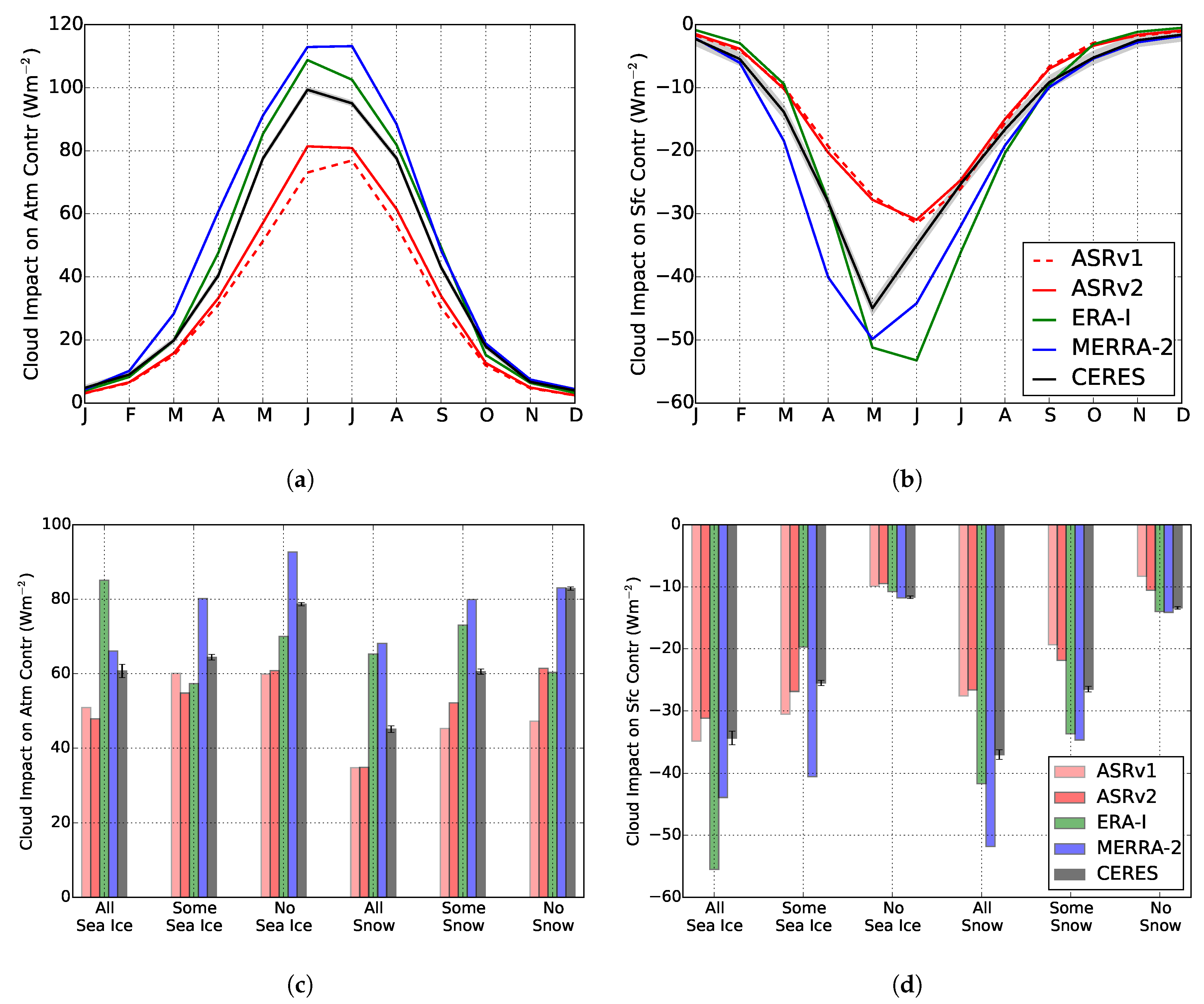
The observations suggest that clouds play an important role in moderating sea ice/snow cover albedo effects. To accurately predict surface warming and melt rates associated with climate responses, reanalyses must also capture these relationships between albedos and clouds. The biases in Figure 11c,d can be traced to errors in these relationships. While the three reanalyses with available clear-sky fluxes capture the annual cycle of cloud TOA albedo contributions in Figure 12a,b, they all vary in magnitude for the summer maximum, with a range of ±20 Wm for the atmospheric contribution and ±15 Wm for the surface contribution. The maxima and minima often lag observations by a month as well. This bias is also reflected at the TOA but is partially compensated by an enhanced atmospheric contribution.
When partitioned by surface type (Figure 12c,d), the three reanalyses exhibit mixed behaviors. MERRA-2 and both versions of ASR capture the cloud effects on atmospheric and surface TOA albedo contributions. ERA-Interim shows the opposite trend—the cloud impact on the atmospheric contribution is larger over sea ice than open water and there is no clear dependency of it on snow cover. All three reanalyses show that the surface contribution cloud effect increases with surface brightness, although ERA-Interim overestimates the change between high and low albedo surfaces by nearly a factor of two over oceans (45 Wm versus 23 Wm from CERES).
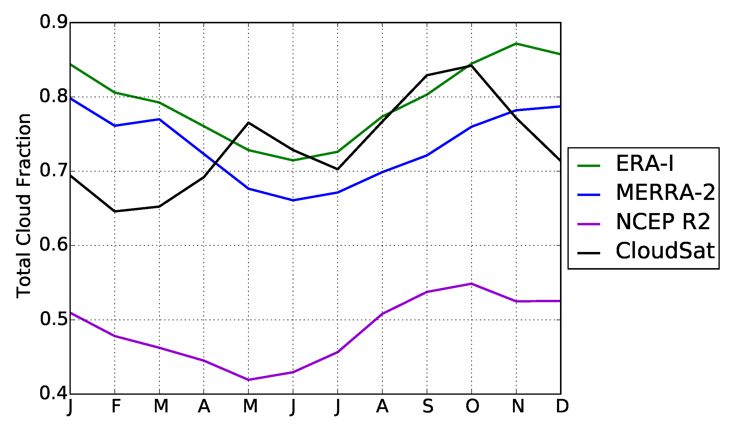
Some of the biases in reanalyses albedos can be attributed to their representations of clouds. Average cloud fraction over the Arctic up to 82° N is compared between CloudSat/CALIPSO and reanalyses, Figure 13. ERA-Interim matches observations fairly well May through October and overestimates the amount of clouds November through April. MERRA-2 is also near observations in summer and fall, although it underestimates cloud fraction during March-October and again overestimates cloud amount in winter. NCEP R2 underestimates cloud fraction for the entire year by 0.2–0.3. While none of these reanalyses directly assimilate cloud observations, the prognostic schemes used by ERA-Interim and MERRA-2 seem to perform better than the diagnostic cloud scheme from NCEP R2. The reader is directed to [34,35,69], for more detailed investigation of cloud representation in reanalyses.
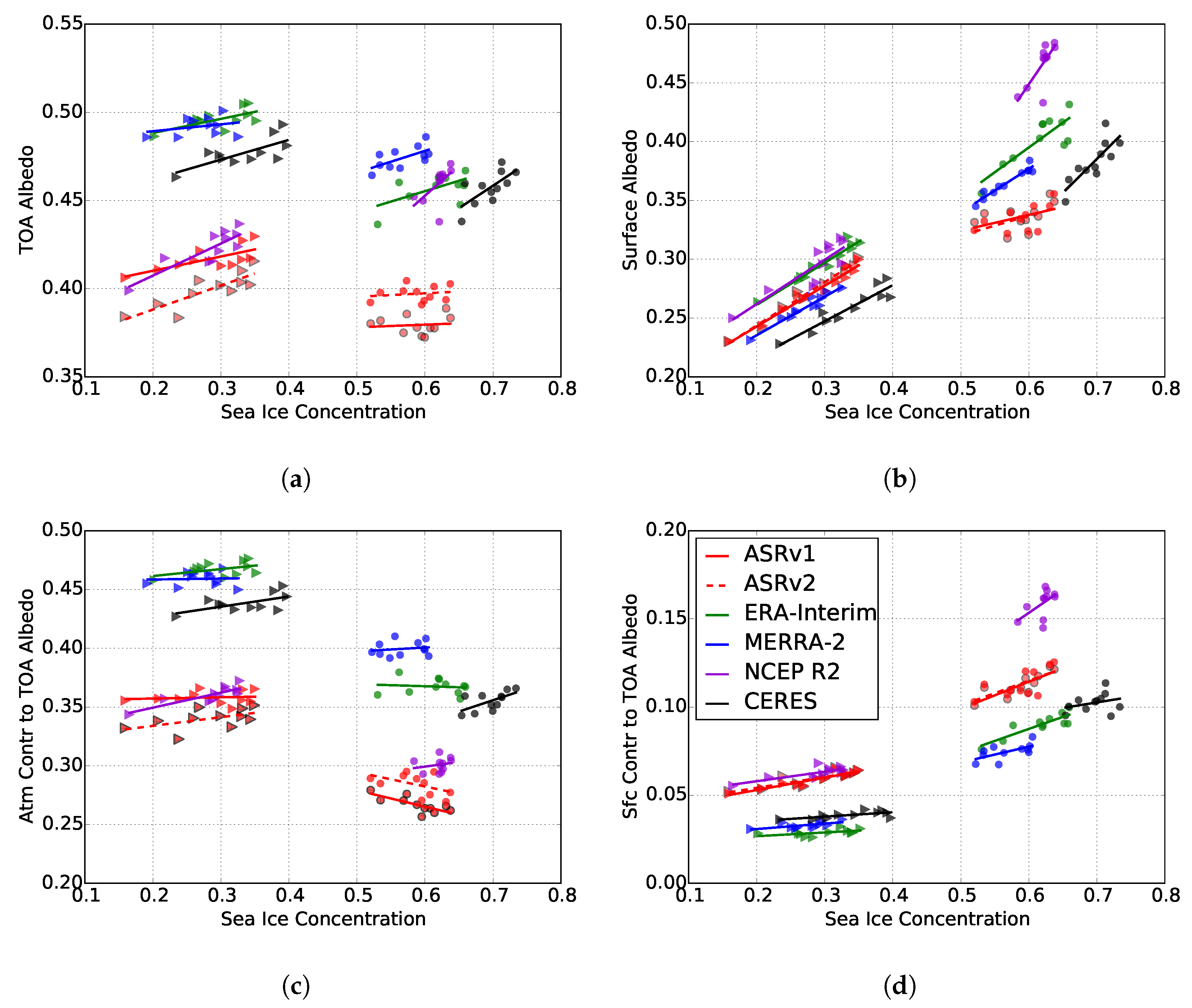
The reanalyses capture broad relationships between surface cover and albedos but struggle to accurately represent the relative magnitudes between different surfaces and TOA albedo contributions. To test the implications of these differences on the representation of interannual variability in the Arctic, the sensitivities of albedos and contributions to SIC in reanalyses and observations for June and September are presented in Figure 14 and Table 4. Surface albedo and surface contribution sensitivities to SIC are well represented by all five reanalyses in September and marginally less so in June. All reanalyses show that surface albedo is sensitive to SIC in June but have a range of 0.13 (ASR) to 0.85 (NCEP R2) with observations falling in the middle (0.57). Larger biases are present in the TOA albedo sensitivity to SIC. ASRv1 and ASRv2 show essentially no influence of SIC on the TOA albedo in June, contrary to observations. NCEP R2 tends to overestimate the influence of SIC on the TOA albedo. Reanalyses predict sensitivities closer to observations in September, although the MERRA-2 predicts no significant influence of SIC and NCEP R2 again overestimates the influence.
The differences between observations and reanalyses at the TOA can be found in the surface and atmospheric contributions. In June, all the reanalyses overestimate the influence of SIC on the surface contribution. They either underestimate its influence on the atmospheric contribution (MERRA-2, NCEP R2) or predict the opposite relationship (ASRv1, ASRv2, ERA-Interim). These competing biases result in greatly reduced TOA albedo sensitivity to sea ice, except for NCEP R2 that has a much larger surface contribution compared to observations. Most reanalyses are better aligned with observations in September when their biases in SIC influence on TOA albedo contributions are smaller.
4. Discussion and Conclusions
While Arctic amplification is an important component of climate change, the mechanics are not fully understood, particularly the effects of clouds. In this paper, we have quantified how clouds modulate albedos in the Arctic. The surface albedo changes with snow and sea ice cover through the seasons, but the TOA albedo varies only half as much. Reanalyses do not capture this relationship, generally predicting that SIC has less influence on the TOA albedo than seen in observations. In satellite observations, the atmosphere contributes 2–3 times more to the TOA albedo than the surface throughout the year. Clouds are the main contributor to the atmospheric contribution, increasing the atmospheric reflectivity and blocking SW reflected from the surface from leaving the Earth system. The atmospheric contribution to TOA albedo also depends less on the underlying surface, meaning that changes to the surface cover may have less impact on it. Despite differences in methods, our sensitivities are similar to the radiative effectiveness reported by [8].
The reduced sensitivity of TOA albedo to surface cover is important for the ice-albedo feedback. Our work supports previous studies that have found reduced ice-albedo feedback parameters due to clouds [17,18]. We have found that clouds mask the surface albedo and damp changes in surface cover at the TOA. When the surface albedo is sensitive to SIC changes in the summer and fall, the surface contribution to the TOA albedo is low, leading to reduced changes at the TOA. There is nuance, though. Clouds do not simply replace underlying snow and ice. While clouds have higher albedos than open ocean, there is still a measurable difference (∼0.15) in TOA albedo between land with and without snow cover and ocean with and without sea ice cover. Clouds may reduce the ice-albedo feedback, but the radiative effects of clouds at the TOA are unlikely to be large enough to prevent the ice-albedo feedback from continuing and contributing to Arctic amplification.
Since the interaction between clouds and albedos is essential to understanding and modeling the evolution of the Arctic, it is important that datasets used to study the Arctic, i.e., reanalyses, accurately portray these relationships. These results demonstrate that reanalyses cannot always be taken as proxies for observational datasets, especially in regions where limited observations are assimilated and for variables that cannot be directly measured. In such instances, models rely heavily upon parameterizations that are frequently based on lower latitudes where more abundant observations are available. To that end, the observational benchmarks provided here are also used to evaluate modern reanalyses. While no single reanalysis perfectly represents these variables for all months, most trends seen in observations are captured to some extent. The timing of annual maximum and minimum albedos and TOA albedo contributions are fairly accurate in reanalyses, but their magnitudes vary considerably. Reanalyses show that surface and TOA albedos and the surface contribution to TOA albedo all increase with higher snow and ice surface cover, to varying degrees. The reanalyses also show that the atmospheric contribution to TOA albedo varies with SIC and SCF, but this is not seen in the observations. While averaged surface and TOA albedos have relatively low biases compared to observations, the partitioning of TOA albedo contributions and surface cover vary far more. The consequences of this are highlighted in the differing sensitivities of reanalyses to SIC where reanalyses show a spread of changes in response to SIC. These discrepancies are important as reanalyses are frequently used to study the rapidly evolving Arctic and drive other models, and differences between reanalyses will affect the outcome depending on the chosen reanalysis (e.g., [36]).
Many of the biases found in partitioning reanalyses are related to their representations of clouds. MERRA-2 and ERA-Interim overestimate the atmospheric contribution during summer and underestimate the surface contribution for the entire year. This is likely due to clouds that are too bright given the reasonable cloud fractions during summer. Overestimating the cloud effect on the TOA albedo surface contribution leads to higher TOA albedos which means too little SW absorption. This in turn reduces melt rates at the surface. NCEP R2 has too few clouds from their diagnostic scheme leading to overestimated surface contributions and underestimated atmospheric contributions for much of the year. ASRv1, and ASRv2 likely suffer from too few clouds as well. It has been noted that the microphysics used in ASRv1 is known to under-represent liquid water in polar clouds [70]. Although the cloud microphysics was updated in ASRv2, it does not seem to have a large impact. ASRv1 also has large radiative biases at the surface, particularly SW fluxes in excess of 40 Wm at high latitudes. While ASRv2 improved these biases, they still deviate from observations by approximately 20–30 Wm. The trade-off with a more complex microphysics scheme is that there are more inputs that must be fine-tuned, meaning there are more chances to be wrong. Reanalyses with simpler cloud schemes, e.g., ERA-Interim, have more realistic outputs, but their results may be due to better tuning and assimilation rather than accurate representation of the physics.
This work has shown the behavior of surface and TOA albedos with changing surface cover in the Arctic. Because the atmosphere contributes more to the TOA albedo than the surface, we have found that clouds have a damping effect on the TOA albedo. While we have touched on the sensitivity of albedos and TOA albedo contributions to SIC and SCF, more work should be done to quantify these relationships.
Author Contributions
Research was conducted by A.S. as a PhD candidate under supervision of T.L. Both authors contributed intellectually to the research and preparation of the final manuscript.
Funding
This work was supported, in part, by NASA’s CloudSat/CALIPSO Science Team and through a subcontract to the Jet Propulsion Laboratory under NASA research grant NNN12AA01C.
Acknowledgments
We acknowledge the use of imagery from the NASA Worldview application (https://worldview.earthdata.nasa.gov/) operated by the NASA/Goddard Space Flight Center Earth Science Data and Information System (ESDIS) project. The authors thank the CloudSat Data Processing Center where ArORIS data is available for download (http://www.cloudsat.cira.colostate.edu/community-products/arctic-observation-and-reanalysis-integrated-system).
Conflicts of Interest
The authors declare no conflict of interest.
References
- Stroeve, J.C.; Serreze, M.C.; Holland, M.M.; Kay, J.E.; Malanik, J.; Barrett, A.P. The Arctic’s rapidly shrinking sea ice cover: A research synthesis. Clim. Chang. 2012, 110, 1005–1027. [Google Scholar] [CrossRef]
- Markus, T.; Stroeve, J.C.; Miller, J. Recent changes in Arctic sea ice melt onset, freezeup, and melt season length. J. Geophys. Res. Oceans 2009, 114. [Google Scholar] [CrossRef] [Green Version]
- Wang, Y.; Huang, X.; Liang, H.; Sun, Y.; Feng, Q.; Liang, T. Tracking Snow Variations in the Northern Hemisphere Using Multi-Source Remote Sensing Data (2000–2015). Remote Sens. 2018, 10, 136. [Google Scholar] [CrossRef]
- Noël, B.; Van De Berg, W.; Van Meijgaard, E.; Kuipers Munneke, P.; Van De Wal, R.; Van Den Broeke, M. Evaluation of the updated regional climate model RACMO2. 3: Summer snowfall impact on the Greenland Ice Sheet. Cryosphere 2015, 9, 1831–1844. [Google Scholar] [CrossRef]
- Serreze, M.; Barrett, A.; Stroeve, J.; Kindig, D.; Holland, M. The emergence of surface-based Arctic amplification. Cryosphere 2009, 3, 11. [Google Scholar] [CrossRef]
- Blunden, J.; Arndt, D.S. State of the Climate in 2016. Bull. Am. Meteorol. Soc. 2016, 98, Si-S280. [Google Scholar] [CrossRef]
- Serreze, M.C.; Barry, R.G. Processes and impacts of Arctic amplification: A research synthesis. Glob. Planet. Chang. 2011, 77, 85–96. [Google Scholar] [CrossRef]
- Gorodetskaya, I.V.; Cane, M.A.; Tremblay, L.B.; Kaplan, A. The effects of sea-ice and land-snow concentrations on planetary albedo from the earth radiation budget experiment. Atmos. Ocean 2006, 44, 195–205. [Google Scholar] [CrossRef]
- Riihelä, A.; Manninen, T.; Laine, V. Observed changes in the albedo of the Arctic sea-ice zone for the period 1982–2009. Nat. Clim. Chang. 2013, 3, 895. [Google Scholar] [CrossRef]
- Pistone, K.; Eisenman, I.; Ramanathan, V. Observational determination of albedo decrease caused by vanishing Arctic sea ice. Proc. Natl. Acad. Sci. USA 2014, 111, 3322–3326. [Google Scholar] [CrossRef] [Green Version]
- Curry, J.A.; Schramm, J.L.; Ebert, E.E. Sea ice-albedo climate feedback mechanism. J. Clim. 1995, 8, 240–247. [Google Scholar] [CrossRef]
- Screen, J.A.; Simmonds, I. The central role of diminishing sea ice in recent Arctic temperature amplification. Nature 2010, 464, 1334. [Google Scholar] [CrossRef]
- Sedlar, J.; Tjernström, M.; Mauritsen, T.; Shupe, M.D.; Brooks, I.M.; Persson, P.O.G.; Birch, C.E.; Leck, C.; Sirevaag, A.; Nicolaus, M. A transitioning Arctic surface energy budget: The impacts of solar zenith angle, surface albedo and cloud radiative forcing. Clim. Dyn. 2011, 37, 1643–1660. [Google Scholar] [CrossRef]
- Intrieri, J.; Fairall, C.; Shupe, M.; Persson, P.; Andreas, E.; Guest, P.; Moritz, R. An annual cycle of Arctic surface cloud forcing at SHEBA. J. Geophys. Res. Oceans 2002, 107, SHE-13. [Google Scholar] [CrossRef]
- Perovich, D.K. Sunlight, clouds, sea ice, albedo, and the radiative budget: The umbrella versus the blanket. Cryosphere 2018, 12, 2159–2165. [Google Scholar] [CrossRef]
- Kato, S.; Loeb, N.G.; Minnis, P.; Francis, J.A.; Charlock, T.P.; Rutan, D.A.; Clothiaux, E.E.; Sun-Mack, S. Seasonal and interannual variations of top-of-atmosphere irradiance and cloud cover over polar regions derived from the CERES data set. Geophys. Res. Lett. 2006, 33. [Google Scholar] [CrossRef] [Green Version]
- Soden, B.J.; Held, I.M.; Colman, R.; Shell, K.M.; Kiehl, J.T.; Shields, C.A. Quantifying climate feedbacks using radiative kernels. J. Clim. 2008, 21, 3504–3520. [Google Scholar] [CrossRef]
- Hwang, J.; Choi, Y.S.; Kim, W.; Su, H.; Jiang, J.H. Observational estimation of radiative feedback to surface air temperature over Northern High Latitudes. Clim. Dyn. 2018, 50, 615–628. [Google Scholar] [CrossRef]
- Kay, J.E.; L’Ecuyer, T.; Chepfer, H.; Loeb, N.; Morrison, A.; Cesana, G. Recent advances in Arctic cloud and climate research. Curr. Clim. Chang. Rep. 2016, 2, 159–169. [Google Scholar] [CrossRef]
- Kay, J.E.; L’Ecuyer, T.; Gettelman, A.; Stephens, G.; O’Dell, C. The contribution of cloud and radiation anomalies to the 2007 Arctic sea ice extent minimum. Geophys. Res. Lett. 2008, 35. [Google Scholar] [CrossRef] [Green Version]
- Perovich, D.K.; Richter-Menge, J.A.; Jones, K.F.; Light, B. Sunlight, water, and ice: Extreme Arctic sea ice melt during the summer of 2007. Geophys. Res. Lett. 2008, 35. [Google Scholar] [CrossRef] [Green Version]
- Graversen, R.G.; Mauritsen, T.; Drijfhout, S.; Tjernström, M.; Mårtensson, S. Warm winds from the Pacific caused extensive Arctic sea-ice melt in summer 2007. Clim. Dyn. 2011, 36, 2103–2112. [Google Scholar] [CrossRef]
- Schweiger, A.; Zhang, J.; Lindsay, R.; Steele, M. Did unusually sunny skies help drive the record sea ice minimum of 2007? Geophys. Res. Lett. 2008, 35. [Google Scholar] [CrossRef] [Green Version]
- Ding, Q.; Schweiger, A.; L’Heureux, M.; Battisti, D.S.; Po-Chedley, S.; Johnson, N.C.; Blanchard-Wrigglesworth, E.; Harnos, K.; Zhang, Q.; Eastman, R.; et al. Influence of high-latitude atmospheric circulation changes on summertime Arctic sea ice. Nat. Clim. Chang. 2017, 7, 289. [Google Scholar] [CrossRef]
- Lenaerts, J.; Van Tricht, K.; Lhermitte, S.; L’Ecuyer, T.S. Polar clouds and radiation in satellite observations, reanalyses, and climate models. Geophys. Res. Lett. 2017, 44, 3355–3364. [Google Scholar] [CrossRef] [Green Version]
- Stephens, G.L.; O’Brien, D.; Webster, P.J.; Pilewski, P.; Kato, S.; Li, J.L. The albedo of Earth. Rev. Geophys. 2015, 53, 141–163. [Google Scholar] [CrossRef] [Green Version]
- Qu, X.; Hall, A. Surface contribution to planetary albedo variability in cryosphere regions. J. Clim. 2005, 18, 5239–5252. [Google Scholar] [CrossRef]
- Donohoe, A.; Battisti, D.S. Atmospheric and surface contributions to planetary albedo. J. Clim. 2011, 24, 4402–4418. [Google Scholar] [CrossRef]
- Serreze, M.C.; Lynch, A.H.; Clark, M.P. The Arctic frontal zone as seen in the NCEP–NCAR reanalysis. J. Clim. 2001, 14, 1550–1567. [Google Scholar] [CrossRef]
- Tilinina, N.; Gulev, S.K.; Bromwich, D.H. New view of Arctic cyclone activity from the Arctic system reanalysis. Geophys. Res. Lett. 2014, 41, 1766–1772. [Google Scholar] [CrossRef] [Green Version]
- Huang, Y.; Dong, X.; Xi, B.; Deng, Y. A survey of the atmospheric physical processes key to the onset of Arctic sea ice melt in spring. Clim. Dyn. 2018, 1–16. [Google Scholar] [CrossRef]
- Walsh, J.E.; Chapman, W.L.; Portis, D.H. Arctic cloud fraction and radiative fluxes in atmospheric reanalyses. J. Clim. 2009, 22, 2316–2334. [Google Scholar] [CrossRef]
- Zib, B.J.; Dong, X.; Xi, B.; Kennedy, A. Evaluation and intercomparison of cloud fraction and radiative fluxes in recent reanalyses over the Arctic using BSRN surface observations. J. Clim. 2012, 25, 2291–2305. [Google Scholar] [CrossRef]
- Wesslén, C.; Tjernström, M.; Bromwich, D.; De Boer, G.; Ekman, A.M.; Bai, L.S.; Wang, S.H. The Arctic summer atmosphere: An evaluation of reanalyses using ASCOS data. Atmos. Chem. Phys. 2014, 14, 2605–2624. [Google Scholar] [CrossRef]
- Chernokulsky, A.; Mokhov, I.I. Climatology of total cloudiness in the Arctic: An intercomparison of observations and reanalyses. Adv. Meteorol. 2012, 2012. [Google Scholar] [CrossRef]
- Lindsay, R.; Wensnahan, M.; Schweiger, A.; Zhang, J. Evaluation of seven different atmospheric reanalysis products in the Arctic. J. Clim. 2014, 27, 2588–2606. [Google Scholar] [CrossRef]
- Huang, Y.; Dong, X.; Xi, B.; Dolinar, E.K.; Stanfield, R.E.; Qiu, S. Quantifying the Uncertainties of Reanalyzed Arctic Cloud and Radiation Properties Using Satellite Surface Observations. J. Clim. 2017, 30, 8007–8029. [Google Scholar] [CrossRef]
- Tjernström, M.; Sedlar, J.; Shupe, M.D. How well do regional climate models reproduce radiation and clouds in the Arctic? An evaluation of ARCMIP simulations. J. Appl. Meteorol. Climatol. 2008, 47, 2405–2422. [Google Scholar] [CrossRef]
- Cao, Y.; Liang, S.; He, T.; Chen, X. Evaluation of Four Reanalysis Surface Albedo Data Sets in Arctic Using a Satellite Product. IEEE Geosci. Remote Sens. Lett. 2016, 13, 384–388. [Google Scholar] [CrossRef]
- Christensen, M.W.; Behrangi, A.; L’ecuyer, T.S.; Wood, N.B.; Lebsock, M.D.; Stephens, G.L. Arctic observation and reanalysis integrated system: A new data product for validation and climate study. Bull. Am. Meteorol. Soc. 2016, 97, 907–916. [Google Scholar] [CrossRef]
- Kato, S.; Loeb, N.G.; Rose, F.G.; Doelling, D.R.; Rutan, D.A.; Caldwell, T.E.; Yu, L.; Weller, R.A. Surface irradiances consistent with CERES-derived top-of-atmosphere shortwave and longwave irradiances. J. Clim. 2013, 26, 2719–2740. [Google Scholar] [CrossRef]
- CERES. CERES_EBAF_Ed2.8 Data Quality Summary. Available online: https://ceres.larc.nasa.gov/documents/DQ_summaries/CERES_EBAF_Ed2.8_DQS.pdf (accessed on 16 February 2017).
- L’Ecuyer, T.S.; Beaudoing, H.K.; Rodell, M.; Olson, W.; Lin, B.; Kato, S.; Clayson, C.A.; Wood, E.; Sheffield, J.; Adler, R.; et al. The observed state of the energy budget in the early twenty-first century. J. Clim. 2015, 28, 8319–8346. [Google Scholar] [CrossRef]
- CERES. CERES_EBAF_Surface_Ed2.8 Data Quality Summary. Available online: https://ceres.larc.nasa.gov/documents/DQ_summaries/CERES_EBAF-Surface_Ed2.8_DQS.pdf (accessed on 16 February 2017).
- Tanelli, S.; Durden, S.L.; Im, E.; Pak, K.S.; Reinke, D.G.; Partain, P.; Haynes, J.M.; Marchand, R.T. CloudSat’s cloud profiling radar after two years in orbit: Performance, calibration, and processing. IEEE Trans. Geosci. Remote Sens. 2008, 46, 3560–3573. [Google Scholar] [CrossRef]
- Winker, D.M.; Vaughan, M.A.; Omar, A.; Hu, Y.; Powell, K.A.; Liu, Z.; Hunt, W.H.; Young, S.A. Overview of the CALIPSO mission and CALIOP data processing algorithms. J. Atmos. Ocean. Technol. 2009, 26, 2310–2323. [Google Scholar] [CrossRef]
- Uppala, S.M.; Kållberg, P.; Simmons, A.; Andrae, U.; Bechtold, V.D.C.; Fiorino, M.; Gibson, J.; Haseler, J.; Hernandez, A.; Kelly, G.; et al. The ERA-40 re-analysis. Q. J. R. Meteorol. Soc. 2005, 131, 2961–3012. [Google Scholar] [CrossRef] [Green Version]
- Dutra, E.; Balsamo, G.; Viterbo, P.; Miranda, P.M.; Beljaars, A.; Schär, C.; Elder, K. An improved snow scheme for the ECMWF land surface model: Description and offline validation. J. Hydrometeorol. 2010, 11, 899–916. [Google Scholar] [CrossRef]
- Ebert, E.E.; Curry, J.A. An intermediate one-dimensional thermodynamic sea ice model for investigating ice-atmosphere interactions. J. Geophys. Res. Oceans 1993, 98, 10085–10109. [Google Scholar] [CrossRef]
- Hogan, R. Radiation Quantities in the ECMWF Model and MARS, 2017. Available online: https://www.ecmwf.int/sites/default/files/elibrary/2015/18490-radiation-quantities-ecmwf-model-and-mars.pdf (accessed on 6 January 2017).
- Tiedtke, M. Representation of clouds in large-scale models. Mon. Weather Rev. 1993, 121, 3040–3061. [Google Scholar] [CrossRef]
- Gregory, D.; Morcrette, J.J.; Jakob, C.; Beljaars, A.; Stockdale, T. Revision of convection, radiation and cloud schemes in the ECMWF Integrated Forecasting System. Q. J. R. Meteorol. Soc. 2000, 126, 1685–1710. [Google Scholar] [CrossRef]
- Rienecker, M.M.; Suarez, M.J.; Gelaro, R.; Todling, R.; Bacmeister, J.; Liu, E.; Bosilovich, M.G.; Schubert, S.D.; Takacs, L.; Kim, G.K.; et al. MERRA: NASA’s modern-era retrospective analysis for research and applications. J. Clim. 2011, 24, 3624–3648. [Google Scholar] [CrossRef]
- Gelaro, R.; McCarty, W.; Suárez, M.J.; Todling, R.; Molod, A.; Takacs, L.; Randles, C.A.; Darmenov, A.; Bosilovich, M.G.; Reichle, R.; et al. The modern-era retrospective analysis for research and applications, version 2 (MERRA-2). J. Clim. 2017, 30, 5419–5454. [Google Scholar] [CrossRef]
- Duynkerke, P.G.; de Roode, S.R. Surface energy balance and turbulence characteristics observed at the SHEBA Ice Camp during FIRE III. J. Geophys. Res. Atmos. 2001, 106, 15313–15322. [Google Scholar] [CrossRef] [Green Version]
- Bosilovich, M.G. MERRA-2: Initial Evaluation of the Climate; National Aeronautics and Space Administration, Goddard Space Flight Center: Greenbelt, MA, USA, 2015. [Google Scholar]
- Bacmeister, J.T.; Suarez, M.J.; Robertson, F.R. Rain reevaporation, boundary layer–convection interactions, and Pacific rainfall patterns in an AGCM. J. Atmos. Sci. 2006, 63, 3383–3403. [Google Scholar] [CrossRef]
- Kalnay, E.; Kanamitsu, M.; Kistler, R.; Collins, W.; Deaven, D.; Gandin, L.; Iredell, M.; Saha, S.; White, G.; Woollen, J.; et al. The NCEP/NCAR 40-year reanalysis project. Bull. Am. Meteorol. Soc. 1996, 77, 437–472. [Google Scholar] [CrossRef]
- Kanamitsu, M.; Ebisuzaki, W.; Woollen, J.; Yang, S.K.; Hnilo, J.; Fiorino, M.; Potter, G. Ncep–doe amip-ii reanalysis (r-2). Bull. Am. Meteorol. Soc. 2002, 83, 1631–1643. [Google Scholar] [CrossRef]
- Bromwich, D.; Kuo, Y.H.; Serreze, M.; Walsh, J.; Bai, L.S.; Barlage, M.; Hines, K.; Slater, A. Arctic system reanalysis: Call for community involvement. Eos Trans. Am. Geophys. Union 2010, 91, 13–14. [Google Scholar] [CrossRef]
- Bromwich, D.; Wilson, A.; Bai, L.; Liu, Z.; Barlage, M.; Shih, C.F.; Maldonado, S.; Hines, K.; Wang, S.H.; Woollen, J.; et al. The Arctic System Reanalysis, Version 2. Bull. Am. Meteorol. Soc. 2018, 99, 805–828. [Google Scholar] [CrossRef] [Green Version]
- Morrison, A.; Kay, J.; Chepfer, H.; Guzman, R.; Yettella, V. Isolating the liquid cloud response to recent Arctic sea ice variability using spaceborne lidar observations. J. Geophys. Res. Atmos. 2018, 123, 473–490. [Google Scholar] [CrossRef]
- Serreze, M.C.; Barry, R.G. The Arctic Climate System; Cambridge University Press: Cambridge, UK, 2014. [Google Scholar]
- Smithson, P.; Addison, K.; Atkinson, K. Fundamentals of the Physical Environment; Routledge: Abingdon-on-Thames, UK, 2013. [Google Scholar]
- Sedlar, J. Spring Arctic Atmospheric Preconditioning: Do Not Rule Out Shortwave Radiation Just Yet. J. Clim. 2018, 31, 4225–4240. [Google Scholar] [CrossRef]
- Curry, J.A.; Schramm, J.L.; Rossow, W.B.; Randall, D. Overview of Arctic cloud and radiation characteristics. J. Clim. 1996, 9, 1731–1764. [Google Scholar] [CrossRef]
- Zhang, J.; Rothrock, D. Modeling global sea ice with a thickness and enthalpy distribution model in generalized curvilinear coordinates. Mon. Weather Rev. 2003, 131, 845–861. [Google Scholar] [CrossRef]
- Box, J.E.; Bromwich, D.H.; Bai, L.S. Greenland ice sheet surface mass balance 1991–2000: Application of Polar MM5 mesoscale model and in situ data. J. Geophys. Res. Atmos. 2004, 109. [Google Scholar] [CrossRef] [Green Version]
- Liu, Y.; Key, J.R. Assessment of Arctic cloud cover anomalies in atmospheric reanalysis products using satellite data. J. Clim. 2016, 29, 6065–6083. [Google Scholar] [CrossRef]
- Hines, K.M.; Bromwich, D.H. Simulation of late summer Arctic clouds during ASCOS with Polar WRF. Mon. Weather Rev. 2017, 145, 521–541. [Google Scholar] [CrossRef]
Figure 1.
The masking effects of clouds: large differences in albedo between Greenland and open water on 4 October 2018 (a) are obscured by the presence of clouds the following day (b). When aggregated over several such scenes, this effect reduces the impact of trends and interannual variations in sea ice and snow cover on the Arctic climate. Images from NASA Worldview.

Figure 2.
(a) Monthly average snow cover area (blue) and sea ice area (red) for 2002–2012 calculated from NSIDC SIC and SCF for the Arctic defined in Figure 3a; (b) June snow cover area (blue) and September sea ice area (red).
Figure 2.
(a) Monthly average snow cover area (blue) and sea ice area (red) for 2002–2012 calculated from NSIDC SIC and SCF for the Arctic defined in Figure 3a; (b) June snow cover area (blue) and September sea ice area (red).

Figure 3.
(a) Area in the Northern Hemisphere where 2002–2015 average 2-m air temperature from AIRS is less than or equal to 0 °C. NCEP land fraction is used to define land (≤0.5) and ocean (>0.5). This definition of the Arctic removes oceans north of the Atlantic that are continually ice free and behave differently than the rest of the Arctic. In this definition of the Arctic, 45% of area is ocean and 55% is land. (b) Fractional area of surface partitions averaged over 2002–2012 from NSIDC. All ice is defined as ocean grid cells with sea ice concentration (SIC) > 0.85, no ice refers to grid cells with ≤0.15 SIC, and all other grid cells are considered as having some ice. The same partitions are applied to land grid cells using snow cover fraction.

Figure 4.
The Arctic radiative energy budget (CERES-EBAF) for (a) clear-sky and (b) all-sky conditions. Area averaged values over the domain presented in Figure 3 from 2002–2012 are given in black. Fluxes are further partitioned by surface cover as follows: all sea ice (purple), some sea ice (red), no sea ice (blue), all snow (teal), some snow (gray), no snow (green).

Figure 5.
Annual cycles of (a) top of atmosphere (TOA) albedo, (b) surface albedo, (c) atmospheric contribution to TOA albedo, and (d) surface contribution to TOA albedo averaged over the Arctic (solid black) and surface partitions (colored lines) for 2002–2012 from CERES.
Figure 5.
Annual cycles of (a) top of atmosphere (TOA) albedo, (b) surface albedo, (c) atmospheric contribution to TOA albedo, and (d) surface contribution to TOA albedo averaged over the Arctic (solid black) and surface partitions (colored lines) for 2002–2012 from CERES.

Figure 6.
Average monthly maps of snow cover and sea ice fractions from NSIDC and albedos and TOA albedo contributions calculated from CERES all-sky fluxes. Months are averaged over 2002–2012. Only March through September are shown as they account for approximately 95% of annual solar insolation in the Arctic.

Figure 7.
Cloud impacts on atmospheric and surface contributions to the TOA albedo are calculated using CERES all-sky and clear-sky fluxes. The clear-sky value is subtracted from the all-sky value and multiplied by the solar insolation at the TOA. These values correspond to SW radiation directly reflected by clouds (atmospheric contribution) (a) and the amount of SW that would have been reflected if clouds were not present (surface contribution) (b). Their annual cycles are plotted for Arctic-wide averages (solid black line) and various surface partitions (colored lines) for 2002–2012.

Figure 8.
Arctic-wide averages of (a) top of atmosphere (TOA) albedo, (b) surface albedo, (c) atmospheric contribution to TOA albedo, and (d) surface contribution to TOA albedo plotted against the average sea ice concentration for individual months (March–September) during 2002–2012. Albedos and TOA albedo contributions are calculated from CERES all-sky fluxes. Lines of best fit are calculated using a linear least-squares regression, the slopes of which are given in Table 2.

Figure 9.
Same as Figure 8 but with snow cover fraction (SCF). Arctic-wide averages of (a) top of atmosphere (TOA) albedo, (b) surface albedo, (c) atmospheric contribution to TOA albedo, and (d) surface contribution to TOA albedo plotted against the average SCF for individual months (March–September) during 2002–2012. Albedos and TOA albedo contributions are calculated from CERES all-sky fluxes. Lines of best fit are calculated using a linear least-squares regression, the slopes of which are given in Table 3.

Figure 10.
Average monthly (a) TOA albedos, (b) surface albedos, (c) atmospheric contributions and (d) surface contributions to the TOA albedos for CERES and reanalyses averaged over the Arctic for 2002–2012. Error in observational albedos and contributions (shown in gray) is propagated from uncertainties in CERES fluxes.

Figure 11.
Comparison of (a) TOA albedos, (b) surface albedos, (c) atmospheric contributions and (d) surface contributions to the TOA albedos between CERES and reanalyses partitioned by surface cover. Albedos and TOA albedo contributions are averaged over March–September, as these are the months that account for 95% of solar insolation in the Arctic. Error for observational albedo is propagated using CERES flux uncertainties.

Figure 12.
Cloud impacts on atmospheric and surface contributions to TOA albedo. These values correspond to the amount of reflected SW due to clouds and the amount of SW that would have been reflected if clouds were not present. Annual cycles of the cloud impacts on the atmospheric contributions (a) and surface contributions (b) are averaged over the Arctic for 2002–2012. Cloud impacts on the atmospheric contributions (c) and surface contributions (d) are also averaged over March-September from 2002–2012 for different surface partitions.

Figure 13.
Total cloud fraction averaged over the Arctic up to 82° N for 2007–2010.

Figure 14.
Sensitivity of (a) TOA albedo, (b) surface albedo, (c) atmospheric contribution, and (d) surface contribution to sea ice concentration in reanalyses and observations for two months: June (circles) and September (triangles).
Figure 14.
Sensitivity of (a) TOA albedo, (b) surface albedo, (c) atmospheric contribution, and (d) surface contribution to sea ice concentration in reanalyses and observations for two months: June (circles) and September (triangles).


Table 1.
Summary of selected reanalyses characteristics.
| Name | Original Resolution | Sea Ice Concentration | Sea Ice Albedo | Snow Cover Fraction | Snow Albedo | Clouds |
|---|---|---|---|---|---|---|
| ASR v1, v2 | 30 km (v1), 15 km (v2) | Prescribed from SSMI and AMSRE | Annually varying seasonal cycle | Vary seasonally with assimilations from NESDIS observations | PWRF single-moment 5-class microphysics scheme (v1), PWR 2-moment Morrison scheme (v2) | |
| ERA-Interim | 0.75° × 0.75° | Assimilated from various NCEP datasets | Monthly climatology | Calculated from snow water equivalent and snow density | Monthly climatology | Fully prognostic equations using 3-class two-moment scheme |
| MERRA-2 | 1.25° × 1.25° | Prescribed from various ocean datasets | Seasonal cycle from SHEBA observations | NASA Catchment land surface model | MODIS climatology | Prognostic scheme and single-phase condensate with two species |
| NCEP R2 | 1.25° × 1.25° | Prescribed from AMP-II | NSIDC snow cover fraction | Fixed with latitude dependent values | Diagnostic cloud scheme with parameterized relative humidity-cloud cover (empirical) relationship | |
Table 2.
Sensitivities of TOA and surface albedos and albedo contributions to variations SIC for March through September. Slopes [ albedo]/[ SIC], are found using linear least-squares regression in a given month, shown in Figure 8. R values are given in parentheses. Statistically significant relationships (p < 0.05) are bold.
| Month | Surface Albedo | TOA Albedo | Atm Contr to TOA Albedo | Sfc Contr to TOA Albedo |
|---|---|---|---|---|
| March | 0.72 (0.68) | 0.23 (0.15) | 0.32 (0.12) | −0.10 (0.04) |
| April | 0.49 (0.23) | −0.01 (0.00) | −0.25 (0.08) | 0.24 (0.06) |
| May | 0.01 (0.00) | −0.09 (0.01) | −0.01 (0.00) | −0.08 (0.03) |
| June | 0.57 (0.67) | 0.25 (0.48) | 0.19 (0.38) | 0.06 (0.09) |
| July | 0.29 (0.88) | 0.13 (0.39) | 0.10 (0.23) | 0.03 (0.28) |
| August | 0.27 (0.88) | 0.06 (0.18) | 0.03 (0.04) | 0.03 (0.41) |
| September | 0.31 (0.88) | 0.11 (0.52) | 0.09 (0.36) | 0.02 (0.52) |
Table 3.
Same as Table 2 but using snow cover fraction instead of sea ice concentration.
Table 3.
Same as Table 2 but using snow cover fraction instead of sea ice concentration.
| Month | Surface Albedo | TOA Albedo | Atm Contr to TOA Albedo | Sfc Contr to TOA Albedo |
|---|---|---|---|---|
| March | −7.33 (0.18) | −4.72 (0.17) | −7.82 (0.17) | 3.10 (0.10) |
| April | −0.26 (0.19) | 0.16 (0.27) | 0.07 (0.02) | 0.09 (0.03) |
| May | 0.26 (0.72) | 0.14 (0.55) | 0.12 (0.43) | 0.02 (0.03) |
| June | 0.20 (0.51) | 0.10 (0.45) | 0.07 (0.37) | 0.02 (0.08) |
| July | 0.87 (0.55) | 0.38 (0.23) | 0.33 (0.18) | 0.05 (0.05) |
| August | 2.24 (0.24) | 0.62 (0.08) | 0.48 (0.05) | 0.14 (0.04) |
| September | 0.37 (0.26) | 0.19 (0.30) | 0.15 (0.22) | 0.04 (0.19) |
Table 4.
Sensitivity of albedos and TOA albedo contributions to SIC for observations and reanalyses in dimensionless units [ albedo]/[ SIC]. R values are given in parentheses. Statistically significant relationships (p < 0.05) are bold.
Table 4.
Sensitivity of albedos and TOA albedo contributions to SIC for observations and reanalyses in dimensionless units [ albedo]/[ SIC]. R values are given in parentheses. Statistically significant relationships (p < 0.05) are bold.
| CERES | ASR | ASRv2 | ERA-Int | MERRA-2 | NCEP R2 | ||
|---|---|---|---|---|---|---|---|
| Surface Albedo | Jun | 0.57 (0.67) | 0.13 (0.20) | 0.17 (0.32) | 0.42 (0.71) | 0.37 (0.93) | 0.85 (0.57) |
| Sep | 0.31 (0.88) | 0.37 (0.98) | 0.35 (0.97) | 0.36 (0.94) | 0.33 (0.94) | 0.38 (0.77) | |
| TOA Albedo | Jun | 0.25 (0.47) | 0.01 (0.01) | 0.02 (0.03) | 0.12 (0.33) | 0.12 (0.40) | 0.34 (0.39) |
| Sep | 0.11 (0.52) | 0.14 (0.71) | 0.08 (0.51) | 0.08 (0.43) | 0.04 (0.08) | 0.18 (0.72) | |
| Atm Contr to TOA Albedo | Jun | 0.19 (0.38) | −0.14 (0.57) | −0.12 (0.23) | −0.02 (0.01) | 0.03 (0.03) | 0.08 (0.04) |
| Sep | 0.09 (0.36) | 0.07 (0.28) | 0.01 (0.01) | 0.06 (0.22) | 0.01 (0.00) | 0.13 (0.70) | |
| Sfc Contr to TOA Albedo | Jun | 0.06 (0.09) | 0.15 (0.70) | 0.12 (0.44) | 0.14 (0.76) | 0.09 (0.40) | 0.26 (0.30) |
| Sep | 0.02 (0.43) | 0.06 (0.72) | 0.07 (0.87) | 0.02 (0.28) | 0.03 (0.39) | 0.05 (0.57) |
© 2019 by the authors. Licensee MDPI, Basel, Switzerland. This article is an open access article distributed under the terms and conditions of the Creative Commons Attribution (CC BY) license (http://creativecommons.org/licenses/by/4.0/).
Share and Cite
MDPI and ACS Style
Sledd, A.; L’Ecuyer, T. How Much Do Clouds Mask the Impacts of Arctic Sea Ice and Snow Cover Variations? Different Perspectives from Observations and Reanalyses. Atmosphere 2019, 10, 12. https://doi.org/10.3390/atmos10010012
AMA Style
Sledd A, L’Ecuyer T. How Much Do Clouds Mask the Impacts of Arctic Sea Ice and Snow Cover Variations? Different Perspectives from Observations and Reanalyses. Atmosphere. 2019; 10(1):12. https://doi.org/10.3390/atmos10010012
Chicago/Turabian StyleSledd, Anne, and Tristan L’Ecuyer. 2019. "How Much Do Clouds Mask the Impacts of Arctic Sea Ice and Snow Cover Variations? Different Perspectives from Observations and Reanalyses" Atmosphere 10, no. 1: 12. https://doi.org/10.3390/atmos10010012
Note that from the first issue of 2016, this journal uses article numbers instead of page numbers. See further details here.