Changes in the Atmospheric Circulation Conditions and Regional Climatic Characteristics in Two Remote Regions Since the Mid-20th Century

Abstract

A meridional Northern Hemisphere (NH) circulation epoch, which began in 1957, is marked by changes in the temperature and precipitation regimes over southwest Russia and central USA depending on the occurrence of NH atmospheric circulation regimes. A classification scheme proposed in 1968, and studied later put forth 13 NH circulation types, fitting more broadly into four groups, two of which are more zonal type flows and two of which are more meridional flows. Using the results of a previous study that showed four distinct sub-periods during the 1957–2017 epoch, the temperature and precipitation regimes of both regions were studied across all seasons in order to characterize modern day climate variability and their suitability for vegetation growth. Then the Hydrologic Coefficient, which combined the temperature and precipitation variables, was briefly studied. The most optimal conditions for vegetation growth, positive temperature and precipitation anomalies, were noted during the period 1970–1980 for southwest Russia, which was dominated by an increasingly more zonal flow regime in the Belgorod region and NH in general. For the central USA, the HTC showed more ideal conditions for agriculture in recent years due to favorable precipitation occurrence. In southwest Russia, variable precipitation regimes were noted during the meridional flow periods, and with the increase in temperature (since 1998), these can adversely affect the hydrothermal characteristics of the growing season. Finally, a comparison of the 13 NH circulation types with several teleconnection indexes demonstrated the robustness of the NH flow regime classification scheme used here.

1. Introduction

Since the end of the 20th century, climate change has been associated with increases in observed temperatures globally [1]. These increases have not been uniform on regional spatial scales (e.g., reference [1]). In examining the Northern Hemisphere (NH) temperature record since 1950 (e.g., reference [1]), many researchers have noted periods of warming and cooling (e.g., references [2,3]). Also, reference [4] used global temperature data provided by the University of East Anglia [5] for the period 1850–2009 and noted the cyclical nature of changes in annual average NH temperature. These cyclical changes have been imprinted on an overall increase in NH or global temperature since the mid-20th century [1], though the magnitude of these changes differ by region (e.g., in general, the magnitude of warming increases from equator to pole).

Research carried out at the Institute of Geography (Russian Academy of Sciences-RAS) by B.L. Dzerdzeevski developed a general circulation classification scheme for 13 NH-wide atmospheric flow types [6]. These configurations were called ‘Essential Circulation Modes’ or ECM in reference [6], and this work will retain the terminology for referencing. Then, reference [4] modified the scheme of reference [6] categorizing the 13 ECM into four general types which were then used in references [7,8]. Also, reference [7] demonstrated that the number of blocking anticyclone days nearly doubled for their study region during the summer season. Additionally, reference [9] and others have confirmed an increase in the occurrence of blocking events within the Eastern Europe and western Russia regions, but in the NH in general (e.g., references [10,11]).

The modern warming has been characterized by an increase in the persistence of meridional circulation types (Type 3–winter, Type 4–summer) within the polar front jet [3]. Under these conditions, the circulation types [4,7] were accompanied by increasing temperatures throughout the mid-and high latitudes, with a peak for warming having occurred in 1997 or 1998 in [3]. From 1998 to 2014, global temperature was nearly steady (e.g. references [1,12,13]). However, the years 2015–2016 showed appreciable warming of surface temperatures above the 1981-2010 climatological normal for global surface temperature. The El Nino event of 2014–2016 may be at least partly responsible for these departures [14,15].

Then, studies such as references [7,16,17,18,19] (and many others) examined the relationship of local and regional temperature and precipitation characteristics to well-known interannual variability associated with, for example El Niño and Southern Oscillation (ENSO), or interdecadal variability such as that associated with the Pacific Decadal Oscillation (PDO). Also, references [17,19] demonstrated that ENSO variability itself in the central USA varied by phase of the PDO. The results of references [7,9] are being used to generate seasonal range forecasts for the Belgorod Oblast within the Central Chernozem region (CCR) of Southwest Russia. Correspondingly, references [17,19] (and references therein) have been used to inform seasonal range forecasts made for one to two seasons (but as many as three or four seasons) ahead on a regular basis since 2003 for the state of Missouri in the central part of the USA [18].

Climate change within the Russian Federation has corresponded with that for the entire NH. However, the magnitude of these changes, as well as the interannual and interdecadal variability is much larger depending on the physical-geographical location within the Eurasian continent [1,4,16]. Short-term climate changes or interdecadal variations that have occurred within the Central Chernozem Region (CCR) of Southwest Russia, have been connected to variability in the ECMs derived by reference [6] primarily during the growing season (e.g., references [7,8,20]).

The goal of this study is to expand the results for the references [7,8] studies within the agriculturally important CCR of the Belgorod Oblast to all seasons, especially the winter season. This will include an examination of the circulation regimes over southwest Russia and a comparison to the Hydrothermal Coefficient [7,8,9]. Then, the results here will be discussed relating the work of reference [7] and others to well-known teleconnection indexes (e.g., PDO, North Atlantic Oscillation–NAO see [21] and references therein, Arctic Oscillation–AO, and others). This will include a similar comparison to the circulation trends and variability to an agriculturally important region in the central USA (Missouri) [21]. The results of this work will be useful for modifying and developing seasonal range forecast tools for both study regions, extending those of reference [17]. The data and methodologies are explained in more detail in Section 2. The results will be shown in Section 3, including a detailed discussion of interdecadal variability in teleconnections, and conclusions are given in Section 4.

2. Data and Methods

2.1. Data

The CCR is in the southwestern part of the Russian Federation and using the Koeppen Climate classification is a boreal humid continental climate (Dfb) [20]. The central USA is characterized as a humid subtropical climate (Cfa) [20]. According to reference [22,23], both areas are within a relatively stable climate type. Also, reference [7] (and references therein) show that atmospheric processes, and, consequently, the type of temperature anomalies in the Belgorod Oblast within the southern part of European Russia typically extend over the whole region. This spatial scale is commensurate with the scale of the synoptic process. Additionally, the interannual variability of the weather and climate within the northern part of European Russia often is opposite to that of the southern part [24] and this is similar to the conditions within the central one-third of the USA [17]. However, references [17,19,21] demonstrate that the central Missouri (referred to as central USA) climate records are generally representative of state overall. Several references within reference [19] used principal component analysis to demonstrate the interannual and long-term variability among stations in this region behave in a similar manner. The Belgorod Oblast region is smaller than the state of Missouri and the statistical analysis of reference [9] demonstrated that the interannual and long-term variability of temperature and precipitation was similar in the region. The regions of study used here are shown in Figure 1.

Therefore, we have chosen the Belgoroditskoe – Fenino (BELF) station as the representative station for southwest Russia [7], and the variables provided are the average monthly, seasonal, and annual values of meteorological parameters such as temperature (°C) and precipitation (mm). Since 1881, this station has been located in the same place, and thus, it provides for a uniform series of observations [7,8]. The data for the central USA are obtained from the Missouri Climate Center [17] (and references therein) four from the Columbia Regional Airport (KCOU), and reference [17] also describes the station characteristics.

The NH 500 hPa height and 300 hPa wind data were retrieved from the National Centers for Environmental Prediction (NCEP)/National Center for Atmospheric Research (NCAR) reanalyses [25] available through the NOAA Earth System Research Laboratory (ESRL) website. These data are available at time intervals from 6-h to monthly and on a 2.5° latitude by 2.5° longitude grid from 1948–2017.

2.2. Methods

The analysis of monthly and annual anomalies for temperature (°C) and precipitation amount (%) in different circulation periods for the reference climate station BELF in the Belgorod oblast was conducted [26]. For this study, the anomalies will be compared to the 1957–2017 means for temperature and precipitation. This period will be referred to as the base or base period in the discussion. The NH atmospheric circulation types are defined following references [6] and described recently by reference [4,7]. Then references [4,7] describe the associated temperature and precipitation regimes for the Belgorod region. An analysis of the occurrence of circulation groups helped to explain the long-term (decadal) occurrence of temperature anomalies in this study. These periods were called circulation epochs in reference [6].

The 13 main circulation types of ECM were identified subjectively by reference [6] on a 500 hPa map and described in detail by references [4,7], including figures showing representative examples. The ECMs are described briefly here by grouping them into four similar types (Figure 2) (referred to simply as ‘Type’ 1, 2 etc., here);

• Zonal circulation (here ECM 1 and 2): These are characterized by the absence of polar intrusions into lower latitudes and the predominance of wave numbers two through five. ECM 1 is more prevalent during the winter and ECM 2 during the summer. (Type 1). In the CCR and central USA, each variant is associated with both and high and low pressure systems. There are three sub-types in this group [7]. This type is more typically associated with smaller negative and positive AO, and both smaller positive and negative PNA and NAO [7].
• Zonal breaking waves (ECM 3–7): These are typified by wave numbers three to four, with one of these being a very strong trough or a polar intrusion into lower latitudes, the ECM being typified by the location of a cold air outbreak in the NH. ECMs 3–5 are associated with cold air outbreak variants in the CCR and central USA. ECM 3–7 has several warm and cold season variants, and the total number of these is 11. (Type 2). As in Type 1, this group is associated with positive and negative NAO, with ECM 3 associated with stronger negative NAO [7], as well as PNA and AO types similar to Type 1.
• Meridional NH circulation (ECM 8–12): These are characterized by wave numbers three to four, with two to four of these waves being highly amplified. Each of these ECM has several sub-variants (18 in all) depending on the location of the amplified troughs. (Type 3). These are associated with stronger negative AO values, and some of the sub types are associated with blocking [7].
• Meridional Azores Antiyclone (ECM 13): This ECM is characterized by zonal flow over most of the NH, but an amplified ridge over the area from the Azores to the study region. This ECM is often associated with blocking [7,24] in the European sector, and has only two sub-variants. (Type 4). These flow types are associated with more positive NAO Indexes depending on the location of blocking [7], and both positive and negative PNA Index.

These ECMs were derived by reference [6] using once daily NH 500 hPa height fields and subjectively categorizing recurring patterns. Then reference [4] used a clustering algorithm to classify the once daily 500 hPa similar to that used by others (see reference [17] and references therein) for sea surface temperature patterns. The differentiation between these types in groups one through four are reflected by the NH flow being zonal or meridional, the wave number, and the particular location of the trough and ridge events [7]. For the modern period, this typification of the NH flow based on the upper air flow regime and accumulated surface data can be compared to teleconnection types (e.g., PDO, NAO, Pacific North American (PNA) pattern, and AO). Additionally, the typification of flow regimes [6] can used to analyze the global and regional climate change and interdecadal variability and relate this to regional climate, and the possibility of associated natural hazards in different areas [3,4].

In Section 3, statistical methods were calculated using standard formulations that can be found in any statistics textbook (e.g., references [27,28]). The standard deviation (σ) is used typically for examining temperature variability [29]. The parameter Coefficient of Variation (CV) is used for precipitation since precipitation is not normally distributed (e.g., references [27,30]). Also, an examination of precipitation distributions was done by dividing the seasonal rainfall into quintiles and calculating variance for a gamma distribution following the work of reference [30].

For the analysis of the combined influence of temperature and precipitation during the growing season, the Hydrothermal Coefficient (HTC) was used (e.g., references [31,32,33,34]). The HTC is formulated as follows;

HTC = S P/(0.1 * S T*)

(1)

where P is the precipitation (mm) and T* is the mean daily temperature during months when the daily mean temperature is above 10 °C. This is considered the period of active vegetation, which is May to September over southwest Russia and April to October in the central USA. Thus, this variable summarizes daily information similar to quantities such as heating degree or growing degree days.

The PDO positive and negative modes are catalogued by using information available from the Center for Ocean-Atmospheric Prediction Studies (COAPS) [35]. The characteristics of PDO modes are less pronounced than those of El Nino and Southern Oscillation (ENSO). The PDO period represents a fifty to seventy-year cycle and the SST anomaly pattern is observed basin-wide [17,21] within the Pacific Ocean. The positive phase of the PDO is recognized as the period from 1977–1998, and the negative phases are recognized as the years 1947–1976, and 1999–2017 [17,21].

The North Atlantic Oscillation (NAO) (e.g., reference [36]) is a north-south pressure oscillation in the North Atlantic whose fundamental dynamics are similar to that of the Pacific North American (PNA) pattern (e.g., references [37,38,39]). The NAO also may be the regional expression of vacillation (e.g., reference [40]) in the NH flow overall. It is well known that the time series of the daily or monthly NAO index values possess interannual (e.g., references [41,42]) or interdecadal (e.g., references [43,44]) modes. The decadal epochs for the NAO used here will be negative for the periods 1951–1972 and 1996–2010, while the positive epochs were 1972–1995 and 2011–2017. These were derived by examining the three-month running mean NAO index available from reference [45], and the earlier transitions agree with the published dates suggested in reference [46]. Daily values of this index are used as well and these can be obtained from the NOAA Climate Prediction Center (CPC - http://www.cpc.ncep.noaa.gov/products/). Daily values of the AO as well and the Pacific North American (PNA) Index can also be found at this site. The daily NAO and PNA Indexes will indicate the phase Pacific and Atlantic Region troughing and ridging. However, the AO has been shown to be related to the amplitude of NH flow as well as seasonal temperature variability in regions such as North America [47,48].

Finally, in examining the results, the winter (December–February) and summer (June–August) seasons will the focus of the discussion below and compared to climatology in order to make consistent observations regarding the surface data and upper air maps. However, the transition seasons are examined as well. The summer season is analyzed because that is the important season for agriculture in both regions (Figure 1) [10].

3. Climatology 1957–2017

3.1. Climatological Background for Southwest Russia

Since the middle of the 19th century, there have been periods of warming and cooling identified for the NH circulation (see references [1,4]). In reference [4], three major NH circulation epochs were identified from 1899–2017 based on the work of references [6,7,8]; two that can be described as meridional epochs (1899–1915 and 1957–2017) and one zonal (1916–1956) epoch. Then, the epoch from 1957–2017 can be subdivided into four periods with the predominance of Type 3 and 4 circulations versus those of Type 1 and 2 circulation patterns (see

Table 1. Circulation periods within the 1957–2017 epoch according to references [4,7]. Also, the percent change in zonal versus meridional flow regimes for western Russian and central USA regions are shown. Negative indicates an increase in the percentage of zonal flow regimes.

Period	Years
Increased occurrence of Type 3 flow regimes (P1)	1957–1969
Increase occurrence of Type 1 flow regimes (P2)	1970–1980
The occurrence of more Type 1 and Type 2 flows, but increased Type 4 flow regimes toward the end of the period (P3)	1981–1997
Reduction in occurrence of Type 4 with concomitant increase of Type 3 flow regimes (P4)	1998–2017
Percent change: Days with occurrence of Type 3 and 4 relative to P1 (western Russia/central USA)
−10.9/−6.8	1970–1980
−8.2/−1.5	1981–1997
+16.4/+8.5	1998–2017

) and this will be the period of study here.

The processes associated with the more frequent occurrence of blocking anticyclones are significant in the formation of warm, or even extreme warm, temperature anomalies [21]. For southwest Russia this is associated with a stationary 500 hPa anticyclone that forms over Kazakhstan (e.g., references [7,21,24]). Also, since the end of the 20th century, blocking has been more frequent across the NH (e.g., reference [46]). The mean seasonal temperature, precipitation, and measures of variability for the BELF surface data associated with the sub-periods shown in Table 1 for the current [4] flow regime epoch (1957–2017) are shown in

Table 2. Temperature (°C) and precipitation (mm) for the base period and anomalies (Ta) (°C), Pa (mm), and CV (2) over each season for the periods defined in Table 2 during the current epoch [4] as defined for the study region using the BELF surface data. Statistically significant values with respect to the base period are marked with a * at the 90% level, and ** at the 95% level.

Indicator	Seasons
	Winter (DJF)	Spring (MAM)	Summer (JJA)	Fall (SON)	Year
1957–2017 (base period)
T (°C)	−6.4	6.7	18.6	6.2	6.3
Pre (mm)	118.2	123.9	188.3	144.5	575.0
1957–1969 (P1)
Ta (°C)	−0.7	−1.0 **	−0.1	−0.3	−0.5
σ	2.5	1.7	0.9	1.5	0.8
Pa (mm)	−1.2	−7.6	−20.4	−24.5	−53.9
CV	0.41	0.39	0.34	0.28	0.20
1970–1980 (P2)
Ta (°C)	−0.9	−0.3	−0.7	−0.4	−0.6
σ	1.7	1.9	1.8	1.3	1.0
Pa (mm)	−3.2	−3.9	+20.7	+21.2	+34.8
CV	0.37	0.29	0.22	0.38	0.20
1981–1997 (P3)
Ta (°C)	0.0	−0.2	−0.5	−0.4	−0.3
σ	2.5	1.6	1.1	1.4	1.1
Pa (mm)	−3.2	+0.3	−0.1	+5.4	+2.3
CV	0.24	0.35	0.23	0.36	0.17
1998–2017 (P4)
Ta (°C)	+1.0 *	+0.9 **	+1.0 **	+0.6 **	0.9 **
σ	1.6	1.0	1.2	1.2	0.6
Pa (mm)	+5.6	+7.1	+2.0	−0.3	+14.0
CV	0.28	0.29	0.28	0.39	0.20

. The monthly statistics are available in Appendix A.

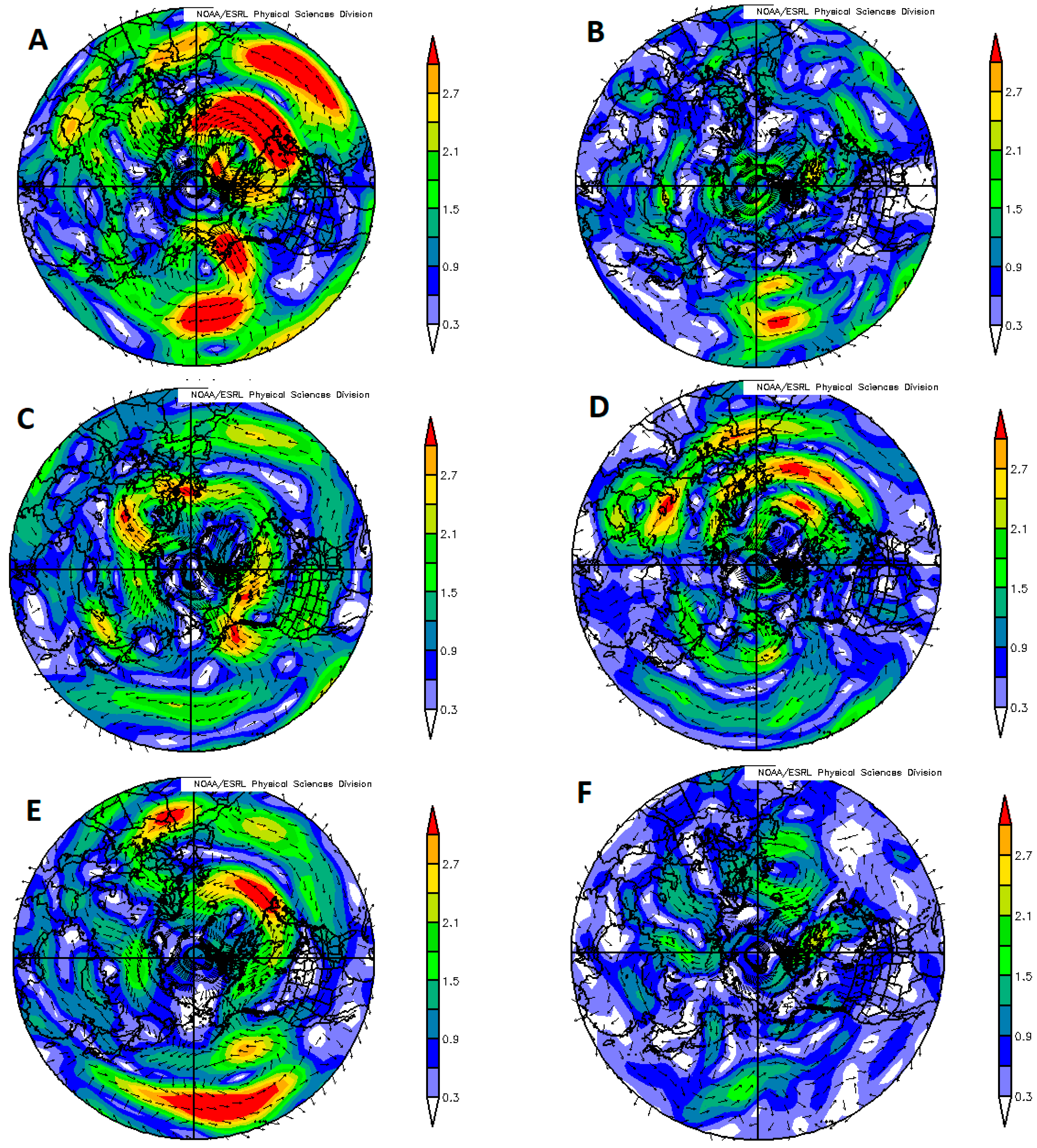
During the mid-twentieth century (Table 1 – P1) the seasonal temperature standard deviations for the temperature anomalies ranged between 0.9 °C in summer to 2.5 °C during the winter (Table 2). Stronger cold season variability is to be expected in the NH. Negative temperature anomalies (−0.1 to −1.0 °C) with respect to the 1957–2017 means were observed for all seasons (Table 2). Only the spring season temperature anomaly was statistically significant at the 95% confidence level. Also, a deficiency in the annual precipitation (53.9 mm/−4.7%) was observed during P1. A shortfall of precipitation (11 and 17% less than the 1957–2017 values) occurred during the summer and fall seasons, respectively, including the vegetation period, which for this region is May-September. The summer season deficiency likely was a cause of adverse agricultural conditions for the region, and eight of the 13 years during P1 showed precipitation deficits (not shown). The middle part of P1 (1961–1964) was the driest, when the negative annual precipitation anomalies ranged from 19% to 25% less than normal [9]. The CV for precipitation was smaller during the summer and fall months (0.34 and 0.28, respectively) including the beginning of the vegetation period (June–July). During the winter season, the CV was 0.41, while the CV was 0.39 during the spring (Table 2). Additionally, Figure 3B shows negative height anomalies over the region during the summer season, consistent with the cool temperature anomalies shown in Table 2. Figure 3A also shows a negative height anomaly over the study region in winter, consistent with an extended Mediterranean storm track (Figure 4A and Figure 5A) and wetter conditions (Table 2).

The beginning of the modern warming (P2) is associated with the transition to a more zonal circulation (Figure 3C,D). The variability of summer season temperature was greater during this period (P2–1.8 °C ). Winter seasons during P2 (1.7 °C) were less variable as those anomalies during P1 (2.5 °C). Negative temperature anomalies were noted for all seasons with respect to the 1957–2017 period (Table 2), and none were significant at the 90% confidence level. With the transition to more zonal conditions as evidenced by weaker 500 hPa height anomalies for P2 (Figure 3C,D) versus P1 (Figure 3A,B), the annual value of precipitation was larger than the base period by 34.8 mm (+6.0%). This reflects the change to positive 500 hPa anomalies at the end of the Mediterranean storm track over the region in winter (Figure 3C) and an extension of this same storm track into the Belgorod region during both seasons (Figure 4C,D and Figure 5C,D). This likely accounts for the higher values for summer season moisture conditions with respect to P1, which are optimal for agriculture. There were only three spring and summers with negative annual average precipitation anomalies, which was the lowest frequency of occurrence of drought years for the entire study period (1957–2017). This is also reflected by low values for CV during these seasons (0.29 and 0.22, respectively—Table 2).

During the period 1981–1997 (P3) (Table 1), there was a further strengthening of zonal circulation types, as shown by the weaker NH 500 hPa height anomalies overall (Figure 3E,F). Within the Belgorod region 500 hPa height anomalies were weakly positive during the winter (Figure 3E) and negative during the summer (Figure 5F). During P3, the seasonal temperature standard deviation ranged from 1.1 °C in the summer to 2.5 °C in the winter season, and these are more comparable to P1. The largest monthly standard deviation for the [4] (1957–2017) epoch was found during the month of February for P3 (4.3 °C), while the minimum value for the monthly temperature standard deviation was noted for July (1.1 °C) (

Table A1. Temperature (°C), precipitation (mm) and their anomalies and CV (2) over periods defined in Table 2 during the current epoch [4] as defined for the study region using the BELF surface data.

Indicator	Months of the Year
	Jan	Feb	Mar	Apr	May	Jun	Jul	Aug	Sep	Oct	Nov	Dec	Year
1881–1980 (base period)
T (°C)	−7.5	−6.8	−1.9	7.5	14.4	17.9	19.6	18.5	12.7	6.1	−0.3	−4.9	6.3
Pre (mm)	40	34	33	39	51	67	65	57	55	44	45	45	575
1957–1969 (P1)
T (°C)	−8.8	−7.9	−3.6	6.2	14.4	17.7	19.6	18.2	12.3	6.0	−0.6	−5.3	5.7
σ	3.9	2.6	2.9	2.2	2.0	1.5	1.5	1.2	1.8	1.9	2.1	3.4	0.8
Pre (mm)	39.2	30.1	32.9	32.5	49.1	48.4	60.2	63.0	49.3	25.3	44.4	46.2	521
CV	0.70	0.56	0.43	0.68	0.55	0.48	0.42	0.56	0.73	0.71	0.55	0.51	0.20
1970–1980 (P2)
T (°C)	−9.6	−7.6	−2.3	7.5	14.1	17.5	18.7	17.6	12.3	5.0	0.1	−4.8	5.7
σ	3.6	3.6	2.5	2.5	2.6	2.2	1.7	2.1	1.8	2.2	2.0	2.8	1.0
Pre (mm)	32.1	31.6	31.7	40.4	46.9	72.6	73.6	63.7	58.5	52.3	54.9	53.4	612
CV	0.63	0.66	0.50	0.58	0.56	0.43	0.48	0.61	0.44	0.41	0.68	0.43	0.20
1981–1997 (P3)
T (°C)	−6.5	−7.1	−2.0	7.1	14.5	17.7	18.7	17.9	12.3	6.1	−1.3	−5.8	6.0
σ	3.7	4.3	3.3	2.5	1.7	2.1	1.1	1.3	1.9	1.2	2.8	2.5	1.1
Pre (mm)	43.1	33.9	26.9	43.3	53.9	68.2	66.0	54.0	55.9	47.7	46.4	38.0	577
CV	0.39	0.30	0.53	0.66	0.51	0.51	0.38	0.54	0.61	0.60	0.72	0.52	0.16
1998–2014 (P4)
T (°C)	−6.4	−5.7	−0.4	8.5	14.8	18.3	20.9	19.5	13.4	6.7	0.4	−4.1	7.2
σ	3.2	3.8	2.8	1.9	2.2	1.8	1.8	1.6	1.3	1.4	2.9	3.3	0.6
Pre (mm)	42.2	36.9	39.8	38.9	52.3	74.5	61.7	54.2	54.1	50.2	39.9	44.0	589
CV	0.44	0.39	0.49	0.53	0.44	0.46	0.57	0.72	0.73	0.56	0.59	0.55	0.18

). Temperature was cooler than the 1957–2017 means for each season except winter, which was similar to the base period mean. During the summer and fall temperature anomalies were cooler but similar to the base period. The cooler summer is consistent with the troughing suggested in Figure 3F. The annual temperature was higher than during P1 or P2, and these warmer temperatures, especially for the winter season, is consistent with global observations [1].

The annual precipitation anomaly for P3 was +2.3 mm (Table 2), which is similar overall to that of the 1957–2017 period, and all seasons were similar to the base period as well. Thus, as may be expected, 50% of the P3 years average annual precipitation anomalies were negative. While many of the months during this period showed similar precipitation amounts or wetter conditions, the months of July and August showed a greater frequency of dry events (Table A1). During these months, the number of years with negative anomalies with respect to the 1881–1980 period was about 70%. The CV was highest during the transition (spring and summer) seasons and smallest for the solstice seasons.

During the modern period (P4 – Table 1), the NH 500 hPa height anomalies were nearly opposite those during P3 for both seasons and the flow became more meridional again (Figure 3G,H). The 500 hPa height anomalies were positive over the Belgorod region for both seasons (Figure 3G,H). The Atlantic Region was characterized by a 25% and 55% increase in the number of blocking events and days according to reference [46], respectively. This agrees with reference [7] which found that the occurrence of blocking doubled from 1970–2010 from 20°–60° W. With these changes in the circulation conditions there were higher average annual temperatures in P4 relative to the 1957–2017 period (+0.9 °C) (e.g., references [7,8,49,50]). A positive mean seasonal temperature anomaly was noted across all seasons of similar magnitude (Table 2). All of the seasonal anomalies were statistically significant at the 95% confidence level, except for winter, which was significant at the 90% confidence level. In addition to the temperature increases for P4 relative to P3, the winter months showed weaker variability (standard deviation 1.9 °C) However, unlike during the previous sub-periods, the lowest values for the monthly standard deviations were noted during the spring (1.0 °C).

Additionally, P4 overall is characterized by precipitation amounts that were 14.0 mm higher annually than the 1957–2017 period. During the summer in P4, the value of the coefficient of variation was 0.28 or only marginally higher than that of P3. The increased precipitation over the region may be related to the increased occurrence of cyclonic flow regime types [6] (not shown). Also, the number of days associated with cold season northwest anticyclone types [6] was acutely reduced for this region. Negative monthly precipitation anomalies in recent years (P4) were related to the sharp increase in the number of stationary anticyclones and blocking occurring over Eastern Europe to Kazakhstan [7,46]. This is reflective of positive height anomalies over the region during the summer season especially (Figure 3H). Lastly, the variance for the precipitation distribution (assuming a gamma-type [30]) for P3 and P4 was slightly larger for each season than for P1 and P2, except for winter, in which the variance was similar.

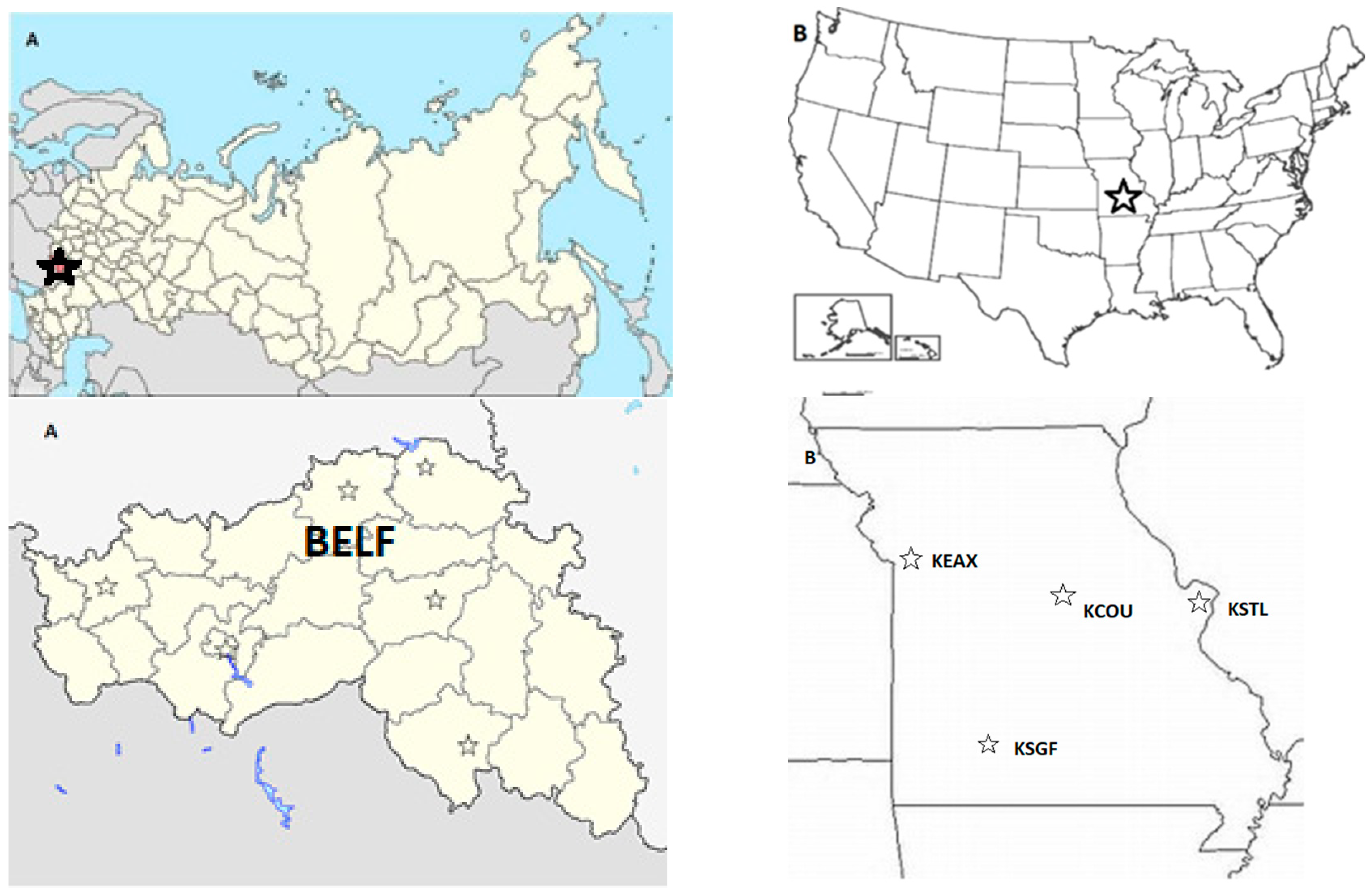
3.2. Climatological Background for the Central USA

If the reference [6] scheme is robust, the climatological results from any other local region governed by the NH flow regimes should be consistent with the regional 500 hPa flow regimes suggested in Figure 3, Figure 4 and Figure 5. In order to answer this question, the climatological data for the Missouri region (Figure 1) in the central United States [17,18,21] are examined in

Table 3. As in Table 2, except for the Columbia, MO station in the USA. Statistically significant values with respect to the base period are marked with a * at the 90% level, and ** at the 95% level.

Indicator	Seasons
	Winter	Spring	Summer	Fall	Year
1957–2017 (base period)
T (°C)	−0.2	12.5	24.3	13.6	12.6
Pa (mm)	150.8	310.5	293.7	251.4	1005.2
1957–1969 (P1)
Ta (°C)	−0.2	−0.3	−0.1	+0.3	−0.1
σ	1.1	1.1	0.6	1.2	0.5
Pa (mm)	−25.2	−40.8	−26.0	−19.0	−113.0
CV	0.33	0.27	0.42	0.36	0.22
1970–1980 (P2)
Ta (°C)	−1.2 **	−0.4	0.0	−0.2	−0.5 *
σ	2.1	1.0	1.2	1.4	0.5
Pa (mm)	−8.3	+12.2	−78.8	−8.1	−82.7
CV	0.46	0.32	0.42	0.32	0.24
1981–1997 (P3)
Ta (°C)	0.0	−0.3	−0.2	−0.6 **	−0.3
σ	1.5	1.4	1.0	0.9	0.7
Pa (mm)	+15.4	+11.6	+42.4	+25.7	+97.3
CV	0.32	0.33	0.44	0.42	0.21
1998–2017 (P4)
Ta (°C)	0.8 **	0.7 **	0.2	0.5 **	0.5 *
σ	2.0	1.4	1.2	1.3	1.0
Pa (mm)	+7.9	+10.0	+24.1	−5.0	+36.0
CV	0.32	0.28	0.35	0.34	0.16

(and

Table A2. As in Table 3, except for the Columbia, MO station in the USA.

Indicator	Months of the Year
	Jan	Feb	Mar	Apr	May	Jun	Jul	Aug	Sep	Oct	Nov	Dec	Year
1957–2017 (base period)
T (°C)	−1.8	0.8	6.6	13.0	18.0	22.9	25.3	24.6	20.1	13.8	6.9	0.6	12.6
Pre (mm)	43	49	76	111	123	103	103	88	100	83	69	57	1005
1957–1969 (P1)
T (°C)	−2.1	0.2	5.2	13.0	18.4	22.8	25.3	24.6	20.3	14.4	7.1	0.5	12.5
σ	2.5	2.2	3.4	1.6	2.2	1.0	1.3	1.2	1.3	2.1	1.9	2.8	0.5
Pre (mm)	39.4	38.7	68.2	92.7	108.7	108.3	114.5	44.7	106.8	81.8	43.9	44.4	892
CV	0.67	0.38	0.41	0.46	0.31	0.67	0.52	0.66	0.63	0.74	0.65	0.46	0.22
1970–1980 (P2)
T (°C)	−3.9	−0.5	6.0	12.7	17.6	22.6	25.6	24.5	20.3	13.6	6.2	0.6	12.1
σ	3.3	3.3	2.2	1.2	1.5	1.4	1.8	1.3	2.2	1.9	2.0	2.2	0.5
Pre (mm)	43.7	42.5	95.3	100.3	127.1	76.1	61.2	77.5	93.2	84.7	65.5	55.8	923
CV	0.70	0.52	0.67	0.48	0.43	0.58	0.63	0.87	0.78	0.48	0.52	0.57	0.24
1981–1997 (P3)
T (°C)	−1.7	1.1	7.0	12.3	17.4	22.7	25.2	24.3	19.5	13.3	6.1	0.1	12.3
σ	2.9	2.8	1.9	1.9	1.9	1.4	1.0	1.7	1.3	1.2	2.0	3.3	0.7
Pre (mm)	41.9	56.5	69.9	117.0	135.2	111.6	115.9	108.7	94.9	73.8	108.4	68.8	1103
CV	0.75	0.75	0.57	0.63	0.52	0.63	0.68	0.54	0.83	0.51	0.62	0.66	0.21
1998–2017 (P4)
T (°C)	−0.7	1.5	7.4	13.7	18.4	23.3	25.2	24.8	20.6	13.9	7.8	1.0	13.1
σ	2.4	3.3	2.9	1.5	1.4	1.3	1.8	1.6	1.8	1.7	2.2	2.7	1.0
Pre (mm)	46.4	54.3	76.3	123.9	120.2	107.7	107.1	102.9	104.4	89.5	52.5	56.0	1041
CV	0.70	0.63	0.52	0.42	0.51	0.39	0.75	0.64	0.67	0.82	0.76	0.68	0.16

).

A comparison of the temperature regimes (Table 2 versus Table 3) shows broad similarities in the annual variability of temperature, or larger standard deviations in the winter season versus the summer season. For the P1 seasons, most of the seasonal temperature anomalies were cooler with respect to the 1957–2017 period (Table 3) but not at standard levels of significance, which is qualitatively similar to that of the southwest Russia Region. Figure 3A,B shows that the 500 hPa height fields in both winter and summer are consistent with cooler conditions over the continental USA as a negative height anomaly (troughing) is observed. This coupled with strong positive anomalies over the Pacific during winter implies more meridional flow regionally. Recall that over the Belgorod Region, there were slight negative (positive) 500 hPa height anomalies in the winter (summer).

Then P2 was the coolest sub-period during the [4] epoch for the central USA (Table 3) as all seasons were the same or cooler than the reference period. The winter season as well as the annual means were significantly cooler than the base period at the 95% confidence level. The strongest negative anomalies of the entire period were noted over the central USA during the winter season (Figure 3C). P3 was also slightly cooler overall for the central USA for all seasons except winter (similar to the base period) but not as cool as P2, with only the fall season being significantly cooler (at the 95% confidence level) than the base period. Figure 3E,F however, suggest weaker meridional or more zonal flow over the central USA and over southwest Russia, with weaker height anomalies overall. During this period the wind anomalies (Figure 4E,F and Figure 5E,F) were also weakest.

Finally, more meridional flow is suggested for the P4 years (Figure 3G,H, Figure 4G,H, and Figure 5G,H) and the mean temperatures for every season were warmer than the 1957–2017 period. These anomalies were significant at the 95% confidence level, except for the summer season (Table 3). Additionally, the increases in winter, spring, and fall season temperatures were statistically significant at the 99% confidence level using the F-test from analysis of variance (ANOVA) when examining the trend from P2 to P4, reflecting the modern warming [1]. The changes in summer temperature were not significant at the 90% confidence level. A similar result was found for the Belgorod Oblast in southwest Russia, except that the temperature change in all seasons was significant at the 95% confidence level or greater.

When examining the precipitation information across the modern epoch [4], the central USA was driest during P1 and generally wetter than the 1889–1980 period for P3 and P4, especially in the spring and summer seasons. The calculated variances for the precipitation distributions using P3 and P4 in each season were 2216.0, 11726.0, 4441.0, and 2537.0, for winter, spring, summer, and fall and these were larger than that of P1 and P2 for each season by a factor of two. This may be a function of the warming conditions prevalent globally during P3, but especially P4.

Examining the distribution of precipitation in P3 and P4 precipitation versus the P1 and P2 period (

Table 4. The distribution of precipitation (mm) by quintile and season for the (a) Belgorod Region, and (b) central USA during P3 and P4 versus P1 and P2.

(a)
% tile	Winter		Spring		Summer		Fall
	P3-P4	P1-P2	P3-P4	P1-P2	P3-P4	P1-P2	P3-P4	P1-P2
20%	90.8	78.2	90.7	85.6	159.2	149.9	106.6	106.1
40%	113.1	110.0	117.2	114.3	177.1	173.1	122.0	121.7
60%	130.9	126.4	140.9	130.7	195.9	196.3	153.0	159.7
80%	144.0	146.9	160.2	158.3	221.4	233.2	183.9	182.3
100%	192.6	200.5	206.2	213.9	292.2	303.5	274.1	274.1
(b)
% tile	Winter		Spring		Summer		Fall
	P3-P4	P1-P2	P3-P4	P1-P2	P3-P4	P1–P2	P3-P4	P1-P2
20%	115.0	86.6	222.8	215.6	199.1	159.3	169.9	164.8
40%	139.4	125.0	273.1	254.3	261.1	202.4	206.8	185.2
60%	175.8	141.7	325.1	288.8	357.9	243.1	247.4	258.1
80%	195.3	161.0	400.8	399.0	432.6	327.4	344.2	329.7
100%	312.4	275.1	520.7	478.0	655.3	487.9	465.1	383.4

) demonstrates that for the winter and summer seasons, the 60th percentile in P3 and P4 was nearly the 80th percentile from the base period. Additionally, the width of the 40–80% bin was 50% larger for the winter season, but more than double the width for the summer season. These results are consistent with reference [51] who found similar results for only the summer season. The distributions for P1and P2 versus P3 and P4 were tested assuming a gamma distribution and using the chi-square goodness of fit test. This analysis demonstrated that the distributions for all seasons were different at the 90% confidence level (except for winter). In the Belgorod region (Table 4), the width of the 40–80% bins were of similar size across all seasons when comparing P3 and P4 to P1 and P2. The same statistical testing for the Belgorod region demonstrated that the distributions were not different at the 90% confidence level. Thus, combined with the variances, the precipitation distributions were similar in this region.

3.3. A Comparison Using the HTC for Both Regions

At the beginning of the 21st century, changes in the Belgorod region atmospheric circulation were associated with an increase in the frequency of quasi-stationary anticyclones, especially during the summer season [7]. This resulted in increasing temperatures during the growing season, but also in the frequency and duration of weather conditions that produce less precipitation [9]. This trend toward more arid conditions especially in the mid-summer (July–August) became stronger during P4 than during the P3 period. The higher variability during P4 also indicated that in some years, there was excess precipitation [8]. For many summer crops (e.g., corn or soybeans), July and August are the most impactful months for reproduction and yield (e.g., reference [51]). Thus, while the annual precipitation was higher during the late 20th century, agriculture has become more vulnerable in the region [9].

The average values of the HTC [31] over the Belgorod Oblast during P1, P2, P3, and P4 was 1.00, 1.27, 1.18, and 1.04, respectively. The CV for the corresponding periods was 0.29, 0.33, 0.22, and 0.29, respectively. Since HTC is derived largely from summer season values, a comparison to Table 2 and Figure 5 for the summer season is most relevant for this discussion. The latter period (P4) shows more similarity to the earliest period (P1) for HTC and precipitation. The temperature was warmer for P4 summers, but the quantities representing variability are similar. Additionally, both P1 and P4 are associated with positive height anomalies in the summer season over the Belgorod Oblast (Figure 3). Optimal conditions for agriculture in the Belgorod region, that is positive temperature and precipitation anomalies, occurred when the flow was becoming more zonal (P2). However, the interannual variability of the HTC was also greater. With the occurrence of meridional circulation during P4, the higher temperature and greater variation of precipitation during the growing season was less optimal for agriculture.

Additionally, the CV was higher generally in the central USA, implying more variable precipitation conditions. This might be expected since the central USA is more continental than southwest Russia (e.g., reference [21]). Lastly, the HTC for the central USA was lower for P1 and P2, 1.60 and 1.51 respectively, reflecting the generally cooler or drier conditions discussed above. During P3 and P4, the HTC was 1.87 and 1.80 for the central USA, and these more favorable growing conditions were partly responsible for higher yields during these sub-periods [51] due to the warmer wetter conditions. Overall, the HTC is higher in the central USA than for the Belgorod Region due primarily to the warmer climate and longer growing seasons [9].

3.4. Discussion: Teleconnection Relationships

The classification scheme of reference [6] for NH flows is consistent with the idea that the NH flow has preferred observed states. This idea is not new (see reference [40] for a discussion of the history). The early work of references [52,53,54] (and others) suggested the NH flow vacillated between two quasi-stable states (zonal versus meridional), but later work suggested that the NH flow possesses multiple stable states, including those that represent blocking (e.g., references [55,56,57,58,59]). More recent work references [60,61,62], have extended this idea to the Atlantic and Pacific Ocean Basin regions separately. Thus, the classification scheme of reference [6] can be considered similar to these studies references [52,53,54,55,56,57,58,59,60,61,62] in that reference [6] suggests 13 recurring states that are grouped into four general classes, two of which are more zonal and two of which are more meridional in nature. As explained in reference [7], many of the sub-types are characterized locally by a trough or ridge, for example, within a particular region.

However, in order to meet a stated goal, that is the comparison of composite types of reference [6] to teleconnection indexes, it is useful to compare to the results of other studies (e.g., reference [62]). That study [62], used the finite element, bounded-variation, vector autoregressive factor method (FEM-BV-VARX) in order to describe the structure of major teleconnection patterns and relate these to the teleconnection indexes in several re-analysis products including the NCEP/NCAR reanalyses used here. A strict comparison here will be difficult to make since reference [62] uses the entire 1948–2014 period and displays composites that include all months.

Nevertheless, some comments can be made here and will be discussed below. Since the ECM of [6] were originally subjectively identified on the basis of the amplitude of the NH flow and the number and location of strong ridge trough couplets in the NH wide flow, it is possible, for example, to have positive NAO events of Type 2, but also of Type 3. These two situations will differ based on the existence of strong trough/ridge couplets occurring elsewhere across the NH and, generally, the amplitude of the flow. Thus, the ECM of [6] may not necessarily be dynamically distinct (at least locally) and full correspondence between teleconnections and the [6] flow types will not be possible. Further study based on the results found here would be needed to determine whether the [6] ECM were dynamically distinct. Also, work such as reference [63] demonstrate the challenges associated with using clustering techniques to confirm or identify the existence of dynamically stable flow regime types in the NH flow.

Here, a seasonal analysis of the mean daily teleconnection indexes was carried out (

Table 5. The prominent teleconnection indexes for the 1957–2017 epochs [4] in Table 2. The indexes are the North Atlantic Oscillation (NAO), Pacific North American (PNA), and the Arctic Oscillation (AO). The indexes are shown for all seasons W/S/S/F.

Years	NAO	PNA	AO
1957–1969	−0.53/−0.18/−0.15/+0.05	−0.13/−0.31/+0.42/+0.16	−0.91/−0.12/−0.26/−0.23
1970–1980	−0.19/−0.13/+0.20/+0.16	−0.07/+0.03/−0.32/+0.11	−0.46/−0.17/−0.03/+0.08
1981–1997	+0.46/+0.31/+0.16/−0.10	+0.29/+0.27/+0.03/−0.33	+0.11/+0.09/+0.05/+0.04
1998–2017	+0.37/+0.09/−0.54/−0.13	+0.38/−0.05/+0.23/+0.23	−0.14/+0.17/−0.12/−0.00

). The correlation between the AO and NAO Index time series from 1957–2017 for all seasons ranged between 0.54–0.77 which is significant at the 99% confidence level. Similar correlations were noted for each sub-period (P1–P4), which in some cases were even higher. With the PNA Index time series, the correlations to the AO were negative (between −0.15 to −0.48), but statistically significant for all seasons except the winter for the entire period (1957–2017). These correlations are significant at the 95% confidence level. A similar result was obtained for P1, P2, P3. For P4, the negative AO-PNA correlations were not statistically significant at the 90% confidence level. However, the correlations for the subperiods should be viewed more cautiously since the sample sizes are much smaller. There were no significant correlations between the NAO and PNA index time series for the entire period, and the sign was different by season and subperiod. This is consistent with the results of reference [64].

The P1 years were characterized as negative for both the decadal modes of the PDO and the NAO epochs as in Section 2. The AO is negative for a meridional NH flow regime, while a positive AO is associated with a zonal NH flow regime. For P1, the AO was strongly negative for all seasons which is consistent with Figure 3A,B. Cooler conditions over the southeast USA including the Missouri region are consistent with references [47,48]. The NAO index shows negative values (Table 5) in the winter and summer season, and the 500 hPa height anomalies are consistent with negative NAO (ridging in the Atlantic).

The winter season 5000 hPa anomalies (Figure 3A) resemble `state ` 1 (positive height) anomaly over Greenland – negative anomalies over the mid-latitude Atlantic) for the NAO and ‘state 2’ (positive height anomaly over the polar region, negative height anomalies in the mid-latitudes) for the AO from reference [62]. The summer season is similar, but weaker. The PNA index was negative in the winter and positive in the summer (Table 5) with the 500 hPa height anomalies reversing sign in the Gulf of Alaska region. The winter (summer) season 500 hPa anomalies also resemble the ‘state 1’ (‘state 2’) PNA in reference [62], or a positive (negative) height anomaly over the Bering Sea Region. 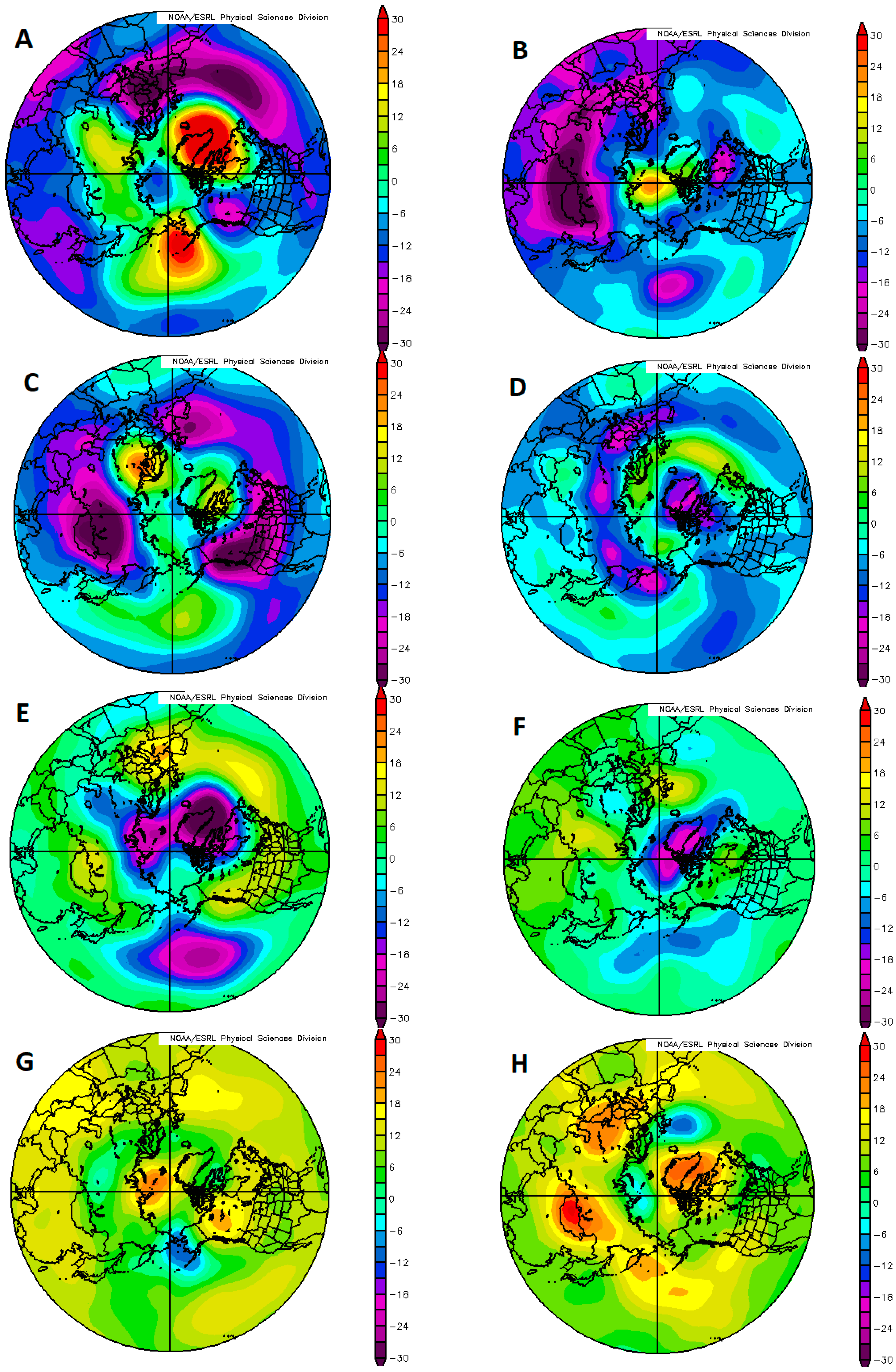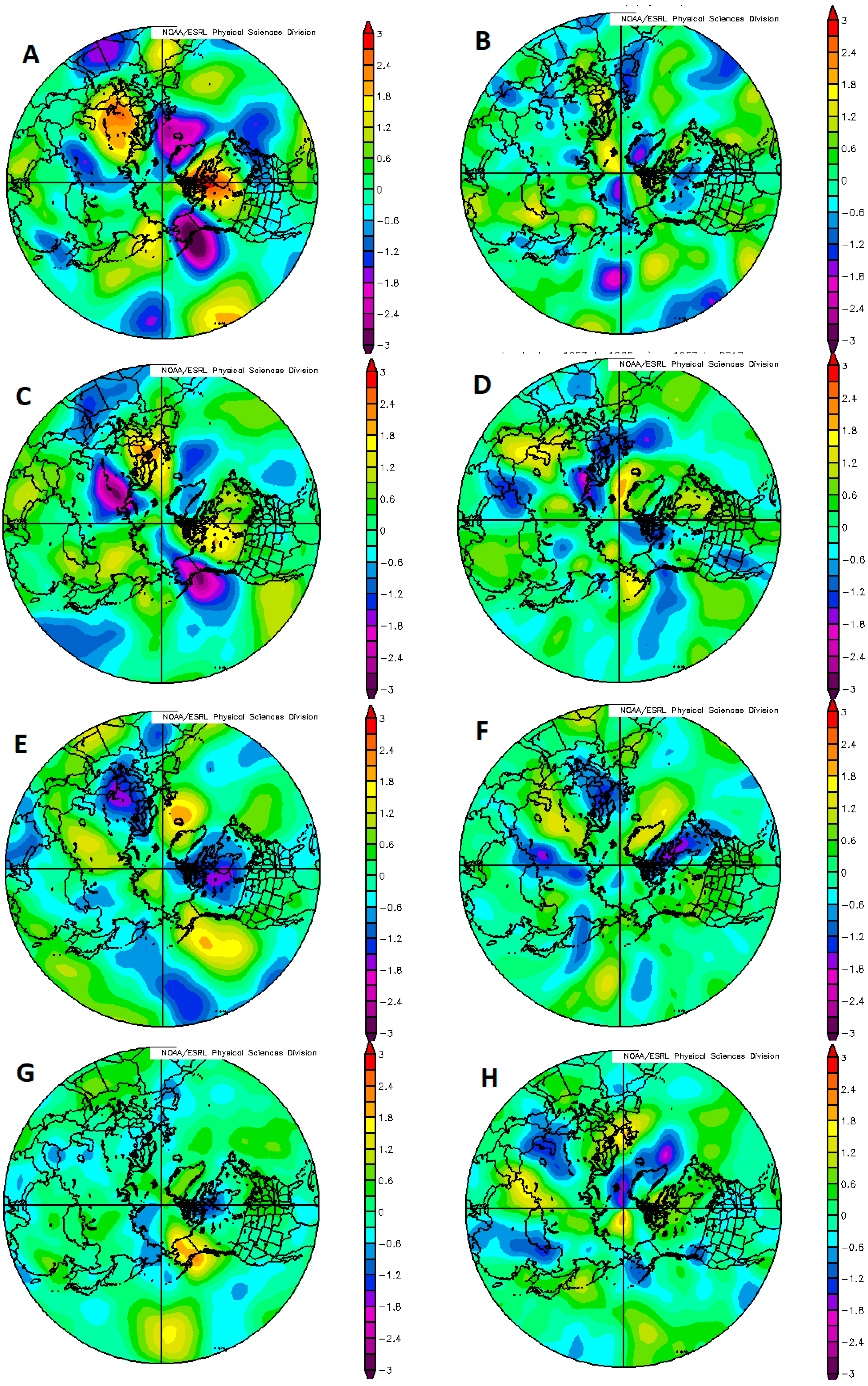Examining the 300 hPa meridional wind anomalies (Figure 4A,B) and vector wind anomalies (Figure 5A,B) also suggest strong meriodional flow, which was the strongest for the entire epoch (1957–2017).

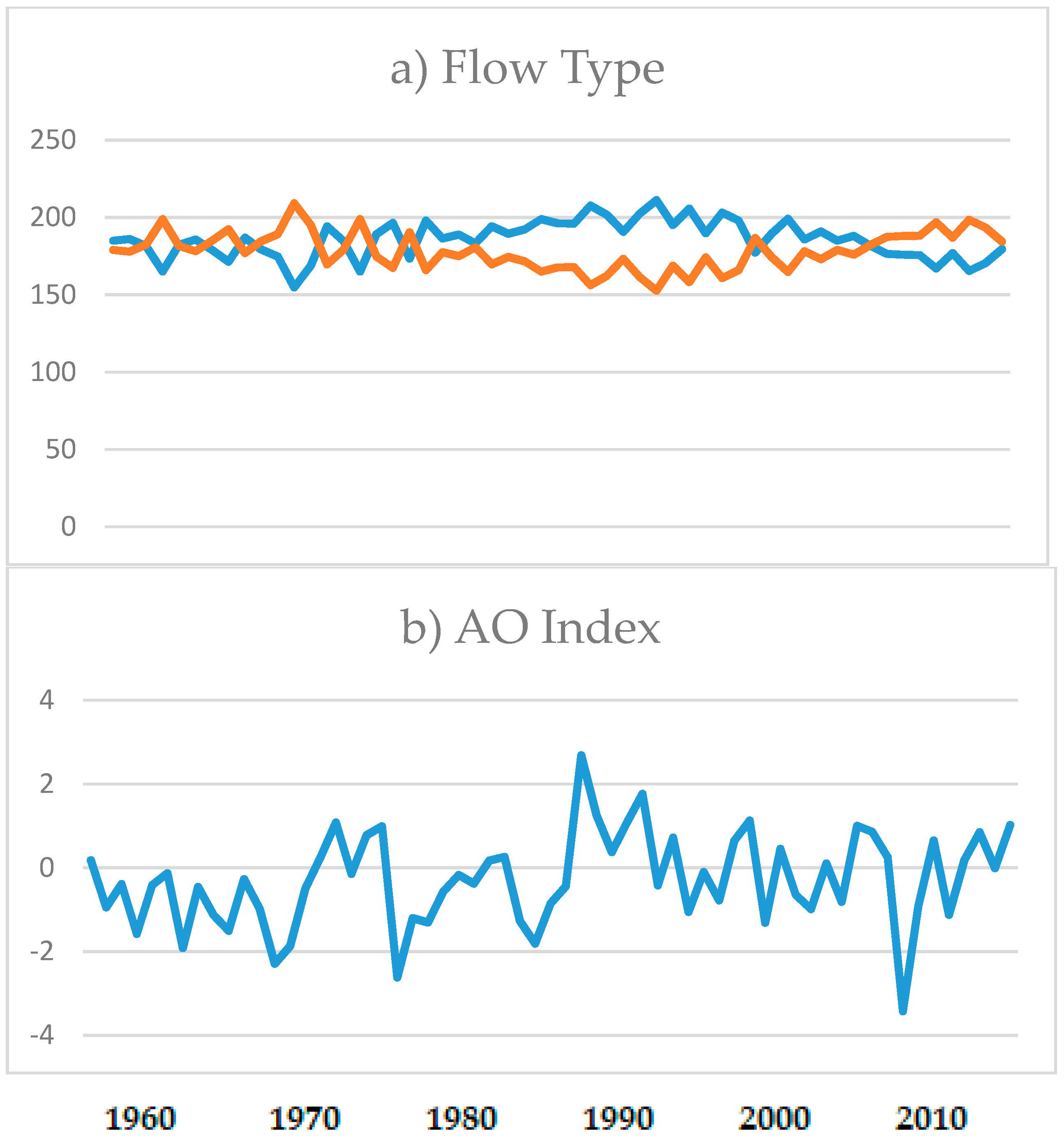
The P1 time period was associated with about 12 more days (6%) of high amplitude Type 3 and Type 4 flows on an annual basis in both regions. For the entire 1957–2017 period (Figure 6), there was eight fewer days of Type 3 and Type 4 flows per year in the NH. However, the long-term trend in the occurrence of zonal versus meridional flows over the entire period is consistent with the results of, for example reference [62] (see their Figure 10) and with the indexes in Table 5. The standard deviation was 12 and 10 days for the 1957–2017 period and P1, respectively. Treating the occurrence of Type 3 and Type 4 flow as a Baysean process (since the alternative is Type 1 and Type 2 flow) (e.g., references [17,28]), the observed occurrence of a more meridional flow regime was tested against the random probability for the occurrence of meridional flow. For the entire period and P1, the result was not statistically significant.

The P2 years were characterized by the transition of the decadal modes for the NAO (1972) and the PDO (1976) to their positive phases. Again, all seasons in the southwest Russia region were cooler than that of the reference period. The 500 hPa height field (Figure 3C,D) for P2 is similar to that of P1, but there were stronger negative anomalies over the USA in the winter season. Additionally, Figure 4C,D and Figure 5C,D support the results of reference [4], who suggested that conditions became more zonal during this period. The AO (Table 5) was generally negative across all seasons but smaller than for P1, supporting a more zonal NH epoch that P1 (see Figure 3C,D, Figure 4C,D and Figure 5C,D). The mean daily NAO was negative in the winter and positive in the summer over the Atlantic Region, while the PNA index was negative in both the summer and winter seasons over the Pacific. The winter season NAO and PNA still resembles the ‘state 1’ (and ‘state 2’ of the AO’) of reference [62] for both regions (see also Table 5). Also, Table 1 shows that the proportion of zonal flow days increased for both regions, resulting in a similar number of Type 3 and 4 flows versus more zonal Type 1 and 2 flow days per year as for the entire period (1957–2017). The standard deviation for the P2 period was 10 days.

During P3, the decadal modes of the PDO and NAO were both in their positive phase throughout this period, although the NAO transitioned to the negative phase in 1996. The PDO transitioned to the negative phase in 1998. An examination of the AO supports (Table 5) the conclusion that this epoch was the most zonal across the NH as the index were now weakly positive during this epoch (see Figure 3E,F, Figure 4E,F and Figure 5E,F). Table 1 also shows that the number of zonal flow days increased in both study regions for this time period such that there were 50, and 14 more zonal flow Type 1 and 2 flow days (per year) observed in the southwest Russia and central USA regions, respectively. The standard deviation for P3 was eight days. Using the same Baysean testing for P3 demonstrated that the occurrence of more zonal flow types for this period was statistically significant at the 90% confidence level. In Figure 6a, there were clearly more zonal flow days over the entire NH, and this corresponds to the AO being positive (Table 5). The same analysis as in Figure 6 was carried out for each region, and this test showed similar results. The daily NAO and PNA indexes were positive across almost all seasons during this epoch (Table 5). Figure 3E,F now resemble ‘state 2’ for both the PNA and NAO regimes (and ‘state 1’ of the AO regime) shown in reference [62], and this resemblance is stronger during the winter season. For the NAO and AO, these states are characterized by negative height anomalies over Greenland and the Arctic, and positive height anomalies in the mid-latitudes.

Then during P4, the decadal modes of the PDO and NAO have been predominantly negative through this period as in P1, though the NAO entered a new positive phase starting in 2011. In Table 5, the AO returned to negative values for most seasons, except for spring, supporting a return to more meridional flow generally. The daily NAO and PNA indexes were positive across all seasons. Table 1 demonstrates also the return to the more frequent occurrence of meridional (Type 3 and Type 4) flows in both regions during P4. In the southwest Russia region, the number zonal flow regime days per year are similar to the number of meridional flow days. In the central USA region, there were about 10 more meridional flow days per year during P4. The standard deviation was nine days for P4. This result is not significantly different from that of the entire period or a random process. Figure 3G,H also show a return to ‘state’ 2 conditions for the AO, as was the case for P1.

Thus, three points can be made overall when summing up the results of this investigation. The first is that the climatologies of the Belgorod Region and the central USA region examined here are consistent with the local 500 hPa height anomalies shown in Figure 3 for both the summer and winter seasons. In the Belgorod Region, the winter and spring season warm throughout the period, while in the central USA P1 and P4 were warmer that P2 and P3 with P4 being the warmest relative to their base periods. In the Belgorod region, the warming trend of the late 20th and early 21st century is statistically significant across all seasons. In the central USA, the warming trend during the period was significant for each season except for the summer. The results are also consistent with a warming climate overall [1,62]. The work of reference [65] (and references therein) also show that mean annual precipitation has increased over the USA overall since the middle 20th century. The results in the Belgorod Region are consistent with the increase in blocking across the region, especially into the early 21st century [46,66,67].

Secondly, the daily mean values of the NAO (and PNA) index shows some (only weak) correspondence with the temperature and precipitation trends from P1 to P4 (see Table 2, Table 3, and Table 5) in both regions. This is consistent with studies from many authors for the central USA (see reference [64] and references therein). This also supports the study of reference [19] that showed stronger correspondence with the NAO and extreme temperature anomalies in the Belgorod Region. Correlating the time series of seasonal temperature and precipitation with the NAO resulted in a correlation coefficient of 0.49 and 0.60 (significant at the 95% confidence level or higher) in the central USA and Belgorod region during winter, respectively. Only the summer season temperature (−0.30) and precipitation (−0.36) in the central USA was negatively correlated with the NAO at the 95% confidence level. None of the mean daily PNA index values correlated at standard levels of significance with temperature and precipitation, although strong positive values were noted in winter. The tendency for the more frequent annual mean occurrence of meridional flow regime types (Type 3 and Type 4) were consistent with the changes in the NAO index with time, especially in the southwest Russia region. These time-series correlated at −0.40 and −0.30 (significant at the 95% and 90% confidence level) for both southwest Russia and the central USA respectively. For the PNA index there was a positive relationship between the more frequent occurrence of Type 3 and Type 4 flows in the central USA only, but this correlation was not statistically significant and reached standard levels.

There is a better comparison of central USA temperature with the AO, which is consistent with reference [47,48], and a better comparison of the AO with the temperature anomalies of both regions for P1 to P3 (generally cooler in P1 with a negative AO and warmer in P3 with positive AO). During P4, the temperature of both regions is warmer in spite of more negative AO. For the time series of mean seasonal AO, positive correlations were noted at the 90% confidence level (>0.22) for winter, spring, and fall in both regions, however, in winter and spring the correlations were significant at the 95% confidence level (Belgorod–winter 0.48, spring 0.28, central USA 0.46 winter, 0.35 spring). Only the precipitation correlated negatively (−0.34) in the winter season in the Belgorod region at the 95% confidence level. Additionally, the more frequent annual mean occurrence of meridional type flow regimes (Type 3 and Type 4) was consistent with the behavior of the AO index over time for both regions.

Lastly, it is suggested here that the occurrence of the NH meridional flow types [6] are increasing or more persistent when the decadal mode of the PDO and NAO are concurrently in their negative phases (P1 and P2), while more zonal flow regime types are dominant during the concurrent positive phases of the PDO and NAO (P3). The values and trends for the mean daily AO (Table 5) and annual mean occurrence of Type 3 and Type 4 flows were consistent as well with the discussion regarding meridional versus zonal flow here. As shown above, the tendency for more zonal flow conditions was statistically significant during the P3 time period (positive PDO and NAO) if the occurrence of zonal flow versus meridional flow is treated as a Baysean process. These results are also consistent with trends in the NH climatology of blocking during a similar time period as blocking was at a minimum during P3 and higher during P4 [46]. Other studies also show an increase in blocking globally, albeit in more limited regions or seasons [10,66,67] than reference [46]. Additionally, there are anecdotal observations available that weather and climate conditions of the first part of the 21st century were similar to those of the middle part of the 20th century in the central USA. While this would support the conclusions made here, additional and more detailed studies would be needed to confirm this conjecture.

4. Conclusions

Using surface data provided by the Belgorodskoye-Feninio and Columbia, MO weather stations, the climatological character of the southwest Russia region studied by references [7,8,9], and the central USA by references [17,18,19], and reference [51] for the growing season was expanded to incorporate the entire year. Using the classification scheme of reference [6], the NH flow can be binned into 13 ECMs. This scheme was modified by reference [3] and described in greater detail in references [3,7,8]. These 13 ECMs can fit more broadly into four NH-wide circulation groups (Types 1–4), two of which are more zonal type flows and two of which are more meridional flows. The [6] classification scheme for NH flow regimes is similar conceptually to many studies which argue that the NH flow can be classified into either two basins of attraction (e.g., reference [52]) or multiple stable states (e.g., reference [55]).

Furthermore, reference [4] showed using the reference [6] classification scheme that a prolonged meridional circulation epoch that began in 1957 continues up to the present day. Here, we demonstrate that within this epoch there are four sub-periods that can be described by variations in the predominance of more zonal versus more meridional flows by examining 500 hPa height and 300 hPa winds using the NCEP/NCAR re-analyses. These sub-periods are marked by the significant variation of the climatological character of the temperature and precipitation regimes that dominated both study regions. The temperature and precipitation character was compared to the 1957–2017 climatological record.

The temperature has become gradually warmer over both regions (significantly over all seasons), while the annual precipitation was the least during P1. This period was marked by more meridional NH circulation patterns. In the central USA region, the temperature was coldest during P2. In southwest Russia, the annual precipitation and HTC was greatest during P2. The HTC combines both temperature and precipitation characteristics during the growing season. A higher value for HTC is associated with potentially better growing conditions. This period (P2) was associated with a trend toward more zonal flow over the region, a condition generally associated with a stronger Mediterranean storm track. The latter sub-periods (1981–1997, and 1998–2017) showed increasing temperature in both regions. The HTC decreased during both periods, suggesting greater evaporation during the growing season in southwest Russia. This situation is less favorable to regional agriculture. The warmer temperatures have been associated with the increased occurrence of blocking in all seasons.

Finally, in order to test the climatological robustness of the reference [6] classification scheme, the climatological character of the central USA was compared over the same sub-periods of the 1957–2017 circulation epoch suggested by reference [4] as well as with various teleconnection indexes. The results for both the Belgorod Region and central USA were consistent with the regional flow regimes suggested by the 500 hPa height and 300 hPa wind anomalies for these sub-periods. Also, the decadal variation in the strength of the NH meridional flow suggested by the reference [6] ECMs were consistent with the decadal variability of the mean daily AO presented here. The mean daily NAO (and PNA) show some (only weakly) correspondence to the local seasonal temperature, while the AO correlated significantly in all seasons but summer. Additionally, the results of this study demonstrated that long-term trends and variations in the reference [6] classification scheme also corresponded with the occurrence of concurrent positive or negative phases of the PDO and the decadal mode of the NAO. The results found here were also consistent with long-term trends in the occurrence and intensity of NH blocking, and the winter season temperatures of both regions increased significantly from P1 to P4 in accord with changes in global temperature [1,65]. These results will provide more information for seasonal range forecasts being produced routinely for Missouri in the central USA, and also in the Belgorod Region. Finally, additional study will be carried out to test the dynamic significance of the reference [6] flow types or ECM.

References

1. Intergovernmental Panel on Climate Change (IPCC). Climate Change 2013: The Physical Scientific Basis. 2013. Available online: http://www.ipcc.ch (accessed on 7 August 2018).
2. Kononova, N.K. Fluctuations of Atmospheric Circulation in the XX—Beginning of the XXI Centuries. 2009. Available online: http://www.atmospheric-circulation.ru (accessed on 12 December 2018).
3. Kononova, N.K. Warming or climate variations. In Proceedings of the Collection of Scientific Works of the XIV Congress of the Russian Geographical Society, Saint Petersburg, Russia, 11–14 December 2010; Volume 1, pp. 44–48. [Google Scholar]
4. Kononova, N.K. Features of the atmospheric circulation of the Northern hemisphere at the end of XX—Beginning of XXI century and their reflection in the climate. Complex Syst. 2014, 2, 11–35. [Google Scholar]
5. Climate Research Unit: Data (2018). Available online: http://www.cru.uea.ac.uk/data/temperature/ (accessed on 11 December 2018).
6. Dzerdzeevskii, B.L. Circulation Mechanisms in the Atmosphere of the Northern Hemisphere in the XX Century/Proceedings of the Meteorological Studies. Master’s Thesis, Publishing House of Institute of Geography, USSR Academy of Sciences and Interagency Geophysical Committee at the Presidium of the USSR Academy of Sciences, Moskva, Russia, 1968; 240p. [Google Scholar]
7. Lebedeva, M.G.; Krymskaya, O.V.; Lupo, A.R.; Chendev, Y.G.; Petin, A.N.; Solovyev, A.B. Trends in Summer Season Climate for Eastern Europe and Southern Russia in the Early 21st Century. Adv. Meteorol. 2016, 2016, 5035086. [Google Scholar] [CrossRef]
8. Lebedeva, M.G.; Krymskaya, O.V.; Chendev, Y.G. Agroclimatic resources of the Belgorod oblast at the beginning of XXI century. Sci. Technol. APC 2016, 30, 71–75. [Google Scholar]
9. Lebedeva, M.G.; Lupo, A.R.; Henson, C.B.; Solovyov, A.B.; Chendev, Y.G.; Market, P.S. A Comparison of Bioclimatic potential of Two Global Regions during the Late 20th Century and Early 21st Century. Int. J. Biometeorol. 2018, 62, 609–620. [Google Scholar] [CrossRef] [PubMed]
10. Mokhov, I.I.; Akperov, M.G.; Prokofyeva, M.A.; Timazhev, A.V.; Lupo, A.R.; Le Treut, H. Blockings in the Northern Hemisphere and Euro-Atlantic region: Estimates of changes from reanalyses data and model simulations. Doklady 2012, 449, 430–433. [Google Scholar] [CrossRef]
11. Woollings, T.; Barriopedro Cepero, D.; Methven, J.; Son, S.-W.; Martius, O.; Harvey, B.; Sillmann, J.; Lupo, A.R.; Seneviratne, S. Blocking and its response to climate change. Curr. Clim. Chang. Rep. 2018, 4, 287–300. [Google Scholar] [CrossRef]
12. Medhaug, I.; Stople, M.B.; Fischer, E.M.; Knutti, R. Reconciling controversies about the ‘global warming hiatus’. Nature 2017, 545, 41–47. [Google Scholar] [CrossRef] [PubMed]
13. Zhao, J.; Zhan, R.; Wang, Y. Global warming hiatus contributed to the increased occurrence of intense tropical cyclones in the coastal regions along East Asia. Sci. Rep. 2018, 8, 6023. [Google Scholar] [CrossRef] [PubMed] [Green Version]
14. Blunden, J.; Arndt, D.S. (Eds.) State of the Climate in 2016. Bull. Am. Meteorol. Soc. 2017, 98, Si-S277. [Google Scholar] [CrossRef]
15. Hu, S.; Federov, A.V. The extreme El Nino of 2015-2016 and the end of the global warming hiatus. Geophys. Res. Lett. 2017, 44, 3816–3824. [Google Scholar] [CrossRef]
16. Mokhov, I.I.; Khon, V.C.; Timazhev, A.V.; Chernokulsky, A.V.; Semenov, V.A. Hydrological Anomalies and Trends in the Amur River Basin Due to Climate Changes. In Extreme Floods in the Amur River Basin: Causes, Forecasts, and Recommendations, Roshydromet, Earth Climate Theory Studies; WMO: Geneva, Switzerland, 2014; pp. 81–121. [Google Scholar]
17. Birk, K.; Lupo, A.R.; Guinan, P.E.; Barbieri, C.E. The interannual variability of midwestern temperatures and precipitation as related to the ENSO and PDO. Atmofera 2010, 23, 95–128. [Google Scholar]
18. UMC Climate Change Group Long Range Forecasts. 2018. Available online: http://lrforecasts.missouriepscor.org/about (accessed on 19 October 2018).
19. Newberry, R.G.; Lupo, A.R.; Jensen, A.D.; Rodriges-Zalipynis, R.A. An Analysis of the Spring-to-Summer Transition in the West Central Plains for Application to Long Range Forecasting. Atmos. Clim. Sci. 2018, 6, 375–393. [Google Scholar] [CrossRef]
20. Lebedeva, M.G.; Krymskaya, O.V.; Chendev, Y.G. Changes in the conditions of atmospheric circulation and regional climate characteristics at the turn of XX-XXI centuries. Bull. Belgorod State Univ. Nat. Sci. 2018, 40, 157–163. [Google Scholar]
21. Nunes, M.J.; Lupo, A.R.; Lebedeva, M.G.; Chendev, Y.G.; Solovyev, A.B. The occurrence of extreme monthly temperatures and precipitation in two global regions. Pap. Appl. Geogr. 2017, 3, 143–156. [Google Scholar] [CrossRef]
22. Rohli, R.V.; Vega, A.J. Climatology, 4th ed.; Jones and Bartlett: Burlington, MA, USA, 2017; 466p, ISBN1 0-7637-3828-X. ISBN2 978-0-7637-3828-0. [Google Scholar]
23. Chen, D.; Chen, H.W. Using the Koeppen classification to quantify climate variation and change: An example for 1901–2010. Environ. Dev. 2013, 6, 69–79. [Google Scholar] [CrossRef]
24. Lupo, A.R.; Mokhov, I.I.; Chendev, Y.G.; Lebedeva, M.G.; Akperov, M.G.; Hubbart, J.A. Studying summer seasons drought in Western Russia. Adv. Meteorol. 2014, 2014, 942027. [Google Scholar] [CrossRef]
25. Kalnay, E.; Kanamitsu, M.; Kistler, R.; Collins, W.; Deaven, D.; Gandin, L.; Iredell, M.; Saha, S.; White, G.; Woollen, J.; et al. The NCEP/NCAR 40-year reanalysis project. Bull. Am. Meteorol. Soc. 1996, 77, 437–471. [Google Scholar] [CrossRef]
26. Materials of the Belgorod Center for Hydrometeorology and Environmental Monitoring for 1900–2016; Belgorod Stat National Research University: Belgorod, Russia, 2016. (In Russian)
27. Scientific-Applied Handbook of the USSR Climate; Series 3, Long-Term Data, Parts 1–6; Gidrometeoizdat: Leningrad, Russia, 1990; Volume 28, 366p.
28. Neter, J.; Wasserman, W.; Whitmore, G.A. Applied Statistics, 3rd ed.; Allyn and Bacon Press: Boston, MA, USA, 1988; 2029p. [Google Scholar]
29. Lupo, A.R.; Kelsey, E.P.; McCoy, E.A.; Halcomb, C.E.; Aldrich, E.; Allen, S.A.; Akyuz, F.A.; Skellenger, S.; Bieger, D.G.; Wise, E.; et al. The presentation of temperature information in television broadcasts: What is normal? Nat. Weather Dig. 2003, 27, 53–58. [Google Scholar]
30. Lupo, A.R.; Hagen, T.; Glisan, J.; Aldrich, E.A.; Guinan, P.E.; Market, P.S. The presentation of precipitation information in television broadcasts: What is normal? Nat. Weather Dig. 2008, 32, 2. [Google Scholar]
31. Selyaninov, G.T. On agricultural climate valuation. Proc. Agric. Meteorol. 1928, 20, 165–177. (In Russian) [Google Scholar]
32. Gustokashina, N.N.; Maksutova, E.V. The tendencies of the climatic fridiy change in steppe and forest-steppe of the Baikal region. Geogr. Nat. Res. 2006, 4, 76–81. (In Russian) [Google Scholar]
33. Strashnaya, A.I.; Maksimenkova, T.A.; Chub, O.V. Agrometeorological specifics of the 2010 drought in Russia in comparison with past droughts. Works Russ. Hydro-Meteorol. Cent. 2011, 345, 171–188. (In Russian) [Google Scholar]
34. Matveev, S.M.; Chendev, Y.G.; Lupo, A.R.; Hubbart, J.A.; Timashuk, D.A. Climatic changes in the East-European forest-steppe and their effects on scotch pine annual rings increment. Pure Appl. Geophys. 2016, 174, 427–443. [Google Scholar] [CrossRef]
35. Center for Ocean and Atmosphere Prediction Studies (COAPS). Available online: http://coaps.fsu.edu (accessed on 15 November 2018).
36. Wallace, J.M.; Gutzler, D.S. Teleconnections in the geopotential height field during the Northern Hemisphere winter. Mon. Weather Rev. 1981, 109, 784–812. [Google Scholar] [CrossRef]
37. Feldstein, S.B. The dynamics of NAO teleconnection pattern growth and decay. Q. J. R. Meteorol. Soc. 2003, 129, 901–924. [Google Scholar] [CrossRef] [Green Version]
38. Luo, D.; Lupo, A.R.; Wan, H. Dynamics of eddy-driven low-frequency dipole modes. Part I: A simple model of North Atlantic Oscillations. J. Atmos. Sci. 2007, 64, 3–28. [Google Scholar] [CrossRef]
39. Luo, D.; Gong, T.; Lupo, A.R. Dynamics of eddy-driven low-frequency dipole modes. Part II: Free mode characteristics of NAO and diagnostic study. J. Atmos. Sci. 2007, 64, 29–51. [Google Scholar] [CrossRef]
40. Jensen, A.D.; Lupo, A.R.; Mokhov, I.I.; Akperov, M.G.; Sun, F. The dynamic character of Northern Hemisphere flow regimes in a near term climate change projection. Atmosphere 2018, 9, 27. [Google Scholar] [CrossRef]
41. Da Costa, E.D.; de Verde, A.C. The 7.7-year North Atlantic Oscillation. Quart. J. R. Meteorol. Soc. 2002, 128, 797–818. [Google Scholar] [CrossRef]
42. Mokhov, I.I.; Smirnov, D.A. El Nino–Southern Oscillation drives North Atlantic Oscillation as revealed with non-linear techniques from climatic indicies. Geophys. Res. Lett. 2006, 33, 3708–3711. [Google Scholar] [CrossRef]
43. Wang, Y.-H.; Magnusdottir, G.; Stern, H.; Tian, X.; Yu, Y. Decadal variability of the NAO: Introducing an augmented NAO index. Geophys. Res. Lett. 2012, 39, L21702. [Google Scholar] [CrossRef]
44. Woollings, T.; Franzke, C.; Hodson, D.L.R.; Dong, B.; Barnes, E.A.; Raible, C.C.; Pinto, J.G. Contrasting interannual and multidecadal NAO variability. Clim. Dyn. 2015, 45, 539–556. [Google Scholar] [CrossRef]
45. Climate Prediction Center. Monthly NAO Index. Available online: http://www.cpc.ncep.noaa.gov/products/precip/CWlink/pna/month_nao_index.shtml (accessed on 13 December 2018).
46. Lupo, A.R.; Jensen, A.D.; Mokhov, I.I.; Timazhev, A.V.; Eichler, T.E.; Efe, B. Changes in Global Blocking Character During the First Part of the 21st Century. Atmosphere 2018. Submitted. [Google Scholar]
47. Higgins, R.W.; Leetmaa, A.; Xue, Y.; Barnston, A. Dominant factors influencing the seasonal predictability of U.S. precipitation and surface air temperature. J. Clim. 2000, 13, 3994–4017. [Google Scholar] [CrossRef]
48. Higgins, R.W.; Leetmaa, A.; Kousky, V.E. Relationships between climate variability and winter temperature extremes in the United States. J. Clim. 2002, 15, 1555–1572. [Google Scholar] [CrossRef]
49. Сhendev, Y.G.; Lupo, A.R.; Petin, A.N.; Lebedeva, M.G. Influence of long- and short-term climatic changes on chernozem soils: Central Chernozem Region of Russia. Pap. Appl. Geogr. 2013, 36, 156–164. [Google Scholar]
50. Petin, A.N.; Lebedeva, M.G.; Krymskaya, O.V.; Chendev, Y.G.; Kornilov, A.G.; Lupo, A.R. Regional manifestations of changes in atmospheric circulation in Central Black Earth Region (By the Example of Belgorod Region). Adv. Environ. Biol. 2014, 8, 544–547. [Google Scholar]
51. Henson, C.B.; Lupo, A.R.; Market, P.S.; Guinan, P.E. ENSO and PDO-related climate variability impacts on Midwestern United States crop yields. Int. J. Biol. 2017, 61, 857–867. [Google Scholar] [CrossRef] [PubMed]
52. Lorenz, E.N. Deterministic, non-periodic flow. J. Atmos. Sci. 1963, 20, 130–141. [Google Scholar] [CrossRef]
53. Hansen, A.R. Observational characteristics of atmospheric planetary waves with bimodal amplitude distributions. Adv. Geophys. 1986, 29, 101–134. [Google Scholar]
54. Sutera, A. Probability density distribution of large-scale atmospheric flow. Adv. Geophys. 1986, 29, 227–250. [Google Scholar]
55. Charney, J.G.; DeVore, J.G. Multiple flow equilibria in the atmosphere and blocking. J. Atmos. Sci. 1979, 36, 1205–1216. [Google Scholar] [CrossRef]
56. Mo, K.; Ghil, M. Cluster analysis of multiple planetary flow regimes. J. Geophys. Res. 1988, 93, 10927–10952. [Google Scholar] [CrossRef]
57. Molteni, F.; Tibaldi, S.; Palmer, T.N. Regimes in the wintertime circulation over northern extratropics. I: Observational evidence. Q. J. R. Meteorol. Soc. 1990, 116, 31–67. [Google Scholar] [CrossRef]
58. Smyth, P.; Ide, K.; Ghil, M. Multiple Regimes in Northern Hemisphere Height Fields via Mixture Model Clustering. J. Atmos. Sci. 1999, 56, 3704–3723. [Google Scholar] [CrossRef]
59. Franzke, C.; Woollings, T.; Martius, O. Persistent circulation regimes and preferred regime transitions in the North Atlantic. J. Atmos. Sci. 2011, 68, 2809–2825. [Google Scholar] [CrossRef]
60. Michel, C.; Rivière, G. The link between Rossby wave breakings and weather regime transitions. J. Atmos. Sci. 2011, 68, 1730–1748. [Google Scholar] [CrossRef]
61. Huang, W.; Chen, R.; Wang, B.; Wright, J.S.; Yang, Z.; Ma, W. Potential vorticity regimes over East Asia during winter. J. Geophys. Res. Atmos. 2016, 122, 1524–1544. [Google Scholar] [CrossRef]
62. Risbey, J.S.; O’Kane, T.J.; Monselesan, D.P. Metastability of Northern Hemisphere Teleconnection Modes. J. Atmos. Sci. 2015, 72, 35–54. [Google Scholar] [CrossRef]
63. Christiansen, B. Atmospheric Circulation Regimes: Can Cluster Analysis Provide the Number? J. Clim. 2007, 20, 2229–2250. [Google Scholar] [CrossRef]
64. Renken, J.D.; Herman, J.J.; Bradshaw, T.R.; Market, P.S.; Lupo, A.R. The Utility of the Bering Sea and Typhoon Rules in Long Range Forecasting. Adv. Meteorol. 2017, 2017, 1765428. [Google Scholar] [CrossRef]
65. Blunden, J.; Arndt, D.S. (Eds.) State of the Climate in 2018. Bull. Am. Meteorol. Soc. 2018, 99, Si-S322. [Google Scholar] [CrossRef]
66. Häkkinen, S.; Rhines, P.B.; Worthen, D.L. Atmospheric Blocking and Atlantic Multidecadal Ocean Variability. Science 2011, 334, 655–659. [Google Scholar] [CrossRef] [PubMed] [Green Version]
67. Oliveira, F.N.M.; Carvalhoc, L.M.V.; Ambrizzi, T. A new climatology for southern hemisphere blockings in the winter and the combined effect of ENSO and SAM phases. Int. J. Climatol. 2014, 34, 1676–1692. [Google Scholar] [CrossRef]
Figure 1. The location of the two study regions; (A) Russia (superior–Belgorod Oblast marked with a star) and Belgorod Oblast (inferior–station used is BELF), and (B) the United States (superior–Missouri marked with a star) and State of Missouri (inferior–station used is KCOU).
Atmosphere 10 00011 g001
Figure 2. Examples of the large-scale circulation types using the 1200 UTC 500 hPa height field. The contour interval is 60 m and in color. The given examples are (A) Type 1 (6 October 2006 AO = 0.124), (B) Type 2 (8 March 2006 AO = 1.76), (C) Type 3 (6 January 2006 AO = −1.64), and (D) Type 4 (13 July 2013 AO = 0.28).
Atmosphere 10 00011 g002
Figure 3. The winter (left) and summer (right) 500 hPa height anomalies (with respect to 1957–2017) for the sub-periods defined in Table 2, where (A) and (B) is 1957–1969, (C) and (D) 1970–1980, (E) and (F) 1981–1997, and (G) and (H) 1998–2017. The contour interval is 3 m.
Atmosphere 10 00011 g003
Figure 4. As in Figure 3, except for the 300 hPa meridional wind anomalies (m s−1), and the contour interval is 0.3 (m s−1).
Atmosphere 10 00011 g004
Figure 5. As in Figure 4, except for the 300 hPa vector wind anomalies (m s−1).
Atmosphere 10 00011 g005aAtmosphere 10 00011 g005b
Figure 6. The number of (a) NH days with a zonal (Type 1 and 2—blue) and meridional (Type 3 and 4—orange) flow regimes, and (b) the winter season NAO Index from 1957–2017 following reference [62].
Atmosphere 10 00011 g006