Weather During Key Growth Stages Explains Grain Quality and Yield of Maize


1
Department of Crop Sciences, University of Illinois at Urbana-Champaign, 1102 S. Goodwin Ave., Urbana, IL 61801, USA
2
Centrec Consulting Group, 3 College Park Ct., Savoy, IL 61874, USA
*
Author to whom correspondence should be addressed.
Agronomy 2019, 9(1), 16; https://doi.org/10.3390/agronomy9010016
Submission received: 14 November 2018
/
Revised: 24 December 2018
/
Accepted: 25 December 2018
/
Published: 2 January 2019
(This article belongs to the Special Issue Environmental and Management Factor Contributions to Maize Yield)
Abstract
:Maize (Zea mays L.) grain yield and compositional quality are interrelated and are highly influenced by environmental factors such as temperature, total precipitation, and soil water storage. Our aim was to develop a regression model to account for this relationship among grain yield and compositional quality traits across a large geographical region. Three key growth periods were used to develop algorithms based on the week of emergence, the week of 50% silking, and the week of maturity that enabled collection and modeling of the effect of weather and climatic variables across the major maize growing region of the United States. Principal component analysis (PCA), stepwise linear regression models, and hierarchical clustering analyses were used to evaluate the multivariate relationship between weather, grain quality, and yield. Two PCAs were found that could identify superior grain compositional quality as a result of ideal environmental factors as opposed to low-yielding conditions. Above-average grain protein and oil levels were favored by less nitrogen leaching during early vegetative growth and higher temperatures at flowering, while greater oil than protein concentrations resulted from lower temperatures during flowering and grain fill. Water availability during flowering and grain fill was highly explanatory of grain yield and compositional quality.
Keywords:
maize; grain quality; yield; climate; temperature; precipitation; data mining; principal component analysis; crop models; corn1. Introduction
Maize (Zea mays L.) is among the United States’ most valuable economic exports. In 2017, the United States exported over $10.1 billion in maize alone [1]. Of all grains produced in the U.S., corn is the major feed grain and constitutes greater than 95% of feed grain production and use [2]. Given its frequent use as animal feed, exported maize grain quality is of utmost importance to international buyers. Ideally, feed grain should have a relatively high protein concentration, should be relatively free of broken kernels and foreign matter, and should have minimal levels of mycotoxins. In response to the desires of their international stakeholders, the U.S. Grains Council has published a short annual data summary report since 2011 [3]. However, these reports are typically not available until a few months after the majority of the U.S. maize crop has been harvested. The ability to predict maize grain quality prior to harvest would be of benefit to both international buyers and domestic exporters. Furthermore, grain composition traits are known to be strongly intercorrelated and responsive to weather conditions [4,5,6], but those relationships have not been explored on a multi-state production basis. Rather, many models are state-specific [5,7]. This unique, comprehensive dataset, when used in conjunction with weather, climatic, and yield databases, provides an opportunity to build multivariate, multi-state predictive models which consider not just grain yield, but also grain quality.
Concurrent yield and compositional grain quality improvement has proven difficult in the past. For the purposes of this study, we define compositional grain quality, or chemical compositional quality, as maize grain having a superior concentration of protein and/or oil relative to other currently, commercially produced, grain. Of the three main chemical components of maize grain, namely starch, protein, and oil, starch is the most prevalent, with a typical range in values between 700 and 750 g/kg in the U.S. corn belt [3]. Maize yield, the trait which has traditionally been given the utmost priority in U.S. corn production, is most closely related to the starch concentration [8]. Oil is a valuable nutrient because of its relatively high energy density. Although previous studies, including the Illinois Long Term Selection Experiments, have examined the potential for creating maize cultivars with high concentrations of protein and oil, these studies have also shown that maize grain yield decreases if the protein concentration is increased beyond approximately 110–120 g/kg, with efforts to increase the grain oil concentration exhibiting a similar limitation [8,9,10]. Since only 14% of U.S. maize is exported [3,11], grain composition traits often have been neglected in maize improvement research [8,12]. The intercorrelated relationship among yield and these grain quality variables suggests that any predictive models should use multivariate approaches to account for this relationship.
Final yield and grain quality in maize are a result of the interaction of genetic, environmental, and agronomic management factors. Although the genotype has a large influence on final grain composition [13], the temperature and available moisture throughout development, but especially during key physiological growing periods, also plays a role. Specifically, this study focused on the following three key periods: the three weeks following emergence (early growth), the week before to two weeks after silking (flowering), and from five weeks after silking until physiological grain maturity (grain fill). Early plant growth encompasses the time when the photosynthetic potential initiates and the earshoot (panicle) is forming the ovules of the potential future grain [14]. A second critical growth stage borders pollination, when temperature or water availability have a great influence on final numbers of kernels per ear [15,16,17]. The third critical stage is when the grain is accumulating storage materials, primarily starch and protein, which are sensitive to weather factors affecting photosynthesis, including temperature and soil moisture [18,19,20].
Throughout the growing season, nitrogen (N) is necessary for optimum maize growth, photosynthesis, grain formation and protein accumulation [21,22,23,24,25], and since maize plants require more N than soils typically supply, it is common practice to apply nitrogen fertilizer. Nitrogen availability in the soil, however, is dynamic, and varies due to many factors, including temperature and water status [26,27].
Additionally, due to different growing season lengths, planting dates, harvest dates, etc., these key growth periods vary in time across the major corn-growing states. In the past, separate predictive models have been built for each state, irrespective of the fact that seed companies market the same hybrids in large, multi-state regions [28]. As such, knowledge of these critical growth periods, as a function of emergence, silking, and maturity, could enable the construction of multi-state predictive models for grain quality and yield.
The premise of this study is that while grain quality is of utmost importance to international buyers, quality traits such as protein and oil composition are frequently secondary considerations in domestic U.S. maize production. Subsequently, more research efforts have been devoted to the development of predictive models for maize yield than for grain quality, and efforts to predict grain quality and yield simultaneously are even more rare. However, the increasing willingness of international buyers to pay a premium for improved grain quality, particularly higher protein quality, suggests that grain composition should be a greater consideration in U.S. maize production. The overall goal of this research was to identify general weather conditions during key points in the maize growing season which influence grain quality. To accomplish this on a multi-state basis, a new standardization technique was developed to quantitatively define weather conditions during the early vegetative, flowering, and grain fill stages. Principal component analysis (PCA) was conducted to understand the multivariate relationship in grain composition variables. These standardized weather variables and PCAs, along with yield, were then employed in predictive models to delineate the most important weather factors that influence grain quality and yield simultaneously.
2. Materials and Methods
2.1. Data Compilation
From 2011 to 2017, a random set of grain elevators which were geographically representative of the maize grain exported from the United States each year were selected for grain composition analyses. Each elevator randomly sampled incoming truckloads, noted the location of origin, and sent 1100 g samples to the Illinois Crop Improvement Association’s Identity Preserved Grain Laboratory (IPG Lab) in Champaign, Illinois, U.S.A. After arriving, samples were dried to a suitable moisture content, if needed, and analyzed for grain compositional characteristics by near infrared transmission (NIT) (Infratrec 1241; Foss, Hillerod, Denmark) and reported on a dry basis [29]. Test weight was also determined as a measure of grain weight per standardized volume [29]. There were 2654 samples total, comprised of 360, 160, 132, 629, 527, 624, and 222 samples from 2011, 2012, 2013, 2014, 2015, 2016, and 2017, respectively (Figure S1). Yield data (15.5% moisture) by county of origin was collected from USDA NASS [30].
Latitude and longitude coordinates for the centroid of each county of sample origin were calculated using the coordinate data provided in the R maps package [31]. The code for this data collection step can be found in the Supplementary Materials. The county centroid latitude and longitude coordinates were submitted to the Nutrient Star TED Framework Tool [32]. This returned information regarding the soil water storage (SWS), the aridity index (AI), and the typical number of growing degree days (GDD) accumulated in a region. Briefly, each of these climatic variables are ordinal in nature. The SWS has 7 classes ranging from 0–50 mm to greater than 300 mm by increasing intervals of 50 mm. The greater the value for SWS, the greater the soil water storage capacity of the soil. The AI is a unitless index calculated as a function of the ratio of typical annual precipitation to evapotranspiration. It has 10 classes ranging from 0–2695 to greater than 12,877, with a smaller value indicating a more arid environment. Lastly, GDD is the typical annual growing degree days (sum of daily mean temperature above 0 °C) recorded for a region. It has 10 classes ranging from 0–2670 units to greater than 9851 units. The SWS, AI, and GDD were recorded for the county centroid GPS coordinate. Typically, the TED framework tool returned three sets of SWS, AI, and GDD values per county centroid. Since each ordinal class consists of a range of values, the median of these values was recorded for each of these variables (e.g., the first class for SWS, that being 0–50 mm, was given a median value of 25 mm). The modes of the SWS, AI, and GDD median values were recorded by county, and these are the values that were used in the linear regression models.
The week of maize emergence, week of silking, and week of maturity for each growing season were obtained from USDA NASS [30]. These weeks were defined as follows. The week of emergence was recorded as the week of the year at which a given geographical location [state or Agricultural Statistics District (ASD) [33] first exceeded 50% corn emergence. Likewise, the week of silking and week of maturity were recorded as the week of the year in which 50% of the fields sampled in a geographic area first exceeded 50% silking or full maturity, respectively. For the states of Iowa, Kansas, Kentucky, Minnesota, Missouri, Nebraska, North Dakota, South Dakota, and Wisconsin, these dates were recorded by state. The great difference in climatic conditions in the northern versus southern counties of Illinois and Indiana dictated that these dates be recorded for individual ASDs. These data were available by ASD for Illinois, but it was necessary to interpolate the emergence, silking, and maturity dates for Indiana using the following algorithm. Sections of Indiana were broken into three latitudes: northern (ASDs 10, 20, and 30), central (ASDs 40, 50, and 60), and southern (ASDs 70, 80, and 90) [34]. If ASDs occurred in the same latitude group, they were given the same emergence, silking, and maturity dates. The northern region of Indiana was assigned values based on the average of Illinois ASDs 20 and 50. The central region of Indiana was assigned values based on the average of Illinois ASDs 50 and 70. Lastly, the southern region of Indiana was assigned values based on the average of Illinois ASDs 70 and 90. In the case of a non-integer mean for the week of emergence, silking, or maturity, the mean was truncated (e.g., a mean of 39.5 would be truncated to 39 weeks). This process was repeated annually for years 2011 through 2017.
Three critical growth intervals were established: early growth, flowering, and grain fill:
where EG is the set of dates contained within the early growth stage, F is the set of dates contained within the flowering growth stage, and GF is the set of dates contained within the grain fill growth stage. In the sets above, E is the week of emergence, S is the week of 50% silking, and M is the week of maturity, as defined previously. By specifying the three critical growth periods this way, no dates overlapped between the critical growth periods (e.g., if the week of 50% silking was recorded as the 30th week of the year, F would contain the weather information between the 29th and the 32nd weeks, and GF would contain the weather information between the 35th week and the week of maturity.
For each county sampled, the total precipitation and the average mean temperature of each of the three growth intervals as well as the average minimum temperature during grain fill were obtained from the National Weather Service in Lincoln, IL (NWSLI) through the Midwestern Regional Climate Center (MRCC) Application Tools Environment (cli-MATE) [35]. In the instance that data were not available for a particular county, data from a neighboring county, preferably to the east or west and no closer to a large body of water than the county of question, were used. In the case that data were recorded for multiple locations within the same county, the median of the locations was used. In the instance that the county information for a sample was unknown, the median of all the counties in the same ASD was used to impute the weather data.
2.2. Correlation and Principal Component Analyses
Once the database was assembled, Pearson correlation coefficients between all response and between all putative explanatory variables were calculated using PROC CORR of SAS (version 9.4; SAS Institute, Inc. Cary, NC, USA). Since the correlation coefficients among the explanatory variables were very weak in most cases, stepwise regression analyses were conducted as described below to account for the rare correlation among explanatory variables. Given the large number of samples, the p-value associated with the correlation coefficient is nearly meaningless (i.e., the power to detect even slight differences from r = 0 is extraordinary). Thus, the following thresholds for the absolute value of the correlation coefficient were used to describe the strength of the relationship between variables:
0.0 < |r|≤ 0.3 indicated a weak relationship
0.3 < |r|≤ 0.7 indicated a moderate relationship
0.7 < |r| ≤ 1.0 indicated a strong relationship
Values of |r| ≥ 0.5 indicated a potential multicollinearity issue may arise between two predictor variables. This was also used as the threshold for inclusion in the PCA of the response variables.
The PCA of the response variables exhibiting |r| ≥ 0.5 was conducted using PROC PRINCOMP of SAS (version 9.4). The PCAs were calculated based on the correlation matrix. Only PCAs with eigenvalues greater than 1 were maintained [36]. The PCA scores were output using the Output Delivery System (ODS) in SAS. The PCAs were interpreted based upon their vector loadings.
2.3. Stepwise Linear Regression and Remedial Measures
Separate models were built for PCA1, PCA2, and yield. Each model was an additive multiple regression model such that:
where Xik is the kth weather or climatic predictor variable.
A total of p − 1 = 11 possible weather and climatic predictor variables potentially could have been entered into the model, although one of these predictor variables is a covariate that was identified through the PCA. This covariate is described in more detail in the results and discussion section. A general description of all predictor variables is provided in Table 1.
Stepwise selection methods were used to build all three models in PROC REG. An entry rate of 0.10 and a retention rate of 0.15 were used. Added variable plots were used in remedial measure analysis to ensure the addition of interaction terms was not warranted. Assumptions of normality were validated using QQ-plots produced in the diagnostics output of PROC REG. Assumptions of homogeneity of variance were validated by examining plots of the semi-studentized residuals versus the predicted values and versus the individual regressors. In the case that an issue with homogeneity of variance presented itself, iterative weighted least squares (WLS) regression was used in order to estimate the regression parameter values. Iterative WLS was continued until additional iterations converged to the same parameter estimates within 5% for each of the previous parameter estimates. Extreme outliers were removed based on semi-studentized residual values and leverage values and thresholds calculated in PROC REG. Extremely influential points, as measured by Cook’s D, were removed.
2.4. Cluster Analyses and Imputation Methods
Due to sampling limitations, particularly in the earlier years of the study, not all ASDs were represented each year. However, as a result of the extremely different growing conditions encountered from 2011 to 2017, not including all years was initially found to penalize some ASDs more than others. In particular, ASDs that were able to produce enough grain to be sampled in adverse years, such as the drought conditions encountered in 2012, were more heavily penalized than ASDs that were not able to provide samples during such conditions. Thus, it was necessary to impute certain Year-by-ASD combinations before clustering analyses could be conducted.
Imputation was completed as follows. Each Year-by-ASD combination that was not measured by the U.S. Grains Council was recorded. A typical county from that ASD that had been sampled in multiple other years in the U.S. Grains Council dataset was identified. Yield data (wet basis) from these counties were recorded from USDA NASS [30]. The SWS, AI, and GDD values had already been recorded for those counties in a different year, and these values were reused for the imputation dataset. Emergence, silking, and maturity dates were available for all states and ASDs, as previously described, and these dates were matched to the counties in the imputation set. The precipitation and temperature data were recorded for these counties as previously described. Then, PCA1 and PCA2 scores were calculated for each Year-by-ASD combination in the imputation set using the regression parameters estimated from the stepwise multiple linear regression models.
The observed values from the U.S. Grains Council database and the imputed dataset were combined. The LSMEAN PCA1, PCA2, and yield values were calculated by first using PROC MEANS of SAS 9.4 to take the mean values of each of these response values for each Year-by-ASD combination and then again using PROC MEANS to take the mean of the resulting values by ASD. As an example,
where corresponds to the mean PCA1 value in the ith year and the jth ASD.
The LSMEANs were then standardized using PROC STDIZE of SAS (version 9.4). The standardized values were used to conduct a hierarchical clustering analysis, this being a form of machine learning which identifies groups based on their level of dissimilarity. The approach used is a slight modification of the approach presented in Butts-Wilmsmeyer et al. [37]. Briefly, the cluster analysis was conducted in PROC CLUSTER of SAS using Ward’s Minimum Variance Approach. When Ward’s method is employed, the number of clusters selected is left to the discretion of the scientist. The following two guidelines were used. First, the number of clusters selected corresponded with an R2 value greater than 80%. Second, if a large increase in the between cluster sums of squares occurred when two clusters were joined, then clustering ceased and the number of clusters used prior to the large increase in the between cluster sums of squares was selected.
3. Results and Discussion
3.1. Correlation and Principal Component Analysis
A moderate correlation existed between the average flowering temperature and both of the grain fill temperature variables, the minimum and average temperature during the grain fill period being strongly correlated (Table 2). The GDD were correlated with the average temperature during early vegetative growth (r = 0.52), the average temperature during grain fill (r = 0.70), and the minimum temperature during grain fill (r = 0.69). The presence of correlated predictor variables, while somewhat infrequent, suggested that multicollinearity issues may arise. The use of PCAs as predictor variables was considered, but only four of the possible = 45 correlations exhibited values above the threshold established as an indicator of multicollinearity. As such, it is not surprising that an exploratory PCA (results not shown) was only capable of reducing the number of explanatory variables from ten to seven. Therefore, stepwise linear regression models were used to account for the occasional intercorrelation between predictor variables, as previously described in the materials and methods.
The starch concentration was negatively correlated with both the protein and oil concentrations, with Pearson correlation coefficients of −0.54 and −0.60, respectively. Yield was not correlated with any of the chemical composition traits above the established threshold, although it was moderately negatively correlated with the protein concentration (r = −0.43; Table 3).
Correlations between test weight and the chemical composition variables, as well as between test weight and yield, changed considerably depending on the year (Table S1). Given that these correlations between test weight and the other response variables were not stable and that only 5.7% of the samples had test weight values less than 69.9 kg/hL (56 lb/bushel), test weight was not included in the subsequent analyses.
The PCA indicated that greater than 93.6% of the variability in the chemical composition measures could be explained using two PCAs, both of which had eigenvalues greater than 1. The vector loadings for these PCAs can be found in Table S2. Generally, PCA1 can be described as a contrast between the amount of protein and oil in a maize kernel in comparison to the starch concentration. Furthermore, PCA2 can be described as a contrast between protein and oil concentration. Yield was not correlated with PCA1, but the correlation between yield and PCA2 was moderate at r = −0.49 (Table 3). These results suggested that these two PCAs might be capable of distinguishing the difference between higher protein concentration as a result better compositional quality versus as a result of reduced starch deposition and lower yields.
When the starch-to-protein ratio was plotted by state (Figure S2), it was noted that both North Dakota (ND) and South Dakota (SD) consistently had higher than average protein concentrations than the other ten states included in the study. To adapt to an inherently shorter growing season than the majority of the U.S. Corn Belt, the hybrids grown in the Dakotas purportedly were derived with a greater proportion of flint germplasm [38]. Flint germplasm is characterized by early maturing hybrids which are more resistant to the molds and adversely cooler temperatures encountered in the northern United States, and it is also noted for its harder kernels in comparison to dent varieties [39]. Flint germplasm has a higher ratio of horny to floury endosperm, and a higher protein concentration but less yield than other germplasm sources, even under identical weather conditions [40,41,42]. To account for this genetic difference between hybrids, a covariate was included in all stepwise models such that:
where
Average yields, based on collected county information, were calculated for each of the seven years included in the study (Table 4). Generally, 2014–2017 were high yielding years, with average yields greater than 10.67 metric tons/hectare (170 bushels/acre) each. The year 2013 can be characterized as moderate to moderately-high yielding, with an average yield of 10 metric tons/hectare (159 bushels/acre). The year 2011 was less ideal, with severe flooding across much of the U.S. Corn Belt during the early growing season and drought during flowering, but yields were still acceptable at an average of 8.93 metric tons/hectare (142 bushels/acre). The year 2012, which was characterized by prolonged drought and exceptionally high temperatures during much of the growing season, was the worst yielding year among the seven years included in the study. The average yield in 2012 was 7.19 metric tons / hectare (114.5 bushels/acre), with some counties recording an average of 0 metric tons / hectare yield to the USDA [30].
The years 2011 and 2012 were the two years studied which had the highest grain protein concentration but reduced yields and grain starch deposition as a result of extremely adverse weather conditions, especially during flowering [18,20]. The negative relationship between yield and protein concentration in the adverse weather conditions did not extend to years characterized by moderate or optimal weather conditions (2013–2017). Quite to the contrary, 2016 and 2017, both high-yielding years, were also characterized by protein concentrations that were comparable to 2013, a moderate year in terms of weather and, consequently, yield (Table 4). This observation remained true even after accounting for the greater number of samples from the Dakotas in 2015–2017 as opposed to 2013 (data not shown). Furthermore, the grain oil concentration was also relatively high in 2016 and 2017, but it was at relatively similar levels in 2012, 2014, and 2015.
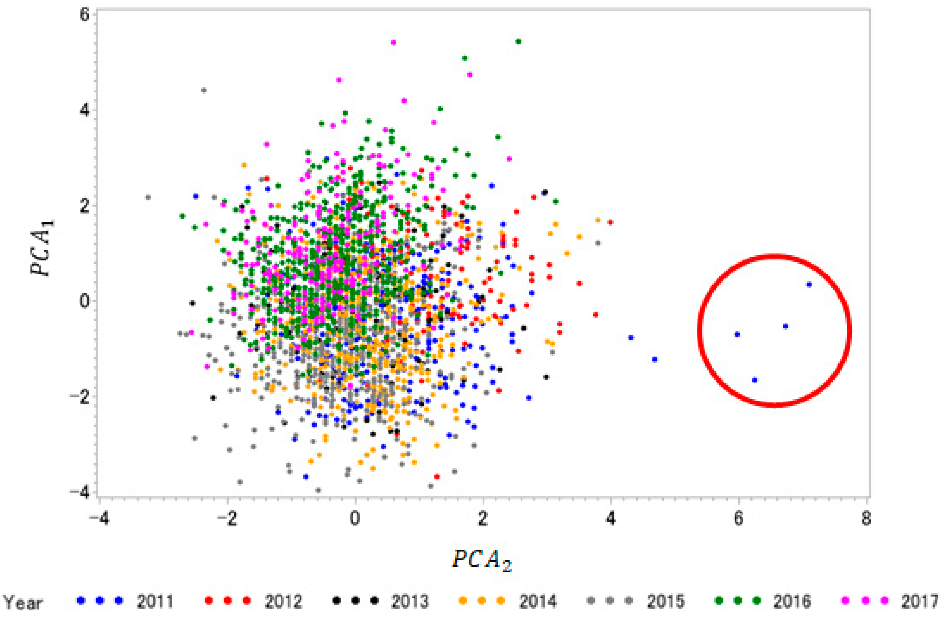
Collectively, these observations suggest that these two PCAs can be used as indices to distinguish apparent improved chemical composition quality as a result of reduced yield and lower starch deposition (unfavorable) from actual improved chemical composition in conjunction with higher yields (favorable). Arithmetic means of the PCAs showed that positive mean values for PCA1 occurred in 2012, 2016, and 2017, whereas positive mean values for PCA2 occurred in 2011–2013 (Table 4; Figure 1). Four outliers from 2011 with extreme PCA2 values were discovered in the scatterplot and were removed prior to stepwise regression analyses (Figure 1).
3.2. Stepwise Regression with Weather and Climatic Variables
Linear regression models were fit for PCA1, PCA2, and yield. A summary of all variables included in each of these three models can be found in Table 1. All three models included the covariate that accounted for the protein-rich germplasm grown in the Dakotas, the AI, the average temperature at flowering, and the average temperature during grain fill. None of the models included GDD or the average temperature during early vegetative growth. It stands to reason that GDD would not likely be included in the regression models due to its collinearity with the average and minimum temperature during grain fill, these latter variables often being included in the regression model. Given that the covariate accounting for the Dakotas is somewhat correlated with the other weather and climatic predictors, it was not interpreted in analyses below [43]. Rather, it is included in the model only to improve the model’s predictive ability.
3.2.1. PCA1—High Grain Protein and Oil
More positive values of PCA1 were the result of higher protein and oil concentrations as opposed to starch concentration, irrespective of whether that increase was due to actual grain quality improvement or a reduced starch concentration and lower yields. More positive values of PCA1 are ideal if attempting to determine which weather conditions lead to more favorable concentrations of protein and oil. The most important predictor in explaining PCA1 was the total precipitation during early vegetative growth, with a partial R2 of 5.1%. The addition of five other predictor variables, namely the average temperature during flowering, the AI, the total precipitation during grain fill, the covariate accounting for the Dakotas, and the average temperature during grain fill (in order of addition to the model using stepwise selection), led to a final model R2 of 12.7%. Given that nothing is known of the specific production management strategies employed or the specific hybrids used, this is a reasonably accurate model. Wet conditions during early growth resulted in reduced PCA1 values, most likely due to nitrogen fertilizer leaching or denitrification and a reduced grain protein concentration [44]. Hot mean temperatures during flowering and grain fill as well as more arid climates resulted in more positive PCA1 values, likely due to drought and heat stress reducing photosynthesis, resulting in reduced starch deposition [45,46,47]. However, PCA1 is a function of both protein and oil, and both of these constituents were found to be at higher concentrations in the grain during favorable-yielding years. More positive values of PCA1 were also observed when sufficient water was available during grain fill. Having an optimal balance of N availability and photoassimilates in a non-water-limiting environment can lead to larger maize kernels with a concurrent higher level of protein [48].
3.2.2. PCA2—High Grain Protein Over Oil
More positive values of PCA2 are the result of higher grain protein as opposed to oil concentration, having already accounted for the chemical composition differences captured by PCA1. Thus, PCA2 is instrumental in describing stressful conditions which influence compositional grain quality. More positive values of PCA2 are indicative of a higher protein concentration as a result of stressful conditions, either drought or heat stress, that decrease starch and oil deposition in the grain. Heat stress during grain fill has been found to decrease kernel oil concentration in semi-dent hybrids [49]. As such, more negative values of PCA2 are ideal for greater yield and oil, but this measure alone will not capture favorable protein concentrations without also examining PCA1. The final regression model for PCA2 had a model R2 of 18.9%, which is moderate (multiple correlation coefficient = 0.453). More negative values of PCA2 were the result of less arid environments where the SWS was also greater. More negative values of PCA2 were also observed in environments with lower temperatures during flowering and grain fill and with greater precipitation during flowering. The average minimum temperature during grain fill was also included in the regression model to improve the predictive ability of the model, but was unnecessary due to the high degree of multicollinearity between the two temperature variables during grain fill.
3.2.3. Yield
Interestingly, even though nothing is known of the specific production management strategies used during the growing season of these samples, the regression of yield against the climatic and weather predictor variables explained 47.7% of the total variability in yield, which is fairly high (multiple correlation coefficient = 0.69). Nine of the eleven possible predictor variables were included in the model, the two that were not included being the average temperature during early vegetative growth and the GDD. In general, yield was higher under growing conditions where ample moisture was available during flowering and grain fill, and where drought was less likely to be a limiting factor due to SWS, AI, or hot temperatures during flowering and grain fill. Too much precipitation early in the growing season was found to decrease yield, likely due to the loss of nitrogen fertilizer from the soil environment. The final model was capable of predicting the average county yields to within 0.89 metric tons/hectare (14 bushels/acre), as a median (Table S3). An alternative measure of model accuracy, the root mean square error (RMSE), was found to be 1.44 metric tons/hectare (23 bushels/acre) in this study. By comparison, the USDA WASDE model, a computationally intensive model that makes use of weather data and satellite imagery to compute multivariate non-linear predictive models for grain yield, was recently shown to have an RMSE of 1.11 metric tons per hectare (18 bushels/acre) early in the growing season [5].
Thus, even though the model we show here is computationally simple, it is similar in accuracy to much more complex models such as the USDA WASDE. Furthermore, it highlights the importance of minimizing drought stress at flowering and grain fill. Otherwise, both yield and grain quality will suffer. Our linear models serve as a foundation for more complex models in the future by indicating (i) maize yield and maize quality are dependent on a shared set of conditions during critical growth periods, and (ii) these critical growth periods should be given greater weight in complex predictive models for the multivariate prediction of yield and compositional quality. As a second consideration, the more complex nonlinear models that are characterized by a higher predictive ability are also characterized by predictor variables that are all highly intercorrelated, meaning that their parameter estimates should not be interpreted [43]. Given that one of our goals was to identify which of the putative critical growth stages are important influencers of grain yield and chemical composition, it was imperative to build models that were characterized by both low multicollinearity and adequate predictive ability. The models presented here, particularly those for PCA2 and yield, accomplish that goal.
3.3. Multivariate Clustering Analysis by ASD
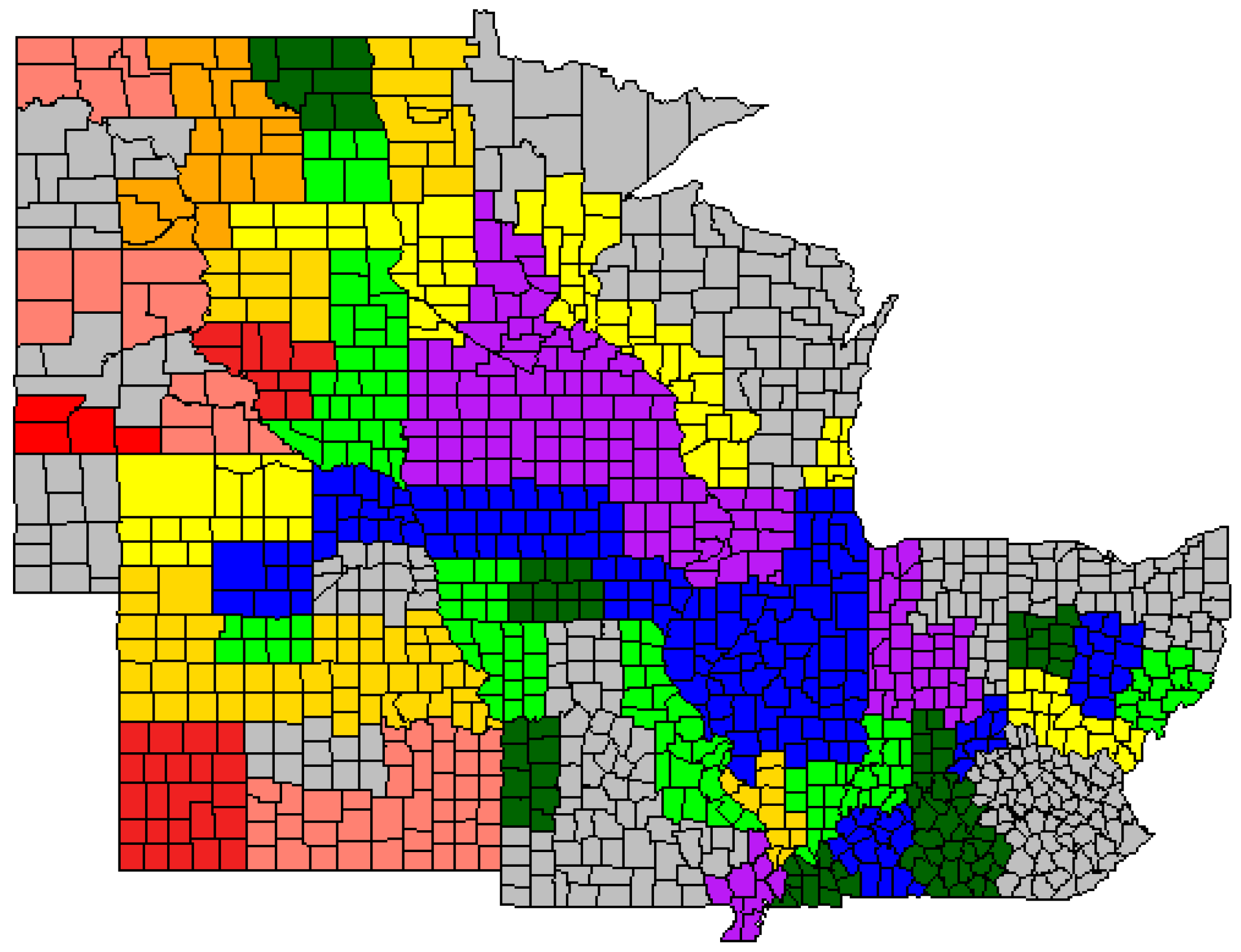
Cluster analysis using Ward’s Minimum Variance Approach indicated that the 76 ASDs used in this study could be subdivided into 10 clusters based on their standardized average PCA1, PCA2, and yield values. These clusters are indicated by different colors in Figure 2.
In Figure 2, a color-spectrum approach was used to visualize the multivariate presentation of yield and the PCAs, as is described in more detail in Table 5. No one cluster of ASDs was ideal; all had their advantages and disadvantages (Table 5). While Cluster 1 (purple) and Cluster 2 (blue) undeniably had the highest yielding averages, the samples from Cluster 2 had somewhat better chemical composition quality overall but slightly less yield.
Overall, ASDs clustered together as one might expect based on similar weather and climatic conditions. The historically high-yielding regions of Iowa, Illinois, and Southern Minnesota fell into Clusters 1 and 2, and ASDs from clusters described by moderate values of all three response variables (green and yellow clusters) falling adjacent to these regions. The ASDs in the Plains States in the west typically fell into more protein rich clusters, but at the expense of reduced yield and oil concentration. Given the aridity of these regions and the frequency of drought conditions, this is to be expected. However, there were three ASDs (NE 30, NE 50, and MO 90) that fell into clusters that were somewhat different than might be expected given their geographical location and the cluster assignments of the neighboring ASDs. Upon further examination, it was noted that these three ASDs all lie in regions where cropland is heavily irrigated (Figure S3). Therefore, it is probable that the improved yields and chemical composition of the grain sampled from these ASDs is due in at least part to the presence of irrigation [50]. Other ASDs of interest are KY 20, IN 90, and OH 50. These ASDs fell into Cluster 2, this cluster typically being reserved for ASDs in the major maize growing regions of Iowa and Illinois. All three of these ASDs are located in areas with a greater presence of rivers than is typical of most of the ASDs included in this study [51]. Thus, these observations lead us to conclude that grain yield and grain chemical composition can be modeled and improved simultaneously, and the key factor involved is non-limited water conditions during flowering and grain fill.
Based on these results, it is apparent that water availability as a function of total rainfall, temperature, AI, and SWS is a major predictor of grain compositional quality and yield. Too much rainfall during early vegetative growth leads to reduced protein concentration and yield, most likely as a result of nitrogen leaching or denitrification. On the other hand, water availability during the two critical growth stages of flowering and grain fill is largely responsible for both grain yield and compositional quality, as indicated by both the multiple regression models and clustering analyses used in this study. Previous studies have also found that irrigation has a greater impact on maize yield than temperature over the season [50]. These findings may be used to predict when weather conditions may hinder yield and/or compositional quality of the grain and could also be used to build more sophisticated models (e.g., nonlinear multivariate models, spatial error models, etc.) that have a stronger weight on the weather conditions at the identified critical growth stages. Ultimately, these findings indicate that both yield and grain compositional quality can be monitored and improved simultaneously, that improved maize grain chemical composition as a result of favorable environmental conditions can be distinguished from superficial, apparent improvement as the result of low-yielding environmental conditions, and that the key limiter to improving grain yield and compositional quality is access to water.
Supplementary Materials
The following are available online at https://www.mdpi.com/2073-4395/9/1/16/s1, Figure S1: Sampling information by ASD, Figure S2: Plot of starch-to-protein ratio by state, Figure S3: Map of irrigation prevalence in the United States, Table S1: Pearson correlation coefficients between test weight and other response variables across seven years of study, Table S2: Vector loadings of PCAs, Table S3: Absolute differences in observed versus predicted, Supplemental Code: R code for latitude and longitude coordinates.
Author Contributions
Conceptualization, J.R.S. and F.E.B.; methodology, L.S.; statistical methodology and formal analysis, C.J.B.-W.; investigation, J.R.S.; resources, F.E.B.; data curation, L.S.; cross-database dataset compilation, C.J.B.-W.; writing—original draft preparation, C.J.B.-W. and J.R.S.; writing—review and editing, J.R.S.; visualization, C.J.B.-W.; supervision, F.E.B.; project administration, J.R.S.; funding acquisition, F.E.B.
Funding
This research was made possible with partial funding from the United States Department of Agriculture National Institute of Food and Agriculture project NC-1200 “Regulation of Photosynthetic Processes” and the Illinois Agriculture Experiment Station project 802-906. This project also would not have been possible without the data collection and analysis support of the U.S. Grains Council (http://grains.org).
Acknowledgments
The authors with to thank Centrec Consulting Group, LLC. for coordinating sample acquisition, analysis, and data compilation.
Conflicts of Interest
The authors declare no conflict of interest.
References
- U.S. Census Bureau. U.S. Exports to World Total by 5-Digit End-Use Code. Available online: https://www.census.gov/foreign-trade/statistics/product/enduse/exports/c0000.html (accessed on 20 August 2018).
- USDA ERS. Corn and Other Feedgrains: Background. Available online: https://www.ers.usda.gov/topics/crops/corn-and-other-feedgrains/background/ (accessed on 20 August 2018).
- U.S. Grains Council. Corn Reports. Available online: https://grains.org/corn_report/ (accessed on 31 July 2018).
- Wilhelm, E.P.; Mullen, R.E.; Keeling, P.L.; Singletary, G.W. Heat stress during grain filling in maize: Effects on kernel growth and metabolism. Crop Sci. 1999, 39, 1733–1741. [Google Scholar] [CrossRef]
- Peng, B.; Guan, K.; Pan, M.; Li, Y. Benefits of seasonal climate prediction and satellite data for forecasting US maize yield. Geophys. Res. Lett. 2018, 45, 9662–9671. [Google Scholar] [CrossRef]
- Lecerf, R.; Ceglar, A.; López-Lozano, R.; Van Der Velde, M.; Bauruth, B. Assessing the information in crop model and meteorological indicators to forecast crop yield over Europe. Agric. Syst. 2019, 168, 191–202. [Google Scholar] [CrossRef]
- Warren, F.B. Forecasting corn ear weights from daily weather data. In Proceedings of the Conference Applied Statistics in Agriculture, Manhattan, KS, USA, 30 April–2 May 1989. [Google Scholar] [CrossRef]
- Alexander, D.E. Breeding special nutritional and industrial types. In Corn and Corn Improvement, 3rd ed.; Sprague, G., Dudley, J., Eds.; ASA-CSSA-SSSA: Madison, WI, USA, 1988. [Google Scholar]
- Thomison, P.R.; Geyer, A.B.; Lotz, L.D.; Siegrist, H.J.; Dobbels, T.L. Topcross high oil corn production: Select grain quality attributes. Agron. J. 2003, 95, 147–154. [Google Scholar] [CrossRef]
- Uribelarrea, M.; Below, F.E.; Moose, S.P. Grain composition and productivity of maize hybrids derived from the Illinois Protein Strains in response to variable nitrogen supply. Crop Sci. 2004, 44, 1593–1600. [Google Scholar] [CrossRef]
- USDA ERS. Corn and Other Feedgrains: Trade. Available online: https://www.ers.usda.gov/topics/crops/corn-and-other-feedgrains/trade/ (accessed on 20 August 2018).
- Butts-Wilmsmeyer, C.J.; Mumm, R.H.; Bohn, M.O. Concentration of beneficial phytochemicals in harvested grain of US yellow dent maize (Zea mays L.) germplasm. J. Agric. Food Chem. 2017, 65, 8311–8318. [Google Scholar] [CrossRef] [PubMed]
- Cook, J.P.; McMullen, M.D.; Holland, J.B.; Tian, F.; Bradbury, P.; Ross-Ibarra, J.; Buckler, E.S.; Flint-Garcia, S.A. Genetic architecture of maize kernel composition in the nested association mapping and inbred association panels. Plant Physiol. 2012, 158, 824–834. [Google Scholar] [CrossRef] [PubMed]
- Lejeune, P.; Bernier, G. Effect of environment on the early steps of ear initiation in maize (Zea mays L.). Plant Cell Environ. 1996, 19, 217–224. [Google Scholar] [CrossRef]
- Cantarero, M.G.; Cirilo, A.G.; Andrade, F.H. Night temperature at silking affects kernel set in maize. Crop Sci. 1999, 39, 703–710. [Google Scholar] [CrossRef]
- Edreira, J.I.R.; Carpici, E.B.; Sammarro, D.; Otegui, M.E. Heat stress effects around flowering on kernel set of temperate and tropical maize hybrids. Field Crops Res. 2011, 123, 62–73. [Google Scholar] [CrossRef]
- Prasad, P.V.V.; Bheemanahalli, R.; Jagadish, S.V.K. Field crops and the fear of heat stress-opportunities, challenges and future directions. Field Crops Res. 2017, 200, 114–121. [Google Scholar] [CrossRef]
- Jones, R.J.; Gengenbach, B.G.; Cardwell, V.B. Temperature effects on in vitro kernel development of maize. Crop Sci. 1981, 21, 761–766. [Google Scholar] [CrossRef]
- Seebauer, J.R.; Singletary, G.W.; Krumpelman, P.M.; Ruffo, M.L.; Below, F.E. Relationship of source and sink in determining kernel composition of maize. J. Exp. Bot. 2010, 61, 511–519. [Google Scholar] [CrossRef] [PubMed]
- Singletary, G.W.; Banisadr, R.; Keeling, P.L. Heat-stress during grain filling in maize—effects on carbohydrate storage and metabolism. Aust. J. Plant Physiol. 1994, 21, 829–841. [Google Scholar] [CrossRef]
- Abe, A.; Menkir, A.; Moose, S.P.; Adetimirin, V.O.; Olaniyan, A.B. Genetic variation for nitrogen-use efficiency among selected tropical maize hybrids differing in grain yield potential. J. Crop Improv. 2013, 27, 31–52. [Google Scholar] [CrossRef]
- Blackmer, A.M.; Pottker, D.; Cerrato, M.E.; Webb, J. Correlations between soil nitrate concentrations in late spring and corn yields in Iowa. J. Prod. Agric. 1989, 2, 103–109. [Google Scholar] [CrossRef]
- Jeong, H.; Bhattarai, R. Exploring the effects of nitrogen fertilization management alternatives on nitrate loss and crop yields in tile-drained fields in Illinois. J. Environ. Manag. 2018, 213, 341–352. [Google Scholar] [CrossRef]
- Mastrodomenico, A.T.; Hendrix, C.C.; Below, F.E. Nitrogen use efficiency and the genetic variation of maize expired plant variety protection germplasm. Agriculture 2018, 8, 3. [Google Scholar] [CrossRef]
- Seebauer, J.R.; Moose, S.P.; Fabbri, B.J.; Crossland, L.D.; Below, F.E. Amino acid metabolism in maize earshoots. Implications for assimilate preconditioning and nitrogen signaling. Plant Physiol. 2004, 136, 4326–4334. [Google Scholar] [CrossRef]
- Archontoulis, S.V.; Miguez, F.E.; Moore, K.J. Evaluating APSIM maize, soil water, soil nitrogen, manure, and soil temperature modules in the midwestern United States. Agron. J. 2014, 106, 1025–1040. [Google Scholar] [CrossRef]
- Yang, X.L.; Lu, Y.L.; Tong, Y.A.; Yin, X.F. A 5-year lysimeter monitoring of nitrate leaching from wheat-maize rotation system: Comparison between optimum N fertilization and conventional farmer N fertilization. Agric. Ecosyst. Environ. 2015, 199, 34–42. [Google Scholar] [CrossRef]
- Troyer, A.F. Adaptedness and heterosis in corn and mule hybrids. Crop Sci. 2006, 46, 528–543. [Google Scholar] [CrossRef]
- Illinois Crop Improvement Association. Grain Laboratory Services. Available online: https://www.ilcrop.com/labservices/grainservices (accessed on 20 January 2018).
- USDA NASS. Quick Stats. Available online: https://quickstats.nass.usda.gov/ (accessed on 1 August 2018).
- Becker, R.A.; Wilks, A.R.; Brownrigg, R.; Minka, T.P.; Deckmyn, A. Maps: Draw Geographical Maps. R Package Version 3.3.0. Available online: https://CRAN.R-project.org/package=maps (accessed on 15 August 2018).
- Chapman, K.; McGuire, J. NutrientStar TED Framework Tool. Available online: http://nutrientstar.org/ted-framework/ (accessed on 31 July 2018).
- USDA NASS. County Data Frequently Asked Questions. Available online: https://www.nass.usda.gov/Data_and_Statistics/County_Data_Files/Frequently_Asked_Questions/index.php# (accessed on 20 July 2018).
- USDA NASS. Charts and Maps. Available online: https://www.nass.usda.gov/Charts_and_Maps/Crops_County/boundary_maps/indexgif.php (accessed on 20 July 2018).
- Midwestern Regional Climate Center. Cli-Mate: Daily County Data between Two Dates. Available online: https://mrcc.illinois.edu/CLIMATE/ (accessed on 20 July 2018).
- Johnson, D.E. Principal component analysis. In Applied Multivariate Methods for Data Analysts; Brooks/Cole Publishing Company: Pacific Grove, CA, USA, 1998; pp. 110–111. [Google Scholar]
- Butts-Wilmsmeyer, C.J.; Mumm, R.H.; Rausch, K.; Kandhola, G.; Yana, N.A.; Happ, M.M.; Ostezan, A.; Wasmund, M.; Bohn, M.O. Changes in phenolic acid content in maize during food product processing. J. Agric. Food Chem. 2018, 66, 3378–3385. [Google Scholar] [CrossRef] [PubMed]
- Labate, J.A.; Lamkey, K.R.; Mitchell, S.E.; Kresovich, S.; Sullivan, H.; Smith, J.S.C. Molecular and historical aspects of corn belt dent diversity. Crop Sci. 2003, 43, 80–91. [Google Scholar] [CrossRef]
- Li, P.X.P.; Hardacre, A.K.; Campanella, O.H.; Kirkpatrick, K.J. Determination of endosperm characteristics of 38 corn hybrids using the Stenvert Hardness test. Cereal Chem. 1996, 73, 466–471. [Google Scholar]
- Brown, W.L.; Zuber, M.S.; Darrah, L.L.; Glover, D.V. Origin, adaptation, and types of corn. In National Corn Handbook; Cooperative Extension Service, Iowa State Univ.: Ames, IA, USA, 1985; pp. 1–6. [Google Scholar]
- Gayral, M.; Gaillard, C.; Bakan, B.; Dalgalarrondo, M.; Elmorjani, K.; Delluc, C.; Brunet, S.; Linossier, L.; Morel, M.H.; Marion, D. Transition from vitreous to floury endosperm in maize (Zea mays L.) kernels is related to protein and starch gradients. J. Cereal Sci. 2016, 68, 148–154. [Google Scholar] [CrossRef]
- Kereliuk, G.R.; Sosulski, F.W. Properties of corn samples varying in percentage of dent and flint kernels. Food Sci. Technol. Leb.-Wiss. Technol. 1995, 28, 589–597. [Google Scholar] [CrossRef]
- Kutner, M.H.; Nachtsheim, C.J.; Neter, J.; Li, W. Applied linear statistical models. In Applied Linear Statistical Models, 5 ed.; Gordon, B., Hercher, R.T., Eds.; McGraw-Hill: New York, NY, USA, 2005. [Google Scholar]
- Dinnes, D.L.; Karlen, D.L.; Jaynes, D.B.; Kaspar, T.C.; Hatfield, J.L.; Colvin, T.S.; Cambardella, C.A. Nitrogen management strategies to reduce nitrate leaching in tile-drained midwestern soils. Agron. J. 2002, 94, 153–171. [Google Scholar] [CrossRef]
- Dwyer, L.M.; Stewart, D.W.; Tollenaar, M. Analysis of maize leaf photosynthesis under drought stress. Can. J. Plant Sci. 1992, 72, 477–481. [Google Scholar] [CrossRef] [Green Version]
- Lobell, D.B.; Field, C.B. Global scale climate—Crop yield relationships and the impacts of recent warming. Environ. Res. Lett. 2007, 2, 014002. [Google Scholar] [CrossRef]
- Nielson, B.L. Warm Nights & High Yields of Corn: Oil & Water? Available online: https://www.agry.purdue.edu/ext/corn/news/timeless/WarmNights.html (accessed on 22 August 2018).
- Below, F.E.; Cazetta, J.O.; Seebauer, J.R. Carbon/nitrogen interactions during ear and kernel development of maize. In Physiology and Modeling Kernel Set in Maize; Westgate, M., Boote, K., Eds.; Crop Science Society of America and American Society of Agronomy: Madison, WI, USA, 2000; pp. 15–24. [Google Scholar] [CrossRef]
- Mayer, L.I.; Edreira, J.I.R.; Maddonni, G.A. Oil yield components of maize crops exposed to heat stress during early and late grain-filling stages. Crop Sci. 2014, 54, 2236–2250. [Google Scholar] [CrossRef]
- Carter, E.K.; Melkonian, J.; Riha, S.J.; Shaw, S.B. Separating heat stress from moisture stress: Analyzing yield response to high temperature in irrigated maize. Environ. Res. Lett. 2016, 11, 094012. [Google Scholar] [CrossRef]
- Glelck, P.; Heberger, M. American Rivers: A Graphic. Available online: http://pacinst.org/american-rivers-a-graphic/ (accessed on 24 October 2018).
Figure 1.
Scatterplot of PCAs by year. Different years are represented by different colors. Four outliers were identified for removal based on the PCA, these being circled in red in the figure above. Years 2016 and 2017, represented by green and magenta points, respectively, were both high yielding years characterized by higher protein and oil concentrations. These two years separate from the other years in the scatterplot, suggesting that these two PCAs could be used to characterize improved compositional grain quality and yield simultaneously.

Figure 2.
Multivariate clustering analysis by ASD. The ASDs with the same color fall in the same cluster and have similar maize yield and compositional quality. A color-spectrum approach was used to represent the clusters, with purple being high yielding ASDs with lower protein content. Blue is high yielding with decent compositional quality. The greens and yellows are used to describe ASDs with moderate yield and compositional quality values. Lastly, the orange and progressively red ASDs represent areas where protein concentration is higher, but at the expense of yield.


Table 1.
Description of weather and climatic predictor variables and their utilization in models.
| Xik | Acronym | General Description | Models Where Included | ||
|---|---|---|---|---|---|
| PCA1 | PCA2 | Yield | |||
| Xi1 | EGP | The total precipitation during the early vegetative growth stage in inches | Y | N | Y |
| Xi2 | EGT | The average daily temperature during the early vegetative growth stage in °F | N | N | N |
| Xi3 | FP | The total precipitation during the flowering growth stage in inches | N | Y | Y |
| Xi4 | FT | The average daily temperature during flowering in °F | Y | Y | Y |
| Xi5 | GFP | The total precipitation during grain fill in inches | Y | N | Y |
| Xi6 | GFT | The average daily temperature during grain fill in °F | Y | Y | Y |
| Xi7 | GFMT | The average minimum daily temperature during grain fill in °F | N | Y | Y |
| Xi8 | SWS | Soil water storage, more positive values indicate a greater soil water storage capacity | N | Y | Y |
| Xi9 | AI | The aridity index, smaller values indicate a more arid environment as a function of average annual precipitation and rate of evapotranspiration | Y | Y | Y |
| Xi10 | GDD | The average growing degree days for an area | N | N | N |
| Xi11 | D | A qualitative covariate accounting for the greater protein content typical of hybrids grown in the Dakotas. This variable was assigned a value of 0 if the sample in question came from either ND or SD and a value of 1 otherwise. | Y | Y | Y |
Table 2.
Pearson correlation coefficients between weather and climate predictor variables. Correlations which surpassed the threshold for multicollinearity concerns (|r| ≥ 0.50) are highlighted in orange. Other correlations of moderate strength are shown in blue.
Table 2.
Pearson correlation coefficients between weather and climate predictor variables. Correlations which surpassed the threshold for multicollinearity concerns (|r| ≥ 0.50) are highlighted in orange. Other correlations of moderate strength are shown in blue.
| EGP † | EGT | FP | FT | GFP | GFT | GFMT | SWS | GDD | AI | |
|---|---|---|---|---|---|---|---|---|---|---|
| 0.132 | −0.175 | −0.110 | −0.019 | −0.243 | −0.193 | 0.006 | −0.025 | −0.004 | EGP | |
| −0.260 | 0.169 | −0.058 | 0.221 | 0.213 | −0.086 | 0.520 | 0.442 | EGT | ||
| 0.019 | 0.153 | 0.150 | 0.237 | −0.060 | −0.003 | 0.099 | FP | |||
| −0.175 | 0.496 | 0.420 | 0.098 | 0.373 | 0.004 | FT | ||||
| 0.084 | 0.203 | 0.024 | 0.049 | 0.207 | GFP | |||||
| 0.953 | 0.029 | 0.701 | 0.261 | GFT | ||||||
| 0.001 | 0.693 | 0.346 | GFMT | |||||||
| 0.011 | −0.178 | SWS | ||||||||
| 0.479 | GDD |
† EGP, early growth precipitation; EGT, early growth temperature; FP, flowering period precipitation; FT, flowering period daily average temperature; GFP, precipitation during grain fill; GFT, average temperature during grain fill; GFMT, Average minimum temperature during grain fill; SWS, soil water storage capacity; GDD, average growing degree days for an area; AI, aridity index.
Table 3.
Pearson correlation coefficients between response variables. Correlations that surpassed the threshold for inclusion in PCA (|r| ≥ 0.50) are highlighted in orange. Other correlations of moderate strength are shown in blue.
Table 3.
Pearson correlation coefficients between response variables. Correlations that surpassed the threshold for inclusion in PCA (|r| ≥ 0.50) are highlighted in orange. Other correlations of moderate strength are shown in blue.
| Grain Concentration | Test | |||||
|---|---|---|---|---|---|---|
| Protein | Starch | Oil | Weight | PCA1 | PCA2 | |
| Yield | −0.431 | 0.063 | 0.248 | 0.176 | −0.087 | −0.488 |
| Protein | −0.544 | −0.001 | −0.018 | NA† | NA | |
| Starch | −0.599 | 0.176 | NA | NA | ||
| Oil | −0.070 | NA | NA | |||
| Test Weight | −0.126 | 0.034 | ||||
| PCA1 | 0.000 | |||||
† NA, Not applicable.
Table 4.
Average maize grain chemical composition, PCA, and yield values between 2011 to 2017 for U.S. Corn Belt samples with and without the Dakota states.
Table 4.
Average maize grain chemical composition, PCA, and yield values between 2011 to 2017 for U.S. Corn Belt samples with and without the Dakota states.
| Grain Concentration | ||||||
|---|---|---|---|---|---|---|
| Year | Protein | Starch | Oil | PCA1 | PCA2 | Yield |
| ————g/kg———— | T/ha | |||||
| All States Included | ||||||
| 2011 | 87.2 | 734.7 | 36.7 | −0.40 | 0.49 | 8.93 |
| 2012 | 94.4 | 731.6 | 37.5 | 0.42 | 1.03 | 7.19 |
| 2013 | 85.8 | 734.1 | 38.5 | −0.17 | 0.03 | 10.00 |
| 2014 | 84.6 | 735.0 | 37.6 | −0.43 | 0.07 | 10.86 |
| 2015 | 81.9 | 736.9 | 37.7 | −0.75 | −0.19 | 10.86 |
| 2016 | 85.7 | 724.7 | 40.4 | 0.84 | −0.32 | 10.97 |
| 2017 | 86.2 | 723.2 | 41.2 | 1.09 | −0.42 | 10.75 |
| Excluding Dakotas | ||||||
| 2011 | 86.8 | 734.8 | 36.8 | −0.41 | 0.43 | 9.41 |
| 2012 | 94.3 | 731.6 | 37.5 | 0.41 | 1.01 | 7.46 |
| 2013 | 85.8 | 734.1 | 38.5 | −0.17 | 0.03 | 10.00 |
| 2014 | 83.8 | 735.6 | 37.9 | −0.50 | −0.05 | 11.51 |
| 2015 | 81.0 | 737.4 | 37.8 | −0.82 | −0.29 | 11.00 |
| 2016 | 84.9 | 725.6 | 40.2 | 0.70 | −0.36 | 11.22 |
| 2017 | 85.9 | 723.6 | 41.1 | 1.04 | −0.43 | 11.45 |
Table 5.
Means of response variables and number of ASDs included for each cluster of maize grain quality and quantity relationship to weather from 2011–2017. Blue cells represent more desirable means and orange cells represent less desirable means for PCA1 (relatively high protein and oil concentrations), PCA2 (more protein than oil), and yield. Yield is presented in metric tons per hectare with bushels per acre in parentheses.
| Cluster | Color | ASD † Count | PCA1 | PCA2 | Yield |
|---|---|---|---|---|---|
| 1 | Purple | 13 | −0.44397 | 0.09525 | 11.214 (178.644) |
| 2 | Blue | 14 | 0.1441 | −0.17026 | 10.840 (172.674) |
| 3 | Green | 12 | 0.19138 | 0.33464 | 9.186 (146.339) |
| 4 | Dark Green | 7 | −0.07588 | −0.10005 | 9.063 (144.381) |
| 5 | Yellow | 9 | −0.73882 | 0.43401 | 10.184 (162.237) |
| 6 | Orange | 8 | 0.72065 | 0.59974 | 8.638 (137.604) |
| 7 | Gold | 3 | 1.52549 | 0.54987 | 6.980 (111.195) |
| 8 | Salmon | 6 | 0.4815 | 0.82565 | 6.564 (104.568) |
| 9 | Brick Red | 3 | 1.30486 | 1.15527 | 9.190 (146.394) |
| 10 | Red | 1 | −1.78707 | 0.90478 | 6.362 (101.340) |
† ASD—Agricultural Statistics District.
© 2019 by the authors. Licensee MDPI, Basel, Switzerland. This article is an open access article distributed under the terms and conditions of the Creative Commons Attribution (CC BY) license (http://creativecommons.org/licenses/by/4.0/).
Share and Cite
MDPI and ACS Style
Butts-Wilmsmeyer, C.J.; Seebauer, J.R.; Singleton, L.; Below, F.E. Weather During Key Growth Stages Explains Grain Quality and Yield of Maize. Agronomy 2019, 9, 16. https://doi.org/10.3390/agronomy9010016
AMA Style
Butts-Wilmsmeyer CJ, Seebauer JR, Singleton L, Below FE. Weather During Key Growth Stages Explains Grain Quality and Yield of Maize. Agronomy. 2019; 9(1):16. https://doi.org/10.3390/agronomy9010016
Chicago/Turabian StyleButts-Wilmsmeyer, Carrie J., Juliann R. Seebauer, Lee Singleton, and Frederick E. Below. 2019. "Weather During Key Growth Stages Explains Grain Quality and Yield of Maize" Agronomy 9, no. 1: 16. https://doi.org/10.3390/agronomy9010016
Note that from the first issue of 2016, this journal uses article numbers instead of page numbers. See further details here.