Implementation of Aerosol-Cloud Interaction within WRF-CHIMERE Online Coupled Model: Evaluation and Investigation of the Indirect Radiative Effect from Anthropogenic Emission Reduction on the Benelux Union

Abstract

The indirect effects of aerosol are particularly important over regions where meteorological conditions and aerosol content are favourable to cloud formation. This was observed during the Intensive Cloud Aerosol Measurement Campaign (IMPACT) (European Integrated project on Aerosol Cloud Climate and Air quality Interaction (EUCAARI) project) in the Benelux Union during May 2008. To better understand this cloud formation variability, the indirect effects of aerosol have been included within the WRF-CHIMERE online model. By comparing model results to the aircraft measurements of IMPACT, to surface measurements from EMEP and AIRBASE and to MODIS satellite measurements, we showed that the model is able to simulate the variability and order of magnitude of the observed number of condensation nuclei (CN), even if some differences are identified for specific aerosol size and location. To quantify the impact of the local anthropogenic emissions on cloud formation, a sensitivity study is performed by halving the surface emissions fluxes. It is shown that the indirect radiative effect (IRE) at the surface is positive for both shortwave and longwave with a net warming of +0.99 W/m². In addition, important instantaneous changes are modelled at local scale with up to ±6 °C for temperatures and ±50 mm/day for precipitation.

1. Introduction

Meteorological and chemical processes influence each other and aerosols affect directly and indirectly both the weather and climate [1]. The direct effect arises from aerosol properties of scattering and absorbing both sunlight and thermal infrared radiation [2,3]. Aerosol also affects the properties of clouds and precipitation rate [4]. The last one is usually referred as “indirect effect” and arises from the fact that aerosols act as cloud condensation nuclei (CCN). An increase of CCN, for clouds of equal liquid water content (LWC), enhances the concentration of cloud droplets and reduces their size. This results in a cloud albedo increase and is called “first indirect effect”, “albedo effect” or “Twomey’s effect” [5,6]. Aerosols affect cloud thickness and lifetime, hence precipitations, through the “second indirect effect” or “Albrecht effect” [7,8,9].

In addition, aerosols may act as ice nuclei (IN) contributing to the “glaciation indirect effect”. An increase of IN leads to the enhancement of ice crystal concentration in the midlevel clouds due to heterogeneous freezing (−5 > T > −30 °C), resulting in more precipitation and shorter cloud lifetime [10,11]. It also lowers the number of ice crystals in cirrus clouds, because the earlier onset of ice formation competes with the homogeneous freezing that occurs at high relative humidity on deliquesced aerosol particles at temperatures lower than −36 °C [11]. Therefore, under relatively high values of IN, cirrus form readily, but the lower ice content leads to sedimentation and shorter lifetime. Although many studies have been conducted to assess the impact of the indirect effects, the estimation of the net radiative forcing attributable to aerosol-cloud interactions (ACI) is still highly uncertain with a global estimate of −0.45 (−1.2 to 0.0) W/m² [1].

In the last decade, many meteorology-chemistry online coupled models have been developed in order to represent the complex aerosol-cloud-radiation feedbacks. Several studies have shown that the introduction of ACI in atmospheric models leads to a series of non-linear effects [12] and improves meteorological processes and chemical composition of short-range regional simulations [13,14,15,16,17,18,19,20]. Baklanov et al. [12] distinguish two kinds of coupled models. In the first group, the “online integrated” models, the chemical and meteorological processes are solved on the same grid and same time step. WRF-Chem [21], COSMO-ART [14], Enviro-HIRLAM [22], and RAMS/ICLAMS [23] are “online integrated”. In the second group, “online access” models, meteorological and chemical modules conserve their independence and may run on two different grids, but information is exchanged between models on a regular and frequent basis. WRF-CHIMERE [24], LOTO-EUROS [25], WRF-CMAQ [26], and MEMO-MATS [27] are “online access”.

A significant contribution to climate change is attributed to short-lived pollutants (SLCP) especially at regional scale [1]. Target emission reduction of certain SLCPs could reduce the global warming rate, on a short time scale (e.g., Stohl et al. [28]). Many studies of global warming mitigation strategies were conducted taking into account only the reduction of emissions of some selected aerosol species. These species are usually the aerosols that cause the warming of the atmosphere such as BC [28]. The basic idea is that, given the short lifetime of aerosol particles, a reduction of BC emissions from selected sources may have an immediate benefit on climate (e.g., Bond et al. [29]). On a practical level, it is not easy to reduce the warming aerosol emissions alone because they are co-emitted together to other SLCPs and precursor gases that lead to secondary aerosol formation. The effects of SLCP reduction on the radiative budget were investigated in many studies [28,30,31,32,33] and the quantification of SLCP abatement strategies is affected by many issues that are also related to ACI. As highlighted by Baklanov et al. [34], the indirect effect seems to be very sensitive to the degree of sophistication of the chosen parameterizations and to the detail of the implementation. Model intercomparisons showed that although the models use the same theoretical approach to simulate the ACI, the results obtained may be different [34].

In this work, the implementation of ACI within the WRF-CHIMERE modeling system [24] is described (Section 2) and evaluated (Section 3 and Section 4) over the Benelux Union during the European Integrated project on Aerosol Cloud Climate and Air quality Interaction (EUCAARI) campaign [35]. The simulation of cloud properties is evaluated against MODIS satellite observations (Section 4.5.3). As example of a first application, the regional indirect radiative effect (IRE) exerted by a reduction of anthropogenic emissions on a short period over the Benelux Union has been analyzed at high resolution (4 km) (Section 5).

2. Implementation of the Aerosol-Cloud Interaction within WRF-CHIMERE Online Model

WRF-CHIMERE is an online access model [24]. The Weather Research and Forecasting (WRF) model is a mesoscale non-hydrostatic meteorological model that includes several options for physical parameterizations of the different atmospheric processes (www.wrf-model.org). CHIMERE is a chemistry-transport model suitable for a wide range of atmospheric composition studies extending from urban to hemispheric scale [36].

The online coupling of the two models is described in Briant et al. [25] and is performed by using the version 3.7.1 of WRF and CHIMERE 2017. The models are coupled through an external coupler called OASIS3-MCT [37,38]. The models run on the same horizontal grid but vertical grids are different. The current version of WRF-CHIMERE allows both one and two way coupling. In the one-way coupling, WRF feeds CHIMERE with sub hourly frequency exchanging 28 meteorological variables through the OASIS interface implemented in the models. The two-way interaction includes the aerosol direct effect with CHIMERE sending with sub hourly frequency 23 aerosol optical properties including aerosol optical depth, aerosol single scattering albedo and asymmetry parameter. Aerosol optical properties are diagnosed with Mie theory at different wavelengths starting from the aerosol size distribution predicted by CHIMERE and are used in WRF to force the radiative transfer calculation of both short and longwave radiation through the Rapid Radiative Transfer Model for GCMs (RRTMG) [39]. A detailed description of WRF-CHIMERE for the direct effect is provided by Briant et al. [24].

The two-way coupling was extended to include the indirect aerosol feedback. The Thompson and Eidhammer cloud microphysics scheme [40] (hereinafter referred to as TE14) was used to calculate the cloud droplet nucleation rate. This scheme uses the aerosol particle number concentration field from a multi-year global model simulation. Aerosols are then activated based on a lookup table created using an explicit treatment of the Kohler theory with a lognormal distribution of aerosols. Here the TE14 scheme was adapted to use the CHIMERE aerosol simulations. Since CHIMERE uses a sectional treatment for aerosols, the activation scheme of TE14 has been replaced with the Abdul-Razzak and Ghan [41] parameterization. Given the updraft velocity, size, number concentration and composition of each section, it predicts the fraction of activated aerosol within each section as a function of maximum supersaturation of an adiabatic rising parcel. According to TE14, the aerosol activation as droplet occurs at cloud base as well as anywhere within a cloud if the number of activated aerosols is larger than the existing droplet concentration. Following Ghan et al. [42], the number of aerosols activated as cloud droplet in each section of CHIMERE size distribution is calculated on a maximum supersaturation determined from a Gaussian spectrum of updraft velocity and internally mixed aerosol properties with a similar method adopted in WRF/Chem [43]. In addition to the aerosol activation as cloud droplet at environmental supersaturation, a diagnostic of the supersaturation spectrum of CCN has been implemented in the model. The number of aerosols acting as CCN in each section of CHIMERE size distribution is determined at six levels of supersaturation (0.02, 0.05, 0.1, 0.2, 0.5, and 1%).

Cloud ice formation from heterogeneous and homogeneous nucleation follows the method already implemented in TE14, but the climatology of IN and deliquesced aerosol is replaced with the aerosol particle predicted by CHIMERE. Several aerosol species may act as IN. Observation campaigns have shown the predominant role of dust particles as IN [44,45]. The worldwide sets of observations reported by Hoose et al. [46] show that the contribution of carbonaceous aerosol to IN is variable, it ranges from 0 up to 47%. On the other hand Bond et al. [29], on the basis of the field and laboratory measurements, have highlighted conflicting results on the effective contribution of black carbon (BC) to IN for mixed-phase clouds, while it has a role at best moderate in contributing to IN of ice-phase clouds. Therefore, since the ability of BC to act as IN is not clear, we consider as IN only the accumulated dust particles predicted by CHIMERE with diameter larger than 0.5 µm. The number of INs that nucleate as ice particles through the immersion freezing and deposition is determined by using the parameterization of DeMott et al. [47] that is a modified version of the scheme of De Mott et al. [11]. The freezing of supercooled water by contact nucleation follows Bigg [48] as done by Thompson et al. [49] with the IN concentration that alter the “effective temperature” to freeze the water drops. Homogeneous freezing of deliquesced aerosols is parameterized following Koop et al. [50]. Deliquesced aerosol number concentration is based on the CHIMERE prediction of a mixture of hygroscopic particles (sulphate, nitrate, ammonium, sea salt and secondary organic aerosols) with the diameter larger than 0.1 µm.

In summary, size number distribution, aerosol bulk hygroscopitcity, IN and deliquesced aerosol predicted by CHIMERE are sent to WRF through the coupler OASIS. These fields are used within WRF to calculate the droplet and ice nucleation rates. Cloud droplet and ice number concentration affect both radiative and microphysical processes. Radiative transfer is forced by cloud optical depth calculated starting from predicted cloud droplet and ice effective radius. Moreover, cloud microphysical processes rates are affected by cloud droplet and ice number concentration. Finally, the resulting cloud water content, precipitation rate and cloud optical properties affect the gas and aerosol concentration predicted by CHIMERE through aqueous chemistry, wet scavenging and photolysis.

3. Model Configuration and Setup

3.1. Model Geometry

As shown in Figure 1, the model was configured with three one-way nested domains. The outer domain (D1) has 36 km resolution, domain 2 (D2) 12 km, and inner domain (D3) is cloud resolving at 4 km resolution. D1 extends approximately from latitudes 15° N to 55° N and from longitudes 15° W to 32° E with 150 × 150 grid points. D2 and D3 are centered on the Benelux Union and include 121 × 121 and 166 × 166 nodes, respectively. The reason to have a very wide-ranging domain as D1 is motivated by the need to have an accurate transport of mineral dust because, as will see in Section 4.1, our simulations on D3 are affected by long-range transport of Saharan aerosol dust for a relatively long period. In this study, we used 33 vertical levels extending from surface up to 50 hPa for WRF, and 20 levels up to 200 hPa for CHIMERE. Above CHIMERE top, aerosol concentration exchange between the models are assumed to decrease with an exponential profile. The coupling time (exchange frequency) between models is resolution dependent, it is fixed at 10 min for D1, 6 min for D2, and 5 min for the high resolution domain D3. The coupling frequency increases with the horizontal resolution in order to capture most of the meteorological variability [51].

3.2. Simulation Period

The period simulated in this study extends from 1 to 30 May 2008. This period is splitted into two different periods:

• From 1 to 13 May 2008: this is the spin-up period and the simulation results will not be analyzed.
• From 14 to 30 May 2008: this is the period where the simulation results will be compared to the available measurement. During this analyzed period, different meteorological periods were observed. This leads to different behaviour of the transport, chemistry and, thus, the potential indirect effects of aerosol on clouds. To better understand the following results, this period is divided in four sub-periods as:
  • P1: the day of 15 May 2008
  • P2a: the day of 18 May 2008
  • P2b: the days from 19 to 21 May 2008
  • P3: the days from 26 to 30 May 2008

For these two weeks, a series of 24 h simulations was performed each day starting at 00 UTC. Each simulation is restarted from a 12 h of meteorological pre-forecast starting at 12 UTC the previous day in order to spin-up the meteorology. The choice to re-initialize the WRF model every 24 h instead of performing a continuous run is motivated by the results obtained from preliminary sensitivity tests conducted with WRF offline (no feedback with CHIMERE). These tests have shown that the re-initialization improves the simulation of cloud fields in the cloud resolving domain with respect to a continuous run.

3.3. Parametrizations Used

Parameterizations for meteorological and chemical processes used in this work are listed in

Table 1. Physical and chemical parameterizations used for WRF and CHIMERE.

Processes	WRF-CHIMERE Parameterizations
Cloud Microphysics	Thompson and Eidhammer [40]
Cumulus Cloud	Grell-Freitas [54] (D1 and D2 only)
Longwave radiation	RRTMG
Shortwave radiation	RRTMG
PBL	YSU
Surface Layer	Monin-Obukov
Surface	Noah LSM
Gas-phase Chemistry	MELCHIOR2
Photolysis	Fast-JX
Aerosol Model	Bessagnet et al. [60]
Secondary Organic Aerosol	Bessagnet et al. [61]
Anthropogenic Emissions	HTAP
Biogenic Emissions	MEGAN
Dust Emissions	Menut et al. [65]
Sea Salt Emissions	Monahan [66]

. Main parameterizations used in WRF include the Thompson and Eidhammer [40] aerosol aware cloud microphysics scheme modified as described in Section 2, RRTMG for visible and planetary radiation [39], YSU for planetary boundary layer [52], Noah land surface model [53], and Grell-Freitas [54] for cumulus convection. No cumulus parameterization is used in the cloud resolving domain.

Gas-phase chemical evolution in CHIMERE is simulated using the MELCHIOR2 mechanism [55], a reduced version of MELCHIOR1 [56], including 40 gaseous species and 120 photochemical reactions. Photolytic rates are calculated with the Fast-JX scheme [57,58] as described by Mailler et al. [59]. Aerosol particles in CHIMERE are parameterized with the sectional aerosol model described by Bessagnet et al. [60]. In this study, 10 dimensional bins are used. The aerosol species treated by CHIMERE are sulfate (SO₄), nitrate (NO₃), ammonium (NH₄), black carbon (BC), primary unspeciated aerosol, organic matter (OM) constituted by primary and secondary organic aerosols (POA and SOA), aerosol water, mineral dust and sea salt. SOAs are formed by anthropogenic and biogenic sources as described in Bessagnet et al. [61]. Aerosols are assumed to be in thermodynamic equilibrium calculated with a lookup table as in Menut et al. [62]. Dry deposition velocities of trace gases and aerosols are determined according to Wesely [63] and Zhang et al. [64], respectively. The treatment of in and below clouds wet deposition of gases and aerosols follows Menut et al. [62].

Anthropogenic emissions are from the Hemispheric Transport of Air Pollution (HTAPv2) [65] global inventory as described in Mailler et al. [36]. Biogenic, dust and sea salt emissions are calculated online within CHIMERE. Biogenic emissions are estimated with the model of Emissions of Gases and Aerosols from Nature (MEGAN) [66]. Mineral dust and sea salt emissions are parameterized following Menut et al. [67] and Monahan [68], respectively.

Initial conditions for WRF were provided by 6-hourly operational NCEP analyses at a resolution of 1° × 1°. Meteorological boundary conditions for Domain 1 were taken from NCEP data. On the boundaries of D1, CHIMERE is forced with the climatology of gases and aerosols taken from output of global model LMDZ-INCA [69], while the GOCART model [70] is used for dust boundary conditions. For the inner domains D2 and D3, meteorological and chemical boundary conditions were taken from D1 and D2 simulations, respectively. For all three domains, the chemical initial conditions are restarted from previous run. To improve the meteorological prediction, the spectral nudging toward NCEP analysis of wind, temperature and geopotential has been applied in D1 above 850 hPa with a relaxation time of about 1 h.

4. Model Evaluation

WRF-CHIMERE model including the aerosol indirect feedback is evaluated in cloud resolving domain by using aerosol measurements issued in May 2008 during the Intensive Cloud Aerosol Measurement Campaign (IMPACT) campaign in the frame of European Integrated project on Aerosol Cloud Climate and Air quality interaction (EUCAARI) project [35]. Model results are also evaluated through cloud products of MODIS satellite.

EUCAARI dataset is a state-of-the-art collection of aerosol measurements available in Europe, it is a unique and complete dataset available for model evaluation of ACI and in the past was already used in many modelling studies (e.g., [71,72,73,74,75,76]).

4.1. Meterological Conditions

From a meteorological point of view, May 2008 is divided in two periods. These two periods led to different conditions of aerosol load and composition. During the first two weeks, Europe was dominated by an anticyclonic blocking, whereas the second part of the month was characterized by the passage of frontal systems over Central Europe. An overview of the synoptic situation is provided by Hamburger et al. [77].

As shown in Figure S1, on 14 May a high pressure system was centered over Iceland, maintaining stable weather over Benelux where the 850 hPa wind circulation was from South-East because of a cyclone located over the Atlantic. Later the same day, the anticyclone started to decay and the day after the Atlantic cyclone reached continental Europe through the Bay of Biscay (Figure S2).

On 16 May a depression moved from Scandinavia toward Central Europe and it merged with the Atlantic depression in the first hours of 17 May (Figure S3). Several frontal systems crossed the Benelux Union, resulting in an advection of cold and clean Arctic air through the North Sea towards Central Europe. Starting from 18 May the onset of a North-Esterly anticyclonic field and the entry of Atlantic unstable air on the Mediterranean basin favoured the formation of large depressions over north Italy (Figure S4). The cyclone located over north Italy advected warm and moist air towards Central Europe. At the same time, the Scandinavian depression advected cold air over Central Europe through the North Sea. The convergence line of these different air masses caused unstable weather on the Central Europe until 22 May. The days between 16 and 22 May are referred to as a “scavenging background period” [78].

On 21 May, a cut-off broked-off from Iceland cyclone and reached the Biscay Bay on 24 May forming a deep depression until 30 May (Figure S5). During this period, the resulting mean circulation on the Benelux Union was characterized by a warm and moist Southerly flow that allowed a long-range transport of dust from the Sahara desert [74].

4.2. Ground Based and Aircraft Observations

Aerosol mass measurements were performed at Cabauw Experimental Site for Atmospheric Research (CESAR) observatory. It is a tower located 50 km south of Amsterdam (Figure 2). Aerosol mass concentration of SO₄, NO₃, NH₄, and OM is measured with an aerosol mass spectrometry (AMS) located at 60 m on CESAR tower [78]. In addition, surface measurements of daily inorganic mass concentration, PM_2.5, and PM₁₀ are also available with the EMEP and AIRBASE European networks.

Vertical profiles of aerosol mass concentration, aerosol size distribution, and CCN were collected aboard the French ATR-42 aircraft. In this study, we used the flights performed from 15 to 30 May 2008 within D3. Figure 2 shows the flight tracks; date, number, takeoff and landing time are reported in

Table 2. ATR-42 flights during the IMPACT-EUCAARI campaign from 15 to 31 May 2008. In the Table are reported the date of the research flight (RF), flight number, takeoff and landing time, and period attributed to the flight. Refer to the main text (Section 4.4) for a detailed description of the periods.

Date	RF Number	Take-Off and Landing Time (UTC)	Period
15 May 2008	51	06:19–09:50	P1
15 May 2008	52	11:49–15:06	P1
18 May 2008	53	08:50–11.10	P2a
18 May 2008	54	12:01–14:45	P2a
19 May 2008	55	11:06–14:24	P2b
20 May 2008	56	09:02–11:06	P2b
21 May 2008	57	10:07–12:06	P2b
21 May 2008	58	13:45–15:14	P2b
26 May 2008	59	11:59–15:20	P3
28 May 2008	60	07:54–09:55	P3
28 May 2008	61	13:24–15:40	P3
29 May 2008	62	13:15–14:36	P3
30 May 2008	63	11:26–14:42	P3

. A detailed description of the aircraft campaign and the ATR-42 instrumentation is provided by Crumeyrolle et al. [79]. Aerosol mass concentration of several aerosol species was measured with an AMS, a cloud condensation nuclei counter (CCNC) was used to measure the CCN concentration. Aerosol size distribution of particle in the range of 0.02–0.5 µm was measured with a scanning mobility particle sizer (SMPS), while number size distribution of aerosol larger than 0.1 µm was measured with a passive cavity aerosol spectrometer probe (PCASP).

4.3. Cloud Optical Properties

Model skill in reproducing cloud optical properties was assessed by comparing WRF-CHIMERE output with MODIS L2 cloud products. Model output was sampled at the time of MODIS overpass on the high resolution domain, D3. MODIS and modelled data were regridded and averaged on a same regular grid with horizontal resolution of 5 km. The “Cloud_Phase_Optical_Properties” MODIS product has been used to distinguish liquid and ice cloud [80].

4.4. Metric for Model Evaluation

All ground-based and aircraft measurements described in the previous section have been used to evaluate WRF-CHIMERE performances within the high resolution domain D3. The model skill in reproducing the observations was quantified through the use of some statistical indices as the trimean (TM), the interquantile range (IQR), correlation coefficient (r), mean absolute bias (MB), normalized mean bias (NMB), and normalized mean gross error (NMGE). The indices are defined in Appendix A. The use of TM and IQR instead of the classic mean and standard deviation prevents the model evaluation from being affected by outliers [81]. IQR quantifies the spread of the data around the central tendency given by TM.

Three different periods (P1, P2, and P3) may be identified as a function of the synoptic meteorological situation. P1 is relative to 15 May when an Atlantic cyclone approached the continental Europe. RF51 and RF52 have been attributed to P1 and are representative of clean marine air. P2 is referred to “scavenging background period” (16–22 May). In turn, P2 is divided in two sub periods. P2a (16–18 May) is characterized by advection of cold and clean air, P2b (19–22) by convergence of Northerly cold and Southerly warm air. RF53 and RF54 have been attributed to P2a, RF55, RF56, RF57 and RF58 to P2b. P3 days are relative to long-range transport of dust from Sahara desert (23–30 May). RF59, RF60, RF61, RF62 and RF63 have been assigned to P3.

4.5. Evaluation

4.5.1. Aerosol Mass Concentration

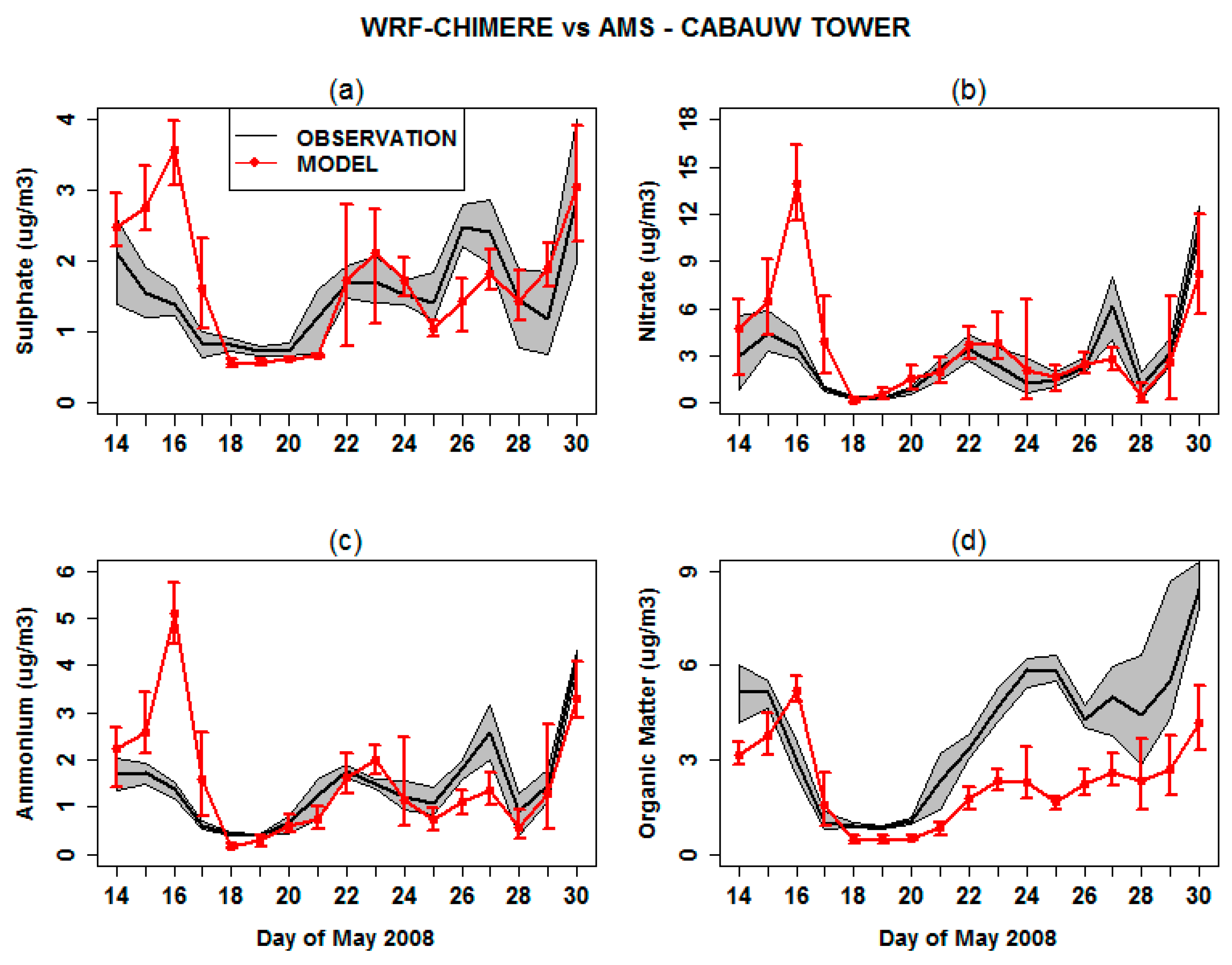
In this subsection we assess the WRF-CHIMERE skill in reproducing the aerosol mass concentration observed at surface and aboard the ATR42. Figure 3 shows the comparison between the observed and predicted time series of daily TM of SO₄, NO₃, NH₄ and OM at Cabauw Tower, with shaded area and red bar denoting the 25th and 75th percentiles. Daily TMs and interquartile ranges are calculated starting from hourly modelled and observed and modelled values. Statistical indices obtained from the comparison are listed in

Table 3. Trimean values (TM), interquantile range (IQR), correlation coefficient (r), mean bias (MB), normalized mean bias (NMB), and normalized mean gross error (NMGE) from the comparison between observed and modelled aerosol sulfate (SO₄), aerosol nitrate (NO₃), aerosol ammonium (NH₄), and organic matter (OM).

Species	TM (IQR) (µg/m3)		r 1	MB 1 (µg/m3)	NMB 1 (%)	NMGE 1 (%)
	OBS	MOD
SO4	1.4 (1.19)	1.6 (0.55)	0.55	0.2	14	38
NO3	2.1 (2.7)	2.9 (0.54)	0.54	0.8	48	77
NH4	1.3 (1.1)	1.3 (0.52)	0.52	0.1	11	52
OM	3.8 (3.8)	2.1 (2.2)	0.64	−1.7	−37	52

¹ Correlation coefficient, MB, NMB and NMGE are calculated between predicated and observed values of daily TM.

.

In general, the model reproduces the day-to-day variations of observations, especially for inorganic aerosols. WRF-CHIMERE captures the marked decrease of the concentrations during the scavenging period, the following recovery starting from 20 May, and the sharp increase of aerosol pollution at the end of month. Model performance is poor on 15–16 May, all three modelled aerosol inorganic species exhibit a peaks 4–5 times larger than observations. This unrealistic modelled peak is not representative of the chemistry and transport ability of the model. For all other days, the model is able to reproduce the observations. For this peak in particular, the fact to have an over-estimation for the three modelled inorganic species and only for one day, shows that the problem is not coming from emissions or chemistry, but more probably to a badly reproduced local wind speed or direction, advecting a polluted air mass just over the tower.

However, correlation between modelled and measured TM is larger than 0.5 for all aerosol species analyzed, it is 0.55, 0.54, 0.52 and 0.64 for SO₄, NO₃, NH₄ and OM, respectively. Despite the overestimation of 15–16 May, NMB of WRF-CHIMERE TM is relatively small for aerosol sulfate (+14%) and ammonium (+11%). Instead, particulate nitrate is overestimated by 48%. TM of OM is underestimated over all simulated periods, MB is −1.7 µg/m³ (or −37%). The analysis of IQR reveals that model spread around central tendency of the distribution is about 1.6 times larger than observed for inorganic aerosols. By contrast, it is 1.7 times lower for OM.

The model tendency to overestimate surface aerosol nitrate is also confirmed by comparison of WRF-CHIMERE simulations with observations of daily inorganic aerosol mass concentration observed at EMEP sites. As shown in

Table 4. As in Table 3, but for mean statistical indices applied to observed and modelled daily mean values at EMEP stations for SO₄, NO₃, NH₄, and AIRBASE sites for PM_2.5 and PM₁₀. N is the number of stations.

Species	N	r	MB (µg/m3)	NMB (%)	MNGE (%)
SO4	5	0.48	−0.2	−14	55
NO3	2	0.70	0.6	247	260
NH4	5	0.56	0.2	44	70
PM2.5	11	0.54	2.4	100	129
PM10	98	0.51	5.6	28	55

, daily NO₃ is highly biased by 0.6 µg/m³ (+247%). As at Cesar tower, modelled SO₄ shows a relative small bias of +14%. Daily aerosol ammonium is overpredicted by 0.2 µg/m³ (+44%). SO₄, NO₃ and NH₄ are reproduced with a correlation of 0.48, 0.70, and 0.56, respectively. These results are statistically comparable with those obtained by large-scale simulation in other modelling studies over Europe. For example, in multi-year simulations of Lecoeur and Seigneur [82] correlation coefficient is 0.57, 0.42, and 0.58 for SO₄, NO₃ and NH₄, respectively. Balzarini et al. [83] reported correlations of 0.48, 0.60, and 0.56 for the same variables. For the same studied case, Tuccella et al. [76] found that daily SO₄, NO₃ and NH₄ are simulated with a correlation of 0.66, 0.74 and 0.82, respectively. All these results are using modeling systems very different compared to the one used in this study, and it is difficult to associate the model set-up, the meteorology or the emissions to the statistical results found. The main message is that the model presented in this study is able to have realistic results and with the same order of accuracy than other existing online modeling systems.

Table 4 also reports the statistical indices related to daily PM_2.5 and PM₁₀ at EMEP stations within D3. WRF-CHIMERE reproduces the day-to-day variability of PM_2.5 and PM₁₀ with a correlation of 0.54 and 0.51, and mean positive bias of 2.4 and 5.6 µg/m³, respectively. Time series (not shown) show that PM_2.5 is systematically overestimated during the whole period, while for PM₁₀ the bias is essentially due to the long-range transport of dust. It should be noted that, as shown by Mailler et al. [36] in a continental scale evaluation of CHIMERE, the current version of the model tends to overestimate the PM_2.5 in both winter and summer. Mailler et al. [36] associated the bias to ammonium nitrate overprediction, and this is coherent with the results discussed above.

The analysis of vertical profiles has been diversified for the planetary boundary layer (PBL) and free troposphere (FT). According to Crumeyrolle et al. [80], PBL height was lower 1600 during the EUCAARI campaign. Following Tuccella et al. [76], we have considered as PBL concentrations the modelled data below 1600 m and as FT values those above this altitude. 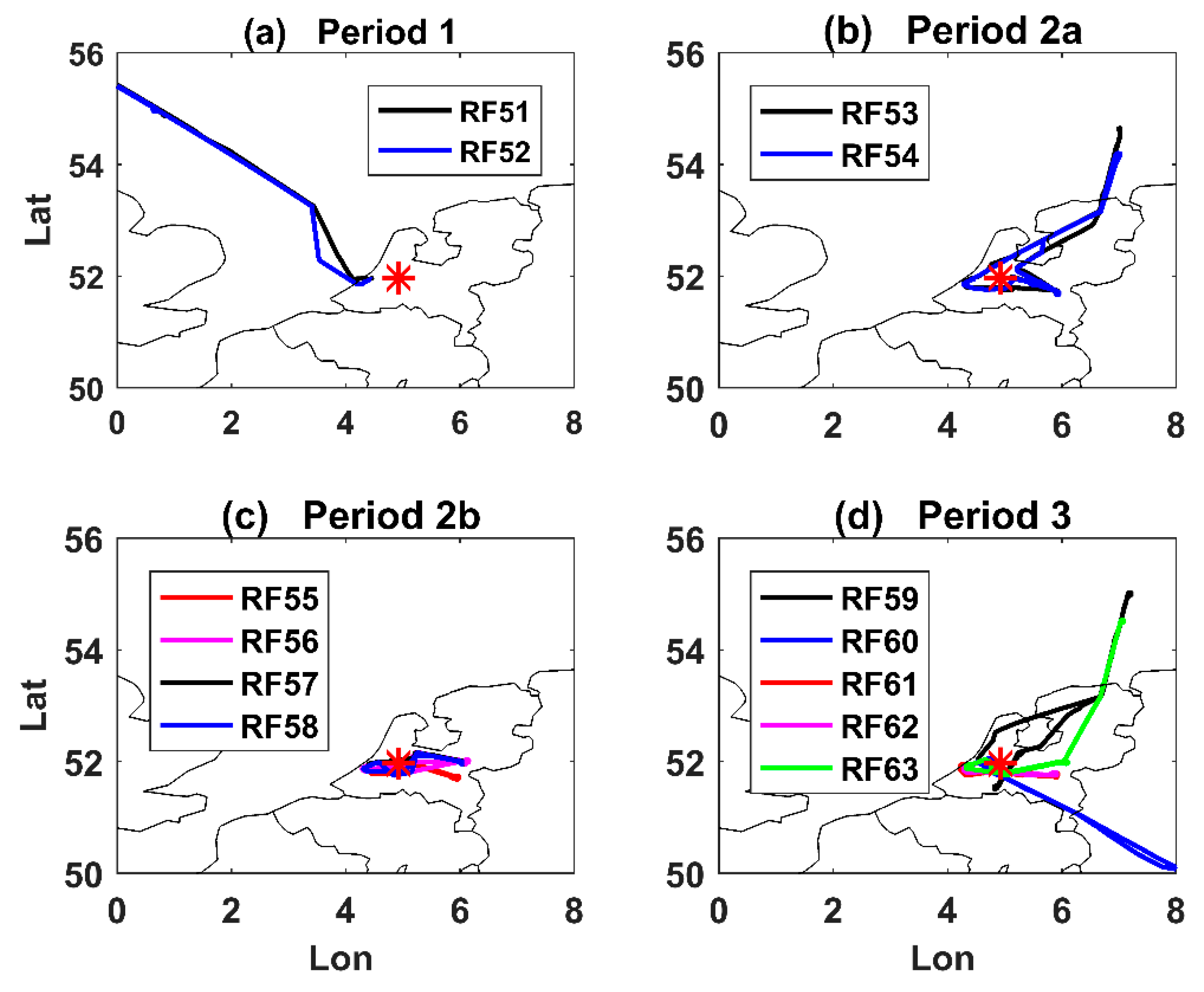Figure 4 shows the comparison between the predicted and observed vertical profiles of SO₄, NO₃, NH₄ and OM concentration, during the period 1, 2a, 2b, and 3, respectively. Modelled data have been extracted interpolating the output point by point along the flight trajectories. In Figure 4, the dots represent the TMs and the bars denote the 25th and 75th percentiles of observed and modelled distributions. For comparisons, the observed and modelled profiles have been projected on 16 layers of 250 m depth.

During P1, WRF-CHIMERE captures the profile of observed mass concentration in the marine PBL, except for SO₄ that is underestimated by more than a factor of 2 close to the surface. Moreover, during P1, the model exhibits a considerable underestimation above the Planetary Boundary Layer (PBL). Measurements above the PBL during P1 reported in this study are not representative of clean marine air, because they were mainly carried out close to the Dutch coast. The bias above the PBL is most probably due to errors in the wind simulation since the simulated plume is localized further to the South compared to observations (not shown).

During P2a and P2b, the model tends to underestimate the mass concentration of observed SO₄, NO₃, NH₄ and OM especially close to the surface. Moreover, WRF-CHIMERE does not reproduce the observed variability especially during the period 2a. The best agreement between observations and model results was found during P3. During this period, modelled values are within the observed range except for the layers close to the surface. WRF-CHIMERE captures several features of observed vertical shape. Both observed and modelled aerosols increase in the PBL, reach the maximum at an altitude of about 500 m, and show a homogeneous profile above the PBL.

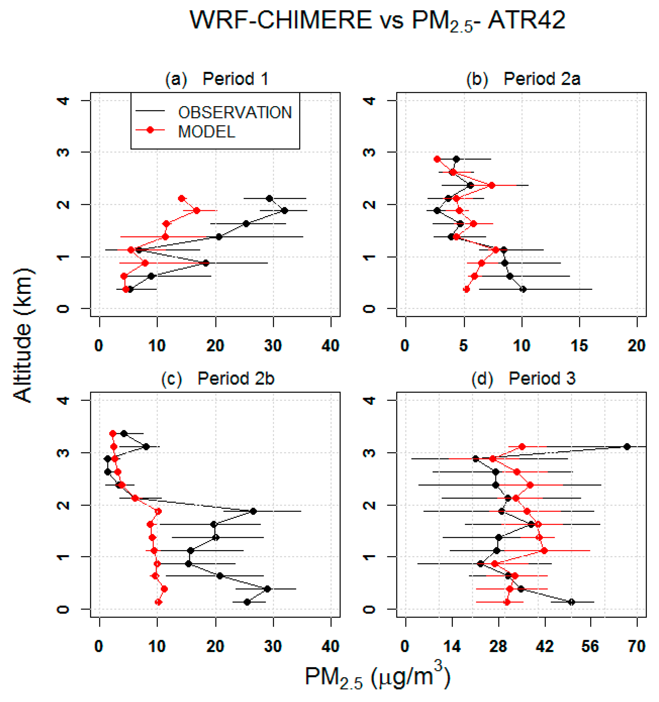
Figure 5 shows the comparison between the observed and predicted vertical profile of PM_2.5. During P1, PM_2.5 is within the observed range in the PBL but is underestimated by a factor 2–3 in the Free Troposphere (FT). The comparison with the flights carried out during the scavenging period (P2a and P2b) shows that the modelled PM_2.5 in the PBL is at the lower end of the observed distribution, but the agreement is satisfying in the FT. Finally, during P3, WRF-CHIMERE underestimates the PM_2.5 mass concentration less than a factor 2 close to the surface, while PM_2.5 is overestimated on the rest of vertical profile. The positive bias in the FT is most likely attributable to the fine fraction of advected desert dust during P3. The overestimation of the dust fine fraction is consistent with the results reported by Menut et al. [84].

Table 5. Trimean (TM) values and interquantile range (IQR) of the aerosol mass concentration of SO₄, NO₃, NH₄, OM, and PM_2.5 measured aboard the ATR-42 and simulated by WRF-CHIMERE. The values are calculated over the whole periods analysed in boundary layer (PBL) and free troposphere (FT). The units are in µg/m³.

	PBL		FT
	TM (IQR)		TM (IQR)
Species	OBS	MOD	OBS	MOD
SO4	2.5 (2.5)	1.4 (1.7)	2.4 (2.9)	1.1 (1.2)
NO3	1.9 (5.1)	2.4 (4.3)	0.2 (0.4)	1.1 (2.9)
NH4	1.8 (3.0)	1.1 (1.3)	1.0 (1.1)	0.7 (1.1)
OM	3.7 (6.1)	1.5 (2.4)	2.3 (3.4)	1.1 (1.8)
PM2.5	19 (23)	13 (15)	15 (33)	16 (28)

summarizes the statistical indices related to the comparison between predicted and observed aerosol mass concentration over the whole campaign in the PBL and FT. WRF-CHIMERE underestimates the TM of SO₄ on average by about 1.1 µg/m³ (or −50%) in both PBL and FT. By contrast, NO₃ TM is overestimated by 0.5 (+26%) and 0.9 µg/m³ (+450%) in the PBL and FT, respectively. However, looking at Figure 4, we underline that this bias is essentially due to P2a period and therefore does not reflect a systematic error of the model in aerosol nitrate simulation. Particulate ammonium is simulated within a factor 2 with respect to the observations, the bias is −39% and −30% in the PBL and FT, respectively. OM is systematically underestimated by a factor 2–3 in both PBL and FT. Average PM_2.5 is underpredicted by the model by −6 µg/m³ (−32%) in the PBL, but shows a negligible error (+7%) in the FT. The analysis of IQR reveals the general tendency of the model to underestimate the variability of aerosol mass concentration found in the observations, except for NO₃ and NH₄ in the PBL and FT respectively. The underestimation of the aerosol mass concentration variability is a common feature found in other modeling systems (e.g., Tuccella et al. [76]). Part of the model underestimation during P2a and P2b could be related to an excess of wet scavenging in The underestimation of the aerosol mass concentration variability is a common feature found in other modeling systems (e.g., Tuccella et al. [76]). Part of the model underestimation during P2a and P2b could be related to an excess of wet scavenging in the model. Another critical factor for a correct simulation of bulk aerosol mass is a proper simulation of the aerosol size distribution. This will be discussed in the Section 4.5.2.

4.5.2. Aerosol Size Distribution and CCN

The first step for reliable simulations of ACI is a satisfactory prediction of the aerosol size number distribution together with a proper representation of aerosol mass and composition. These three elements control the number of aerosol particles activated as cloud droplet.

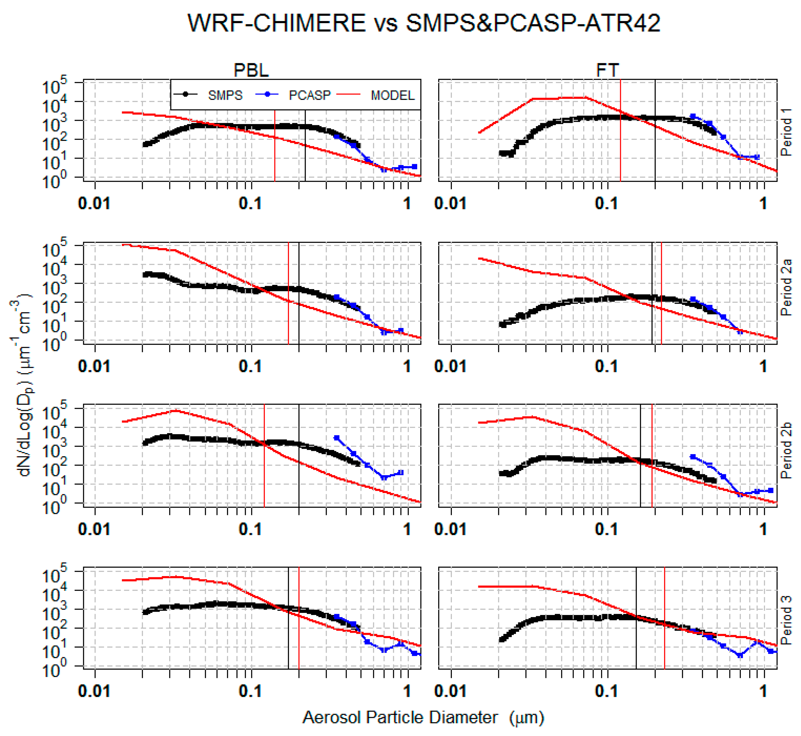
Figure 6 shows the TMs of aerosol size distribution simulated and observed aboard the ATR-42 in all three periods within the PBL and FT. WRF-CHIMERE exhibits a larger number of aerosol particles in the Aitken mode with respect to the observations in both PBL and FT during P1, P2, and P3. CHIMERE particles relative to the bins of Aitken mode (aerosol particle with diameter between 0.01 and 0.1 µm) are overestimated from a few hundred up to 2–3 orders of magnitude.

There is also a tendency to underestimate the larger particles of the accumulation mode. These results suggest that the overestimation of ultrafine particles is likely related to an excess of particle formation from nucleation. Moreover, the lack of sufficient particles in the accumulation mode reduces the coagulation of ultrafine aerosols on larger existing particles, so that the loss of smaller particles by coagulation is not efficient enough. Another probable source of error is the size distribution at emission: a profile is applied to the total mass of primary aerosol emissions into the model bins (fixed for each type of source and the emitted species). CHIMERE does not include a prognostic treatment of particle number, which is diagnosed from the mass, density and particle diameter. It should be noted that ACI is unlikely affected by ultrafine particles, the most favoured particles to act as CCN are those larger than 100 nm. Therefore, it is interesting to explore how the model reproduces these particles referred to as condensation nuclei (CN) in this study.

Table 6. Trimean values of condensation nuclei (CN) cloud condensation nuclei (CCN) concentration, cloud, a6rosol hygroscopicity, critical diameter, and condensation nuclei efficiency (CCNE) measured aboard the ATR-42 and simulated by WRF-CHIMERE. The values are calculated in each period analyzed in boundary layer (PBL) and free troposphere.

	P1				P2a				P2b				P3
	PBL		FT		PBL		FT		PBL		FT		PBL		FT
	OBS	MOD	OBS	MOD	OBS	MOD	OBS	MOD	OBS	MOD	OBS	MOD	OBS	MOD	OBS	MOD
CN	531	192	1831	2701	551	429	229	300	1520	1457	176	591	1303	2561	342	879
CCN	86	115	886	1409	181	119	110	68	627	604	160	47	463	484	190	99
CD	0.22	0.14	0.20	0.27	0.20	0.17	0.19	0.22	0.20	0.12	0.16	0.19	0.17	0.20	0.15	0.23
CCNE	38	58	48	12	34	27	46	15	38	44	53	23	38	19	58	12

reports the observed and predicted TMs of CN within the PBL and FT. CN are underpredicted in the PBL from a factor 2.8 during P1 to negligible bias during P2a and P2b. By contrast, WRF-CHIMERE predicts a larger number of CN (about a factor 2) in the PBL during the large transport days when a significant contribution to CN is given by the fine fraction of the dust advected from the desert. In the FT, the model exhibits a systematic positive bias ranging from a factor 1.3 up to 3.3. Looking at Figure 6, it should be observed that the bias in simulating CN is not uniformly distributed with the aerosol diameter but in both case of low and high bias, the model in general overestimates the CN with diameter between 0.1 and 0.2 µm and underestimates the particles larger than 0.2 µm. This bias could have an important impact on the CCN calculation leading to larger (lower) concentrations at high (low) levels of supersaturation.

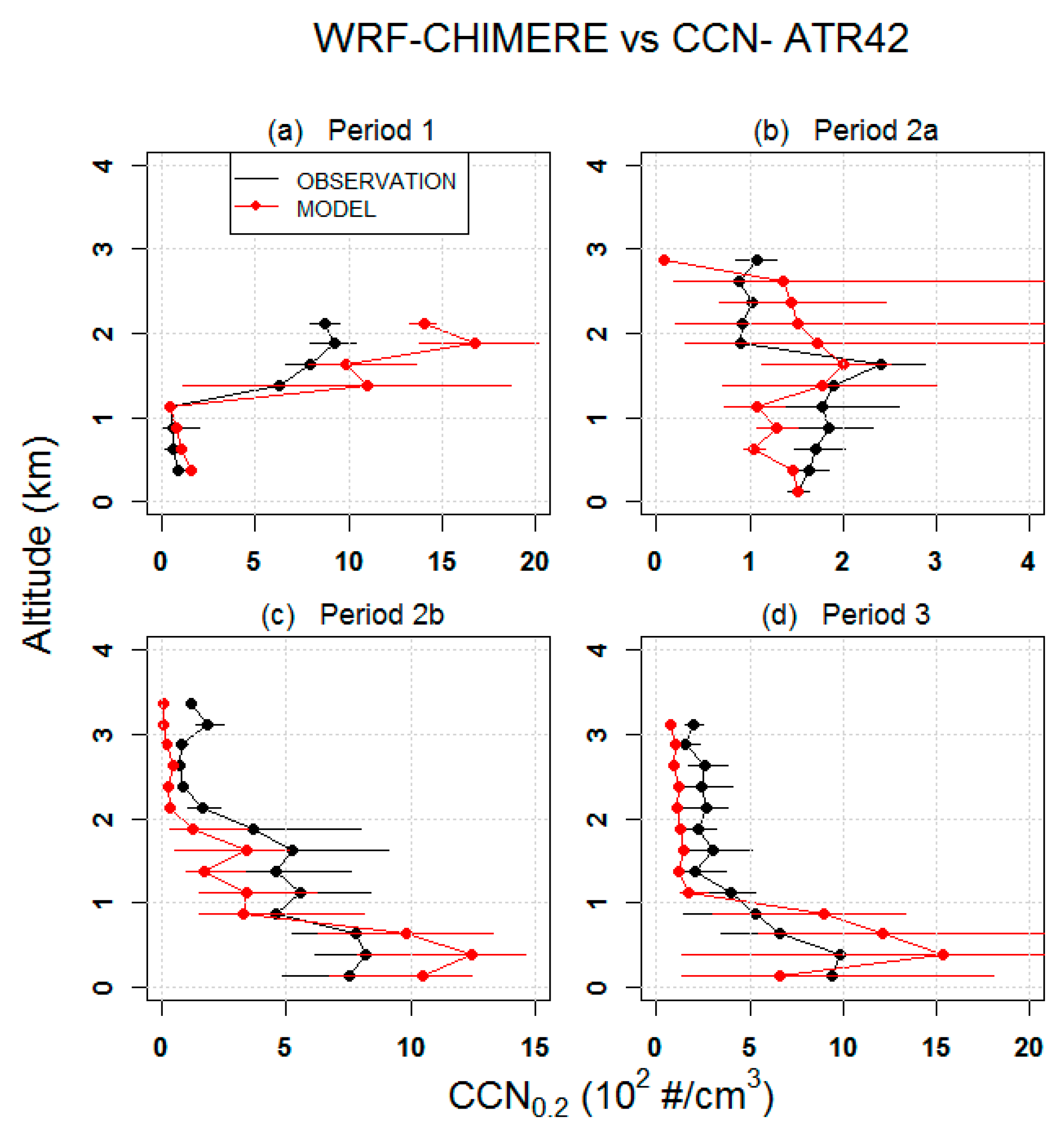
Vertical profiles of CCN at 0.2% of supersaturation are shown in Figure 7 and their TMs for each period are reported in Table 6. In the PBL, CCN concentration is underestimated during wet scavenging days and overestimated during P1 and P3, but the bias is always lower than a factor 1.5. Concerning the FT, although CN are high biased in each period, modelled CCN are lower relative to the observations by a factor 3.4 during P2b, 1.6 during P2a and P3, respectively. CCN are overestimated in the FT only during P1. The results found here are comparable with the performances of other state-of-art models. For example, Tuccella et al. [76] comparing WRF/Chem to our same data set, reported an overestimation of CCN by a factor 1.5 in the mixed layer and a small bias in the FT.

In addition to the size distribution, modelled CCN bias is associated with the critical diameter (CD) and aerosol composition. CD is defined as the cut-off diameter above which all particles act as CCN at a given level of supersaturation. Observed CD has been calculated from aerosol size number distribution and CCN measurements. It is given by the diameter at which the integrated size distribution equals the CCN concentration. TMs of observed and predicted CD are reported in Table 6 and are overlaid to the size distributions shown in Figure 6. To explain the link between aerosol size distribution, CD and composition in reproducing CCN, we focus as an example on the results obtained in the FT during P3. We choose this case because, as shown in Figure 6, the predicted size distribution is very similar to the observations for diameters larger than about 0.15 µm, therefore the CCN bias has a negligible dependence on the size distribution. In the case examined, CD is larger than the observed one by a factor 1.5, explaining the negative bias of CCN despite the reasonable simulation of the size distribution (for diameters larger than 0.15 µm). According to Kohler theory, CD depends on the aerosol hygroscopicity that in turn is a function of composition. Given a supersaturation level, the larger the hygroscopicity, the lower the CD. As a consequence, underestimation of hygroscopicity in the FT during P3 is most likely due to an excess of dust in the fine fraction of modelled PM_2.5 (see Section 4.5.1) combined with the missing of sufficient inorganic (sulphate, ammonium, nitrate) mass concentration (about 50% less compared to AMS data) that lowers the aerosol solubility. A measure of hygroscopicity is given by CCN efficiency (CCNE) defined as the ratio between CCN and CN. The observed and modelled values are shown in Table 6. As expected, CCNE simulated by WRF-CHIMERE for the case examined is about 5 times smaller than the observations. In the PBL, CCNE is simulated within a factor 2 but the error is larger the FT.

4.5.3. Cloud Optical Properties

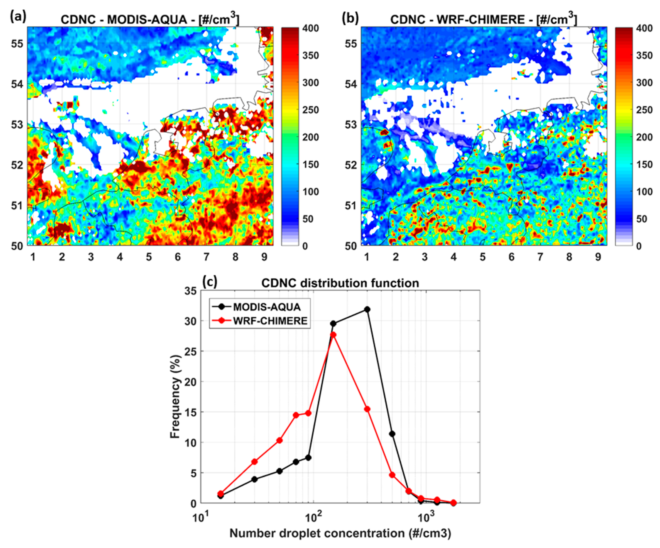
Figure 8a,b show the TMs of cloud droplet concentration number (CDNC) averaged over the whole period (14–30 May 2008). Satellite CDNC has been calculated starting from liquid cloud droplet effective radius (Re) and liquid cloud optical depth (LCOD) following the method used by Georg and Wood [85]. WRF-CHIMERE captures qualitatively several features of the spatial distribution of observed CDNC. The gradient between North Sea and land is reproduced by model, as well as the distribution of the maxima values of CDNC, with the exception of some regions where the model shows an important bias, for example South-East of England coast, in the middle of the border between the Netherlands and Germany, on the border between France and Belgium. As shown in

Table 7. Domain trimean (TM) values and interquantile range (IQR) of observed and modelled cloud droplet number concentration (CDNC), droplet effective radius (Re), liquid cloud optical depth (LCOD), and ice cloud optical depth (ICOD).

	MODIS	WRF-CHIMERE
	TM (IQR)	TM (IQR)
CDNC (#/cm3)	194 (213)	116 (123)
Re (µm)	9.3 (3.8)	9.2 (3.7)
LCOD	16 (15)	12 (20)
ICOD	14 (19)	7 (18)

, domain average of calculated CDNC is underestimated by 40%.

As it is evident from Figure 8a,b, both model and observations show a fine scale variability that makes a point-by-point comparison between WRF-CHIMERE and MODIS difficult. Modelled and observed clouds exhibit small differences in location and timing of formation. As a consequence, the distribution function (DF) is a useful tool that provides an overall view of WRF-CHIMERE performance in reproducing CDNC and at the same time is independent by spatial and temporal phase errors [86]. Observed and modelled DFs of CDNC are shown in Figure 8c.

In general, WRF-CHIMERE overestimates the occurrence frequency (OF) of CDNC less than 100 #/cm³ and underpredicts the largest values. Specifically, the cumulated OF of CDNC representative of “clean atmospheres” (less than 100 #/cm³) are overestimated by a factor of 2. By contrast, modelled CDNC typical of “polluted conditions” (100–600 #/cm³) are about 1.5 times smaller relative to the MODIS data, while values representative of “very polluted conditions” (larger than 600 #/cm³) constitute the 0.5% and 1.5% of observed and modelled sample, respectively.

The origin of the bias of modelled CDNC is related to the uncertainties in aerosol size distribution and hygroscopicity prediction. As already mentioned in the Section 4.5, CCN are underestimated at low supersaturations and high biased for large supersaturations, because modelled CN are larger than observations at the smallest diameters of accumulation mode (0.1–0.2 µm) but are low biased for larger sizes. Therefore, given that the range of supersaturation of our simulations is relatively low, the main uncertainties in prediction of CDNC is due to the general underestimation of CN at larger diameter of aerosol size distribution. Another factor that explains CDNC bias is the uncertainty related to hygroscopitcity that in turn affects the CD. As discussed in the previous Section, modelled CD is larger with respect to the observed one because CCNE (which is a measure of aerosol hygroscopitcity) predicted by WRF-CHIMERE is low relative to ATR-42 data. Larger CD implies a lower amount of CCN that may be activated as cloud droplet.

Figure 9a,b shows the TMs calculated over the whole period of liquid cloud droplet effective radius (R_e). As for CDNC, WRF-CHIMERE is able to reproduce qualitatively the features of observed Re pattern. The gradient between North Sea and land and the distribution of the maxima values of Re are reproduced by the model, with the exception of the regions where a bias in CDNC. In these regions, CDNC was noticed and Re are anticorrelated. As shown in Table 7, modelled and measured TM and IQR of R_e show very similar values, meaning that WRF-CHIMERE is able to capture the central tendency of measured R_e.

As displayed in Figure 9c, the maximum of DF of modelled R_e has the peak shifted toward larger values with respect to satellite data. DFs of MODIS and WRF-CHIMERE exhibit the maximum around 9–10 and 7–8 µm, respectively. Cumulated OF around the observed maximum (6–9 µm) represents about the 50% of MODIS sample, while in the same range falls the 34% of WRF-CHIMERE data. The shift of the peak toward larger droplet found in WRF-CHIMERE is a consequence of low CDNC in the model.

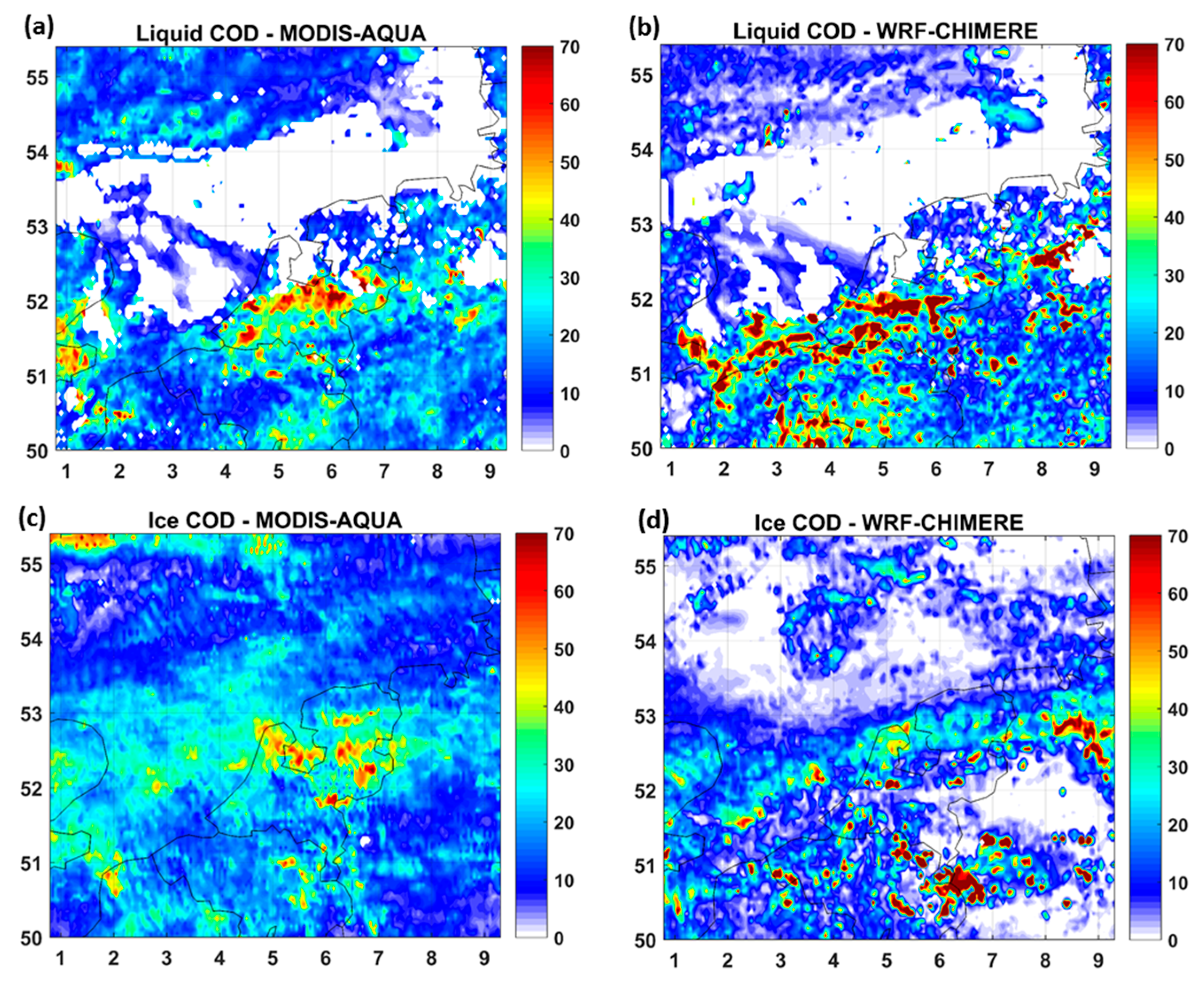
Figure 10a,b report the TMs of retrieved and predicted LCOD, respectively. As for previous variables, WRF-CHIMERE explains the features of LCOD observed by MODIS. It reproduces the lowest values of the pattern observed in the North of the domain, and the band of maximum values extending from northern France up to northwest Germany crossing Belgium and The Netherland. WRF-CHIMERE overestimates observed LCOD along this band, but the model tends to slightly underpredict LCOD elsewhere. LCOD averaged over the domain is reported in Table 7. It is underestimated by a factor 1.3 (−19%) but exhibits larger variability (IQR) than the observations.

As we would expect, the bias in simulation of cloud optical properties depend on the particular aerosol mechanism adopted in the models. For example, Tuccella et al. [76], using WRF/Chem with a modal aerosol model on the same region and period of our study, found an opposite behavior with respect to our results. Indeed, Tuccella et al. [76] reported an overestimation of CCN that produces smaller Re and larger LCOD relative to the observations. However, it should be noted that the magnitude of bias found here is comparable to WRF/Chem performances shown by Tuccella et al. [76], for example LCOD is overestimated by a few percent up to 48%.

As described in Section 2, WRF-CHIMERE includes also the glaciation indirect effect through the processes of heterogeneous and homogeneous ice nucleation starting from aerosol predicted by chemical modules. Unfortunately, no available in situ measurements allow the evaluation of the ice particle concentration. The simulated ice cloud optical depth (ICOD) was compared to that observed by MODIS, including the precipitating hydrometeors and suspended ice cloud.

Figure 10c,d shows the TMs of observed and simulated ICOD. WRF-CHIMERE captures qualitatively the maximum values displayed in the observed pattern in a band between 52–53° N and on the border between Belgium and Germany. WRF-CHIMERE tends to underpredict the minimum values of ICOD observed over the sea and Northwestern Germany. Simulated ICOD TM average is about half that of observations, but IQRs are very similar meaning larger dispersion of modelled values with respect to MODIS. 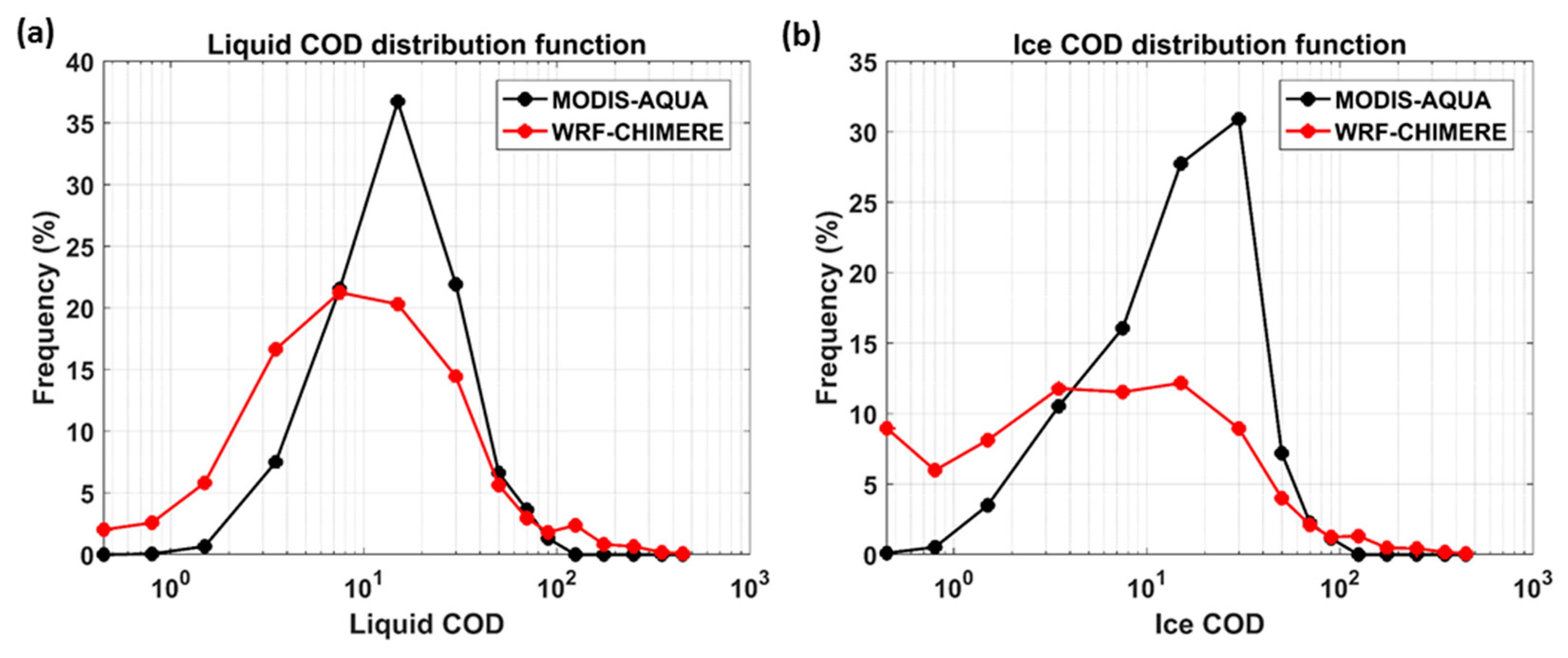Figure 11b reports the comparison between observed and modelled ICOD DFs. The comparison suggests that WRF-CHIMERE has about 15% more of ICOD less than 2. DFs reach maximum for values between 3–20 and 20–40 for observed and predicted sample, respectively. WRF-CHIMERE underestimate the maximum of observed OF by about 15–20%.

Although in this section we have focused on the relationship among aerosol size distribution, hygroscopicity, CDNC, and COD, the uncertainties in simulating cloud optical properties may be also related to model setup used. For example, Barò et al. [87] investigated the sensitivity of WRF/Chem of ACI to two different cloud microphysics schemes, and found serious differences in CDNC and cloud water mixing ratio patterns predicted by two parameterizations that depend on geographical location, pollution level, and season. In addition to cloud microphysics representation, Otkin and Greewald [85] showed an important sensitivity of cloud optical properties to PBL schemes.

5. Sensitivity Test

In this section, as first example of application of WRF-CHIMERE model including ACI, we discuss the regional response to aerosol emission abatement. The studies of global warming mitigation strategies are usually conducted focusing only the reduction of emissions of aerosol species that cause the warming of the atmosphere such as the black carbon [28]. On a practical level, it is not easy to reduce the emission of single species since it is co-emitted together to other SLCPs and precursor gases that lead to secondary aerosol formation. For this reason, we did not focus on a single aerosol species, but we have reduced both primary aerosols and precursor gases emissions from all anthropogenic sources. Specifically, the method described in Section 3 was used but with anthropogenic emission fluxes halved in all three domains. Our test should be intended as a limit case of emission abatement. Aerosol direct effect is not included in the simulations. Moreover, chemical boundary conditions for D1 remain unchanged in our test. As a consequence, the effect induced by emission reduction could be underestimated. It is should be also noticed that given the short period of interest, the test is not a climatic simulation. The test is only dedicated to short-term indirect effects of aerosols on radiation, clouds, temperature and precipitations.

To investigate the change on the radiation budget due to emission reduction via indirect effects, we define the indirect radiative effect (IRE) as the average difference in the net radiation flux (down–up) at surface between sensitivity test and reference run including all current anthropogenic sources. Domain average effect of emission reduction on CCN concentration, radiation flux, and temperature is reported in

Table 8. Domain average effect of anthropogenic emission reduction. The effect on CCN and temperature is calculated as the difference between the perturbed and reference run. Indirect radiative effect (IRE) is the difference in the net radiation flux (down-up) at surface between sensitivity and perturbed simulation.

	Land	Sea	Land + Sea
CCN0.2 (#/cm3)	−496 (−65%)	−284 (−58%)	−386 (−62%)
SW IRE (W/m2)	+1.56	+0.27	+0.89
LW IRE (W/m2)	−0.24	+0.41	+0.10
SW+LW IRE (W/m2)	+1.32	+0.68	+0.99

.

According to WRF-CHIMERE, halving of anthropogenic emissions reduces PBL average concentration of CCN at 0.2% of supersaturation by about 60%. The decrease of 60% of CCN concentration against the 50% of emission highlights the non-linear behavior of CCN formation. Figure 12 shows the average IRE calculated over the whole period (14–30 May 2008) for shortwave (SW), longwave (LW), and total radiation. Average IRE radiative effect on SW radiation is positive over whole domain and is equal to +0.89 W/m². This result is consistent with our expectations. Lower CCN number concentration implies lower CDNC with larger diameter with respect to reference simulation, and thus less efficient clouds in reflecting the incoming solar radiation. Although SW IRE is positive on average, its distribution is not homogeneous on the domain but appears “noisy”, locally IRE may reach values of ±12 W/m². This suggests that emission abatement influences timing and location of cloud formation. Beside average IRE is different between land and sea. We notice that the amplitude of IRE is +1.56 and +0.27 W/m² on the land and sea respectively. On the sea, we note some regions where IRE is mainly positive.

LW IRE is also positive (+0.10 W/m²) but its magnitude is less than change of SW radiation budget (about 11%). As shown in Figure 12b, LW IRE displays a marked asymmetry between land and sea. It is positive on the sea (+0.41 W/m²) and negative on land (−0.24 W/m²). Given the non-linearity of the aerosol-cloud-radiation system, it is not easy to explain this asymmetry. A possible explanation is related to liquid cloud top height (CTH) change that results from emission reduction.

Figure 13 shows the cumulative distribution frequency of liquid CTH simulated by WRF-CHIMERE in the reference run separately for land and sea. In Figure 13 is also shown the average change in CTH for low (100 < CTH < 800 m), middle (800 < CTH < 1500 m), and high (CTH > 1500 m) liquid clouds. As we may infer from Figure 13, 80% of sea clouds is constituted by clouds with top lower than 1500, while on the land these are less than 50% of the sample. According to the model, when the anthropogenic emissions are halved, we note that top height of low and middle liquid clouds tends to increase, at the same time the top of high cloud lowers. Therefore, being the scenario on the sea dominated by low and middle cloud, the increase of their top decreases the outgoing longwave radiation. By contrast on the land where high clouds are much more frequent, the lowering of their top increase the flux of the outgoing longwave radiation. As a result, on the land SW IRE is partially compensated by LW IRE giving a net value of +1.32 W/m². On the sea, SW and LW IRE have the same sign and net IRE is +0.68 W/m². Domain average of IRE is +0.99 W/m².

The effect induced by emissions reduction on temperature at 2 m (T2) and precipitation rate is mainly representative of local changes. Instantaneous changes of T2 locally may reach values of ±7°C, while the instantaneous changes of precipitation rate are up to ±50 mm/day.

Error associated with IRE is mainly due to the uncertainties in CDNC simulation. Model evaluation has shown the model tendency to underestimate CDNC leading to larger cloud effective radius and lower cloud optical thickness with respect to the observations. As a consequence, we have to expect less incoming radiation reflected to the space by clouds (lower cloud radiative forcing) in the reference run. When CDNC is reduced in the sensitivity test, we would expect a larger warming effect compared to the one we would have in the real atmosphere, if the droplets are reduced by the same amount. Our IRE has been estimated to be overestimated by about 10%. The method used to calculate the uncertainty is reported in the Appendix B.

6. Conclusions

Aerosol indirect effects have been implemented within the online version of WRF-CHIMERE coupled model [25]. In this work, we have extended the two-way coupling to the feedback from the aerosol-cloud interaction. First, second and glaciation indirect effects have been included in the model via the cloud microphysics scheme of Thompson and Eidhammer [40]. Aerosol activation as cloud droplets, heterogeneous and homogeneous ice nucleation are calculated starting from aerosol size distribution predicted by CHIMERE model.

WRF-CHIMERE with indirect effects has been evaluated in the period 14–30 May 2008 comparing cloud resolving simulations (4 km) with ground-based, aircraft measurements of aerosol mass and particle collected on the Benelux Union during the EUCAARI campaign [35] and MODIS cloud data. During the studied period, the atmospheric conditions were characterized by alternation of relative stable weather conditions, wet scavenging days, and days with long-range transport of dust from Sahara desert.

WRF-CHIMERE captures the day-to-day variations of aerosol mass concentrations at surface. Observed SO₄, NO₃, NH₄, OM, PM_2.5, and PM₁₀ are reproduced with correlation coefficients larger than 0.50. The analysis of the bias reveals that the model tends to overestimates the observed ammonium nitrate at ground stations and underestimates OM. Comparison between model and observed aircraft profiles shows that WRF-CHIMERE is able to reproduce the vertical profiles of SO₄, NO₃, NH₄, OM, and PM_2.5, but their mass concentration is underestimated in the model especially in the PBL during wet scavenging days, suggesting an excess of wet deposition. By contrast, OM is underestimated over the whole period by about a factor 2. PM_2.5 is overpredicted above the surface during the long range transport days, most likely because of an excesses of fine dust.

Model evaluation with aerosol size number distribution measured aboard the ATR-42 shows the systematic tendency of WRF-CHIMERE to overpredicted the particles of the Aitken mode in both PBL and free troposphere. Simulation of condensation nuclei (CN) (particles larger than 100 nm) does not show a systematic bias in the PBL, bias sign changes with the synoptic frame. By contrast, CN in the FT are overpredicted from a factor 1.3 up to 3.3. However, the bias in simulating CN is not uniformly distributed with the aerosol diameter but the model overestimates the CN with diameter between 0.1 and 0.2 μm and underestimates the particles larger than 0.2 µm.

Despite the uncertainties in aerosol size distribution simulation, predicted CCN vertical profiles have a good degree of similarity with the observed one. In the PBL, modelled CCN concentration is within a factor 2 with respect to the observations. Concerning the FT, although CN are high biased over the whole period, simulated CCN does not show a systematic bias, but this varies with the evolution of synoptic configuration. This behavior is explained looking at the modelled critical diameter (CD) and aerosol hygroscopicity. Taking a case where the predicted size distribution has a negligible bias with respect to the observations as for example in the FT during dust transport days, we have found that CCN efficiency (a measure of aerosol hygroscopicity defined as the ratio between CCN and CN concentrations) is 5 times smaller with respect the observations. This implies a larger CD in the model with a consequent underestimation of CCN. CCN efficiency bias is related to the uncertainties in simulating aerosol mass. In the case examined during the long range dust transport days, is most likely due to an excess of dust (hydrophobic) in the fine fraction of modelled PM_2.5 combined with the missing of sufficient inorganic salt mass (hydrophilic).

WRF-CHIMERE skill in reproducing cloud optical properties has been evaluated comparing the model results with MODIS L2 cloud products. WRF-CHIMERE reproduces several features of the average pattern of observed cloud droplet number concentration (CDNC). The cumulated observed distribution frequencies of CDNC less than 100 #/cm³ are overestimated by a factor 2. By contrast, modelled CDNC in the range of 100–600 #/cm³ are about 1.5 times smaller relative to the MODIS data. As for CDNC, WRF-CHIMERE is able to reproduce the average spatial distribution of observed liquid cloud effective radius (R_e) pattern. The analysis of Re distribution frequencies suggest that our model has the pick shifted toward larger values with respect to satellite data and at the same time there is a certain tendency in the model to overestimate the frequency of the smallest droplets (R_e < 6 µm). Modelled average domain of liquid cloud optical depth (LCOD) is underestimated by 19% with respect to MODIS data.

The results discussed in this work indicate that the new functionality implemented in the model is able to reproduce the observations in a spatial and temporal scale dominated by high meteorological, chemical and emission variability. Compared to other similar modelling systems, results are in the same order of magnitude (although other models are never completely similar) and represent the current state of the art in regional chemistry-transport modelling. Therefore, our modeling system is suitable to be used in studies involving the feedback between aerosol and clouds. As first example of application, we have discussed the results of a sensitivity simulation where the anthropogenic emissions have been halved. The impact of emission abatement has been quantified through the indirect radiative effect (IRE) defined as the average difference in the net radiation flux (down–up) at surface between sensitivity test and reference run including all current anthropogenic sources. Average IRE on the cloud resolving domain is positive for both short and long wave radiation.

A closer inspection to the regional distribution of IRE has revealed that the change of long wave radiation budget is negative on the land and positive on the sea. This asymmetry is explainable with the change of cloud top height (CTH). The analysis of the frequency distribution of liquid CTH in the reference run has shown that cloud coverage on the sea is dominated by low (100 < CTH < 800 m) and middle (800 < CTH < 1500 m) clouds, while high clouds (CTH > 1500 m) dominate on the land. According to the model, halving of anthropogenic emissions increases the top height of low and middle liquid clouds and lowers the top of highest clouds. Therefore, on the sea the increase of low and middle CTH decreases the outgoing longwave radiation flux. By contrast on the land where high clouds are much more frequent, the lowering of their top increases the flux of the outgoing longwave radiation.

The effects induced by halving of anthropogenic emissions have been also investigated in terms of surface temperature and precipitation rate changes. Model results have shown that there are important instantaneous changes at local scale (up to ±6°C for maximum and minimum temperatures, ±50 mm/day for precipitation). In the framework of regional air quality modelling, this could have a large impact on isolated pollutants plumes during their transport.

Although the results obtained in this work are encouraging and show that WRF-CHIMERE performances are comparable with other state-of-the-art online modeling systems, there is still much room for further evaluations and improvements. In our work WRF-CHIMERE evaluation is limited to the liquid water cloud, further verification with observations from cirrus cloud fields are recommended. Model comparison with CCN aircraft measurements and MODIS cloud data have highlighted that the uncertainties in simulating ACI in WRF-CHIMERE model manly arises from error in prediction of aerosol size number distribution and composition. For this reason, ACI simulation could improve updating aerosol model with the recently introduced scheme of Couvidat et al. [88]. Finally, ACI simulations with current version of WRF-CHIMERE are recommended with horizontal resolution less than 10 km because the indirect effect is considered only for grid-scale clouds. The extension of ACI to parameterized (convective) clouds is desirable and could be done through some aerosol aware convective parameterizations implemented in WRF like that of Grell and Freitas [54] or Berg et al. [89]. This development would allow simulating ACI at resolution coarser than cloud resolving scale.

References

1. Boucher, O.; Randall, D.; Artaxo, P.; Bretherton, C.; Feingold, G.; Forster, P.; Kerminen, V.-M.; Kondo, Y.; Liao, H.; Lohmann, U.; et al. Clouds and Aerosols. In Climate Change 2013: The Physical Science Basis. Contribution of Working Group I to the Fifth Assessment Report of the Intergovernmental Panel on Climate Change; Stocker, T.F., Qin, D., Plattner, G.-K., Tignor, M., Allen, S.K., Boschung, J., Nauels, A., Xia, Y., Bex, V., Midgley, P.M., Eds.; Cambridge University Press: Cambridge, UK; New York, NY, USA, 2013. [Google Scholar]
2. Hansen, J.; Sato, M.; Ruedy, R. Radiative forcing and climate response. J. Geophys. Res. Atmos. 1997, 102, 6831–6864. [Google Scholar] [CrossRef] [Green Version]
3. Haywood, J.; Boucher, O. Estimates of the direct and indirect aerosol radiative forcing due to tropospheric aerosols: A review. Rev. Geophys. 2000, 38, 513–543. [Google Scholar] [CrossRef]
4. Lohmann, U.; Feichter, J. Global indirect aerosol effects: A review. Atmos. Chem. Phys. 2005, 5, 715–737. [Google Scholar] [CrossRef]
5. Twomey, S.A. Pollution and planetary albedo. Atmos. Environ. 1974, 8, 1251–1256. [Google Scholar] [CrossRef]
6. Twomey, S.A. The influence of pollution on the shortwave albedo of clouds. J. Atmos. Sci. 1997, 34, 1149–1152. [Google Scholar] [CrossRef]
7. Albrecht, B. Aerosols, cloud microphysics, and fractional cloudiness. Science 1989, 245, 1227–1230. [Google Scholar] [CrossRef] [PubMed]
8. Rosenfeld, D.; Lohmann, U.; Raga, G.B.; O’Dowd, C.D.; Kulmala, M.; Fuzzi, S.; Reissel, A.; Andreae, M.O. Flood or Drought: How do aerosols affect precipitation? Science 2008, 321, 1308–1313. [Google Scholar] [CrossRef] [PubMed]
9. Small, J.D.; Chuang, P.Y.; Feingold, G.; Jiang, H. Can aerosol decrease cloud lifetime? Geophys. Res. Lett. 2009, 36, L16806. [Google Scholar] [CrossRef]
10. Forster, P.; Ramaswamy, V.; Artaxo, P.; Berntsen, T.; Betts, R.; Fahey, D.W.; Haywood, J.; Lean, J.; Lowe, D.C.; Myhre, G.; et al. Changes in Atmospheric Constituents and in Radiative Forcing. In Climate Change 2007: The Physical Science Basis. Contribution of Working Group I to the Fourth Assessment Report of the Intergovernmental Panel on Climate Change; Solomon, S., Qin, D., Manning, M., Chen, Z., Marquis, M., Averyt, K.B., Tignor, M., Miller, H.L., Eds.; Cambridge University Press: Cambridge, UK; New York, NY, USA, 2007. [Google Scholar]
11. DeMott, P.J.; Prenni, A.J.; Liu, X.; Kreidenweis, S.M.; Petters, M.D.; Twohy, C.H.; Richardson, M.S.; Eidhammer, T.; Rogers, D.C. Predicting global atmospheric ice nuclei distributions and their impacts on climate. PNAS 2010, 107, 11217–11222. [Google Scholar] [CrossRef] [PubMed] [Green Version]
12. Baklanov, A.; Schlünzen, K.; Suppan, P.; Baldasano, J.; Brunner, D.; Aksoyoglu, S.; Carmichael, G.; Douros, J.; Flemming, J.; Forkel, R.; et al. Online coupled regional meteorology chemistry models in Europe: Current status and prospects. Atmos. Chem. Phys. 2014, 14, 317–398. [Google Scholar] [CrossRef]
13. Huang, Y.; Dickinson, R.E.; Chameides, W.L. Impact of aerosol indirect effect on surface temperature over East Asia. PNAS 2006, 103, 4371–4376. [Google Scholar] [CrossRef] [PubMed] [Green Version]
14. Bangert, M.; Kottmeier, C.; Vogel, B.; Vogel, H. Regional scale effects of the aerosol cloud interaction simulated with an online coupled comprehensive chemistry model. Atmos. Chem. Phys. 2011, 11, 4411–4423. [Google Scholar] [CrossRef] [Green Version]
15. Yang, Q.; Gustafson, W.I., Jr.; Fast, J.D.; Wang, H.; Easter, R.C.; Wang, M.; Ghan, S.J.; Berg, L.K.; Leung, L.R.; Morrison, H. Impact of natural and anthropogenic aerosols on stratocumulus and precipitation in the Southeast Pacific: A regional modelling study using WRF-Chem. Atmos. Chem. Phys. 2012, 12, 8777–8796. [Google Scholar] [CrossRef]
16. Forkel, R.; Balzarini, A.; Baró, R.; Bianconi, R.; Curci, G.; Jiménez-Guerrero, P.; Hirtl, M.; Honzak, L.; Lorenz, C.; Im, U.; et al. Analysis of the WRF-Chem contributions to AQMEII phase2 with respect to aerosol radiative feedbacks on meteorology and pollutant distributions. Atmos. Environ. 2015. [Google Scholar] [CrossRef]
17. Makar, P.A.; Gong, W.; Hogrefe, C.; Zhang, Y.; Curci, G.; Žabkar, R.; Milbrandt, J.; Im, U.; Balzarini, A.; Baró, R.; et al. Feedbacks between air pollution and weather, part 1: Effects on weather. Atmos. Environ. 2015, 115, 442–469. [Google Scholar] [CrossRef]
18. Makar, P.A.; Gong, W.; Hogrefe, C.; Zhang, Y.; Curci, G.; Žabkar, R.; Milbrandt, J.; Im, U.; Balzarini, A.; Baró, R.; et al. Feedbacks between air pollution and weather, part 2: Effects on chemistry. Atmos. Environ. 2015, 115, 630–645. [Google Scholar] [CrossRef]
19. Kong, X.; Forkel, R.; Sokhi, R.S.; Suppan, P.; Baklanov, A.; Gauss, M.; Brunner, D.; Barò, R.; Balzarini, A.; Chemel, C.; et al. Analysis of meteorology–chemistry interactions during air pollution episodes using online coupled models within AQMEII phase-2. Atmos. Environ. 2015, 115, 527–540. [Google Scholar] [CrossRef] [Green Version]
20. Zhang, B.; Wang, Y.; Hao, J. Simulating aerosol–radiation–cloud feedbacks on meteorology and air quality over eastern China under severe haze conditionsin winter. Atmos. Chem. Phys. 2015, 15, 2387–2404. [Google Scholar] [CrossRef] [Green Version]
21. Grell, G.A.; Peckham, S.E.; McKeen, S.; Schmitz, R.; Frost, G.; Skamarock, W.C.; Eder, B. Fully coupled “online” chemistry within the WRF model. Atmos. Environ. 2005, 39, 6957–6975. [Google Scholar] [CrossRef]
22. Baklanov, A.; Korsholm, U.S.; Nuterman, R.; Mahura, A.; Nielsen, K.P.; Sass, B.H.; Rasmussen, A.; Zakey, A.; Kaas, E.; Kurganskiy, A.; et al. Enviro-HIRLAM online integrated meteorology–chemistry modelling system: Strategy, methodology, developments and applications (v7.2). Geosci. Model Dev. 2017, 10, 2971–2999. [Google Scholar] [CrossRef]
23. Kallos, G.; Solomos, S.; Kushta, J. Air quality—Meteorology Interaction Processes in the ICLAMS Modeling System. In Proceedings of the 30th NATO/SPS International Technical Meeting on Air Pollution Modelling and its Application, San Francisco, CA, USA, 18–22 May 2009. [Google Scholar]
24. Briant, R.; Tuccella, P.; Deroubaix, A.; Khvorostyanov, D.; Menut, L.; Mailler, S.; Turquety, S. Aerosol–radiation interaction modelling using online coupling between the WRF 3.7.1 meteorological model and the CHIMERE 2016 chemistry-transport model, through the OASIS3-MCT coupler. Geosci. Model Dev. 2017, 10, 927–944. [Google Scholar] [CrossRef] [Green Version]
25. Schaap, M.; Timmermans, R.M.A.; Roemer, M.; Boersen, G.A.C.; Builtjes, P.J.H.; Sauter, F.J.; Velders, G.J.M.; Beck, J.P. The LOTOS–EUROS model: Description, validation and latest developments. Int. J. Environ. Pollut. 2008, 32, 270–290. [Google Scholar] [CrossRef]
26. Pleim, J.; Young, J.; Wong, D.; Gilliam, R.; Otte, T.; Mathur, R. Two-way coupled meteorology and air quality modeling. In Air Pollution Modeling and Its Application XIX; Borrego, C., Miranda, A.I., Eds.; Springer: Dordrecht, The Netherlands, 2008; pp. 496–504. ISBN 978-1-4020-8452-2. [Google Scholar]
27. Halmer, G.; Douros, I.; Tsegas, G.; Moussiopoulos, N. Using a coupled meteorological and chemical transport modelling scheme to evaluate the impact of the aerosol direct effect on pollutant concentration fields in Paris. In Proceedings of the Proceedings of the 31th NATO/SPS International Technical Meeting on Air Pollution Modelling and its Application (ITM2010), Turin, Italy, 27 September–1 October 2010. [Google Scholar]
28. Stohl, A.; Aamaas, B.; Amann, M.; Baker, L.H.; Bellouin, N.; Berntsen, T.K.; Boucher, O.; Cherian, R.; Collins, W.; Daskalakis, N.; et al. Evaluating the climate and air quality impacts of short-lived pollutants. Atmos. Chem. Phys. 2015, 15, 10529–10566. [Google Scholar] [CrossRef] [Green Version]
29. Bond, T.C.; Doherty, S.J.; Fahey, D.W.; Forster, P.M.; Bernestern, T.; DeAngelo, B.J.; Flanner, M.G.; Ghan, S.; Karker, B.; Kock, D.; et al. Bounding the role of black carbon in the climate system: A scientific assessment. J. Geophys. Res. Atmos. 2013, 118, 5380–5552. [Google Scholar] [CrossRef] [Green Version]
30. Kopp, R.E.; Mauzerall, D.L. Assessing the climatic benefits of black carbon mitigation. Proc. Natl. Acad. Sci. USA 2010, 107, 11703–11708. [Google Scholar] [CrossRef] [Green Version]
31. Shindell, D.; Kuylenstierna, J.C.I.; Vignati, E.; van Dingenen, R.; Amann, M.; Klimont, Z.; Anenberg, S.C.; Muller, N.; JanssensMaenhout, G.; Raes, F.; et al. Simultaneously mitigating near-term climate change and improving human health and food security. Science 2012, 335, 183–189. [Google Scholar] [CrossRef]
32. Bowerman, N.H.A.; Frame, D.J.; Huntingford, C.; Lowe, J.A.; Smith, S.M.; Allen, M.R. The role of short-lived climate pollutants in meeting temperature goals. Nat. Clim. Change 2013, 3, 1021–1024. [Google Scholar] [CrossRef]
33. Rogelj, J.; Schaeffer, M.; Meinshausen, M.; Shindell, D.T.; Hare, W.; Klimont, Z.; Velders, G.J.M.; Amann, M.; Schellnhuber, H.J. Disentangling the effects of CO2 and short-lived climate forcer mitigation. Proc. Natl. Acad. Sci. USA 2014, 111, 16325–16330. [Google Scholar] [CrossRef]
34. Baklanov, A.; Brunner, D.; Carmichael, G.; Flemming, J.; Freitas, S.; Gauss, M.; Hov, Ø.; Mathur, R.; Schlünzen, K.H.; Seigneur, C.; et al. Key issues for seamless integrated chemistry meteorology modeling. Bull. Am. Meteorol. Soc. 2017. [Google Scholar] [CrossRef]
35. Kulmala, M.; Asmi, A.; Lappalainen, H.K.; Baltensperger, U.; Brenguier, J.-L.; Facchini, M.C.; Hansson, H.-C.; Hov, Ø.; O’Dowd, C.D.; Pöschl, U.; et al. General overview: European Integrated project on Aerosol Cloud Climate and Air Quality interactions (EUCAARI)—Integrating aerosol research from nano to global scales. Atmos. Chem. Phys. 2011, 11, 13061–13143. [Google Scholar] [CrossRef]
36. Mailler, S.; Menut, L.; Khvorostyanov, D.; Valari, M.; Couvidat, F.; Siour, G.; Turquety, S.; Briant, R.; Tuccella, P.; Bessagnet, P.; et al. CHIMERE-2017: From urban to hemispheric chemistry-transport modeling. Geosci. Model Dev. 2017, 10, 2397–2423. [Google Scholar] [CrossRef]
37. Valcke, S.; Craig, T.; Coquart, L. OASIS3-MCT User Guide: OASIS3-MCT 3.0; CERFACS/CNRS SUC URA No. 1875; CERFACS: Toulouse, France, 2015. [Google Scholar]
38. Craig, A.; Valcke, S.; Coquart, L. Development and performance of a new version of the OASIS coupler, OASIS3-MCT_3.0. Geosci. Model Dev. 2017, 10, 3297–3308. [Google Scholar] [CrossRef] [Green Version]
39. Iacono, M.J.; Delamere, J.S.; Mlawer, E.J.; Shephard, M.W.; Clough, S.A.; Collins, W.D. Radiative forcing by longlived greenhouse gases: Calculations with the AER radiative transfer models. J. Geophys. Res.-Atmos. 2008, 113, d13103. [Google Scholar] [CrossRef]
40. Thompson, G.; Eidhammer, T. A study of aerosol impacts on clouds and precipitation development in a large winter cyclone. J. Atmos. Sci. 2014, 71, 3636–3658. [Google Scholar] [CrossRef]
41. Abdul-Razzak, H.; Ghan, S.J. A Parameterization of Aerosol Activation. 3. Sectional Representation. J. Geophys. Res. 2002, 107, 4026. [Google Scholar] [CrossRef]
42. Ghan, S.J.; Leung, L.R.; Easter, R.C.; Abdul-Razzak, H. Pre-diction of Droplet Number in a General Circulation Model. J. Geophys. Res. 1997, 102, 21777–21794. [Google Scholar] [CrossRef]
43. Chapman, E.G.; Gustafson, W.I., Jr.; Easter, R.C.; Barnard, J.C.; Ghan, S.J.; Pekour, M.S.; Fast, J.D. Coupling aerosol-cloud-radiative processes in the WRF-Chem model: Investigating the radiative impact of elevated point sources. Atmos. Chem. Phys. 2009, 9, 945–964. [Google Scholar] [CrossRef] [Green Version]
44. Phillips, V.T.J.; De Mott, P.J.; Andronache, C. An empirical parameterization of heterogeneous ice nucleation for multiple chemical species of aerosol. J. Atmos. Sci. 2008, 65, 2757–2783. [Google Scholar] [CrossRef]
45. Cziczo, J.D.; Froyd, K.D.; Hoose, C.; Jensen, E.J.; Diao, M. Clarifying the dominant sources and mechanisms if cirrus cloud formations. Science 2013, 340, 33–71. [Google Scholar] [CrossRef]
46. Hoose, C.; Kristjansson, J.E.; Chen, J.-P.; Hazra, A. A classical-theory-based parameterization of heterogeneous ice nucleation by mineral dust, soot, and biological particles in a global climate model. Am. Meteor. Soc. 2010. [Google Scholar] [CrossRef]
47. DeMott, P.J.; Prenni, A.J.; McMeeking, G.R.; Sullivan, R.C.; Petters, M.D.; Tobo, Y.; Niemand, M.; Möhler, O.; Snider, J.R.; Wang, Z.; et al. Integrating laboratory and field data to quantify the immersion freezing ice nucleation activity of mineral dust particles. Atmos. Chem. Phys. 2015, 15, 393–409. [Google Scholar] [CrossRef] [Green Version]
48. Bigg, E.K. The formation of atmospheric ice crystals by the freezing of droplets. Q. J. R. Meteorol. Soc. 1953, 79, 510–519. [Google Scholar] [CrossRef]
49. Thompson, G.; Field, R.P.; Rasmussen, R.M.; Hall, W.D. Explicit forecast of winter precipitation using an improved bulk microphysics scheme, Part II: Implementation of a new snow parameterization. Mon. Weather Rev. 2008, 136, 5095–5115. [Google Scholar] [CrossRef]
50. Koop, T.; Luo, B.P.; Tsias, A.; Peter, T. Water activity as the determinant for homogeneous ice nucleation in aqueous solution. Nature 2000, 406, 611–614. [Google Scholar] [CrossRef] [PubMed]
51. Grell, G.A.; Knoche, R.; Peckham, S.E.; McKeen, S.A. Online versus offline air quality modeling on cloud-resolving scales. Geophys. Res. Lett. 2004, 31, L16117. [Google Scholar] [CrossRef]
52. Hong, S.-Y.; Noh, S.-Y.; Dudhia, J. A new vertical diffusion package with an explicit treatment of entrainment processes. Mon. Weather Rev. 2006, 134, 2318–2341. [Google Scholar] [CrossRef]
53. Chen, F.; Dudhia, J. Coupling an Advanced Land Surface-Hydrology Model with the Penn State-NCAR MM5 Modeling System. Part I: Model Implementation and Sensitivity. Mon. Weather Rev. 2001, 129, 569–585. [Google Scholar] [CrossRef]
54. Grell, G.A.; Freitas, S.R. A scale and aerosol aware stochastic convective parameterization for weather and air quality modeling. Atmos. Chem. Phys. 2014, 14, 5233–5250. [Google Scholar] [CrossRef] [Green Version]
55. Derognat, C.; Beekmann, M.; Baeumle, M.; Martin, D.; Schmidt, H. Effect of biogenic volatile organic compound emissions on tropospheric chemistry during the Atmospheric Pollution Over the Paris Area (ESQUIF) campaign in the Ile-de-France region. J. Geophys. Res. 2003, 108. [Google Scholar] [CrossRef] [Green Version]
56. Carter, W.P.L. A detail mechanism for the gas-phase atmospheric reactions of organic compounds. Atmos. Environ. 1990, 24, 481–518. [Google Scholar] [CrossRef]
57. Wild, O.; Zhu, X.; Prather, M. Fast-J: Accurate Simulation of In- and Below-Cloud Photolysis in Tropospheric Chemical Models. J. Atmos. Chem. 2000, 37, 245–282. [Google Scholar] [CrossRef]
58. Bian, H.; Prather, M. Fast-J2: Accurate Simulation of Stratospheric Photolysis in Global Chemical Models. J. Atmos. Chem. 2002, 41, 281–296. [Google Scholar] [CrossRef]
59. Mailler, S.; Menut, L.; di Sarra, A.G.; Becagli, S.; Di Iorio, T.; Bessagnet, B.; Briant, R.; Formenti, P.; Doussin, J.-F.; Gómez-Amo, J.L.; et al. On the radiative impact of aerosols on photolysis rates: comparison of simulations and observations in the Lampedusa island during the ChArMEx/ADRIMED campaign. Atmos. Chem. Phys. 2016, 16, 1219–1244. [Google Scholar] [CrossRef] [Green Version]
60. Bessagnet, B.; Hodzic, A.; Vautard, R.; Beekmann, M.; Cheinet, S.; Honoré, C.; Liousse, C.; Rouil, L. Aerosol modeling with CHIMERE—Preliminary evaluation at the continental scale. Atmos. Environ. 2004, 38, 2803–2817. [Google Scholar] [CrossRef]
61. Bessagnet, B.; Menut, L.; Curci, G.; Hodzic, A.; Guillaume, C.; Liousse, C.; Moukhtar, S.; Pun, B.; Seigneur, C.; Schulz, M. Regional modeling of carbonaceous aerosols over Europe—Focus on secondary organic aerosols. J. Atmos. Chem. 2008, 61, 175–202. [Google Scholar] [CrossRef]
62. Menut, L.; Bessagnet, B.; Khvorostyanov, D.; Beekmann, M.; Blond, N.; Colette, A.; Coll, I.; Curci, G.; Foret, G.; Hodzic, A.; et al. CHIMERE 2013: A model for regional atmospheric composition modelling. Geosci. Model Dev. 2013, 6, 981–1028. [Google Scholar] [CrossRef]
63. Wesely, M. Parameterization of Surface Resistances to Gaseous Dry Deposition in Regional-Scale Numerical Models. Atmos. Environ. 1989, 23, 1293–1304. [Google Scholar] [CrossRef]
64. Zhang, L.; Gong, S.; Padro, J.; Barrie, L. A size-segregated particle dry deposition scheme for an atmospheric aerosol module. Atmos. Environ. 2001, 35, 549–560. [Google Scholar] [CrossRef]
65. Janssens-Maenhout, G.; Crippa, M.; Guizzardi, D.; Dentener, F.; Muntean, M.; Pouliot, G.; Keating, T.; Zhang, Q.; Kurokawa, J.; Wankmüller, R.; et al. HTAP_v2.2: A mosaic of regional and global emission grid maps for 2008 and 2010 to study hemispheric transport of air pollution. Atmos. Chem. Phys. 2015, 15, 11411–11432. [Google Scholar] [CrossRef]
66. Guenther, A.; Karl, T.; Harley, P.; Wiedinmyer, C.; Palmer, P.I.; Geron, C. Estimates of global terrestrial isoprene emissions using MEGAN (Model of Emissions of Gases and Aerosols from Nature). Atmos. Chem. Phys. 2006, 6, 3181–3210. [Google Scholar] [CrossRef] [Green Version]
67. Menut, L.; Mailler, S.; Siour, G.; Bessagnet, B.; Turquety, S.; Rea, G.; Briant, R.; Mallet, M.; Sciare, J.; Formenti, P.; et al. Ozone and aerosol tropospheric concentrations variability analyzed using the ADRIMED measurements and the WRF and CHIMERE models. Atmos. Chem. Phys. 2015, 15, 6159–6182. [Google Scholar] [CrossRef] [Green Version]
68. Monahan, E.C. The ocean as a source of atmospheric particles. In The Role of Air-Sea Exchange in Geochemical Cycling; Kluwer Academic Publishers: Dordrecht, The Netherlands, 1986; pp. 129–163. [Google Scholar]
69. Folberth, G.A.; Hauglustaine, D.A.; Lathière, J.; Brocheton, F. Interactive chemistry in the Laboratoire de Météorologie Dynamique general circulation model: Model description and impact analysis of biogenic hydrocarbons on tropospheric chemistry. Atmos. Chem. Phys. 2006, 6, 2273–2319. [Google Scholar] [CrossRef]
70. Ginoux, P.; Chin, M.; Tegen, I.; Prospero, J.M.; Holben, B.; Dubovik, O.; Lin, S.J. Sources and distributions of dust aerosols simulated with the GOCART model. J. Geophys. Res. 2001, 106, 20255–20273. [Google Scholar] [CrossRef] [Green Version]
71. Roelofs, G.-J.; ten Brink, H.; Kiendler-Scharr, A.; de Leeuw, G.; Mensah, A.; Minikin, A.; Otjes, R. Evaluation of simulated aerosol properties with the aerosol-climate model ECHAM5- HAM using observations from the IMPACT field campaign. Atmos. Chem. Phys. 2010, 10, 7709–7722. [Google Scholar] [CrossRef]
72. Athanasopoulou, E.; Vogel, H.; Vogel, B.; Tsimpidi, A.P.; Pandis, S.N.; Knote, C.; Fountoukis, C. Modeling the meteorological and chemical effects of secondary organic aerosols during an EUCAARI campaign. Atmos. Chem. Phys. 2013, 13, 625–645. [Google Scholar] [CrossRef] [Green Version]
73. Fountoukis, C.; Megaritis, A.G.; Skyllakou, K.; Charalampidis, P.E.; Pilinis, C.; Denier van der Gon, H.A.C.; Crippa, M.; Canonaco, F.; Mohr, C.; Prévôt, A.S.H.; et al. Organic aerosol concentration and composition over Europe: Insights from comparison of regional model predictions with aerosol mass spectrometer factor analysis. Atmos. Chem. Phys. 2014, 14, 9061–9076. [Google Scholar] [CrossRef]
74. Bègue, N.; Tulet, P.; Pelon, J.; Aouizerats, B.; Berger, A.; Schwarzenboeck, A. Aerosol processing and CCN formation of an intense Saharan dust plume during the EUCAARI 2008 campaign. Atmos. Chem. Phys. 2015, 15, 3497–3516. [Google Scholar] [CrossRef] [Green Version]
75. Tirelli, C.; Curci, G.; Manzo, C.; Tuccella, P.; Bassani, C. Effect of the Aerosol Model Assumption on the Atmospheric Correction over Land: Case Studies with CHRIS/PROBA Hyperspectral Images over Benelux. Remote Sens. 2015, 7, 8391–8415. [Google Scholar] [CrossRef] [Green Version]
76. Tuccella, P.; Curci, G.; Grell, G.A.; Visconti, G.; Crumeyrolle, S.; Schwarzenboeck, A.; Mensah, A.A. A new chemistry option in WRF-Chem v. 3.4 for the simulation of direct and indirect aerosol effects using VBS: Evaluation against IMPACT-EUCAARI data. Geosci. Model Dev. 2015, 8, 2749–2776. [Google Scholar] [CrossRef]
77. Hamburger, T.; McMeeking, G.; Minikin, A.; Birmili, W.; Dall’Osto, M.; O’Dowd, C.; Flentje, H.; Henzing, B.; Junninen, H.; Kristensson, A.; et al. Overview of the synoptic and pollution situation over Europe during the EUCAARI-LONGREX field campaign. Atmos. Chem. Phys. 2011, 11, 1065–1082. [Google Scholar] [CrossRef] [Green Version]
78. Mensah, A.A.; Holzinger, R.; Otjes, R.; Trimborn, A.; Mentel, Th.F.; ten Brink, H.; Henzing, B.; Kiendler-Scharr, A. Aerosol chemical composition at Cabauw, The Netherlands as observed in two intensive periods in May 2008 and March 2009. Atmos. Chem. Phys. 2012, 12, 4723–4742. [Google Scholar] [CrossRef] [Green Version]
79. Crumeyrolle, S.; Schwarzenboeck, A.; Roger, J.C.; Sellegri, K.; Burkhart, J.F.; Stohl, A.; Gomes, L.; Quennehen, B.; Roberts, G.; Weigel, R.; et al. Overview of aerosol properties associated with air masses sampled by the ATR-42 during the EUCAARI campaign (2008). Atmos. Chem. Phys. 2013, 13, 4877–4893. [Google Scholar] [CrossRef] [Green Version]
80. Yi, B.; Rapp, A.D.; Yang, P.; Baum, B.A.; King, M.D. A comparison of Aqua MODIS ice and liquid water cloud physical and optical properties between collection 6 and collection 5.1: Cloud radiative effects. J. Geophys. Res. Atmos. 2017, 122, 4550–4564. [Google Scholar] [CrossRef]
81. Wilks, D.S. Statistical Methods in the Atmospheric Sciences, 3rd ed.; Academic Press: Oxford, UK; Waltham, MA, USA, 2011. [Google Scholar]
82. Lecœur, È.; Seigneur, C. Dynamic evaluation of a multi-year model simulation of particulate matter concentrations over Europe. Atmos. Chem. Phys. 2013, 13, 4319–4337. [Google Scholar] [CrossRef] [Green Version]
83. Balzarini, A.; Pirovano, G.; Honzak, L.; Zabkar, R.; Curci, G.; Forkel, R.; Hirtl, M.; San José, R.; Tuccella, P.; Grell, G.A. WRF-Chem model sensitivity to chemical mechanism choice in reconstructing aerosol optical properties. Atmos. Environ. 2015, 115, 604–619. [Google Scholar] [CrossRef]
84. Menut, L.; Siour, G.; Mailler, S.; Couvidat, F.; Bessagnet, B. Observations and regional modeling of aerosol optical properties, speciation and size distribution over Northern Africa and western Europe. Atmos. Chem. Phys. 2016, 16, 12961–12982. [Google Scholar] [CrossRef] [Green Version]
85. George, R.C.; Wood, R. Subseasonal variability of low cloud radiative properties over the southeast Pacific Ocean. Atmos. Chem. Phys. 2010, 10, 4047–4063. [Google Scholar] [CrossRef] [Green Version]
86. Otkin, J.A.; Greenwald, T.J. Comparison of WRF model simulated and MODIS-derived cloud data. Mon. Weather Rev. 2008, 136, 1957–1970. [Google Scholar] [CrossRef]
87. Baró, R.; Jiménez-Guerrero, P.; Balzarini, A.; Curci, G.; Forkel, R.; Grell, G.; Hirtl, M.; Honzak, L.; Langer, M.; Pérez, J.-L.; et al. Sensitivity analysis of the microphysics scheme in WRF-Chem contributions to AQMEII phase 2. Atmos. Environ. 2015, 115. [Google Scholar] [CrossRef]
88. Couvidat, F.; Bessagnet, B.; Garcia-Vivanco, M.; Real, E.; Menut, L.; Colette, A. Development of an inorganic and organic aerosol model (CHIMERE 2017β v1.0): Seasonal and spatial evaluation over Europe. Geosci. Model Dev. 2018, 11, 165–194. [Google Scholar] [CrossRef]
89. Berg, L.K.; Shrivastava, M.; Easter, R.C.; Fast, J.D.; Chapman, E.G.; Liu, Y.; Ferrare, R.A. A new WRF-Chem treatment for studying regional-scale impacts of cloud processes on aerosol and trace gases in parameterized cumuli. Geosci. Model Dev. 2015, 8, 409–429. [Google Scholar] [CrossRef] [Green Version]
90. Seinfeld, J.H.; Pandis, S. Atmospheric Chemistry and Physics: From Air Pollution to Climate Change, 2nd ed.; John Wiley: New York, NY, USA, 2006; p. 1203. [Google Scholar]
Figure 1. The three nested domains used to run WRF-CHIMERE. D1 is 36 km resolution, D2 12 km, and D3 4 km (cloud resolving).
Atmosphere 10 00020 g001
Figure 2. The ATR-42 research flight tracks of for period (a) 1, (b) 2a, (c) 2b, and (d) 3 used in this study, the red star indicates Cabauw supersite. Refer to the main text (Section 4.4) for a detailed description of the periods.
Atmosphere 10 00020 g002
Figure 3. Comparison of observed (black) and modelled (red) time series of daily trimean of mass concentrations of (a) SO4, (b) NO3, (c) NH3, and (d) OM, at Cabauw supersite. The black shaded area and red bars represent the observed and predicted 25th and 75th percentiles, respectively.
Atmosphere 10 00020 g003
Figure 4. Comparison of AMS measurements aboard of ATR-42 (black) and modelled (red) vertical profiles of trimean (dots) of mass concentration of SO4 (fist column), NO3 (second columns), NO4 (third column), and OM (fourth column), during the period 1 (first row), 2a (second row), 2b (third row), and 3 (fourth row). The black and red bars represent the observed and predicted 25th and 75th percentiles, respectively.
Atmosphere 10 00020 g004
Figure 5. Comparison of measured (black) and modelled (red) vertical profiles along aboard ATR-42 track of PM2.5 mass concentration trimean (dots) during the periods (a) 1, (b) 2a, (c) 2b, and (d) 3. The black and red bars represent the observed and predicted 25th and 75th percentiles, respectively.
Atmosphere 10 00020 g005
Figure 6. Comparison of measured (SMPS in black, PCASP in blue) and modelled (red) trimean of aerosol size number distribution within the PBL (first column) and FT (second column) along ATR-42 track during the periods 1 (first row), 2a (second row), 2b (third row), and 3 (fourth row). Vertical black and red lines represent the observed and predicted critical diameters for CCN, respectively.
Atmosphere 10 00020 g006
Figure 7. As in Figure 5, but for observed and simulated cloud condensation nuclei (CCN) at 0.2% of supersaturation.
Atmosphere 10 00020 g007
Figure 8. Panels (a,b) show the trimeans of cloud droplet number concentration (CDNC) retrieved by MODIS-Aqua and that calculated by WRF-CHIMERE, respectively. Panel (c) reports the observed and CDNC distribution functions.
Atmosphere 10 00020 g008
Figure 9. As Figure 8, but cloud droplet effective radius (Re).
Atmosphere 10 00020 g009
Figure 10. Panel (a,b) show the trimeans of liquid cloud optical depth retrieved by MODIS-Aqua and the one predicted by WRF-CHIMERE. Panel (c,d) display the observed and simulated ice cloud optical depth.
Atmosphere 10 00020 g010
Figure 11. Comparison between MODIS-Aqua and modelled distribution functions of (a) liquid cloud optical depth and (b) ice cloud optical depth.
Atmosphere 10 00020 g011
Figure 12. Indirect radiative effect (IRE) exerted by halving of emissions on (a) visible radiation, (b) longwave radiation and (c) total radiation.
Atmosphere 10 00020 g012
Figure 13. Cumulative distribution function of liquid cloud top height (CTH) above the land (black) and sea (red) (a), top change of low (100 < CTH < 800 m) (b), middle (800 < CTH < 1500 m) (c), and high liquid cloud (CTH > 1500 m) (d).
Atmosphere 10 00020 g013