Polar Cooling Effect Due to Increase of Phytoplankton and Dimethyl-Sulfide Emission

Abstract

The effects of increased dimethyl-sulfide (DMS) emissions due to increased marine phytoplankton activity are examined using an atmosphere-ocean coupled climate model. As the DMS emission flux from the ocean increases globally, large-scale cooling occurs due to the DMS-cloud condensation nuclei (CCN)-cloud albedo interactions. This cooling increases as DMS emissions are further increased, with the most pronounced effect occurring over the Arctic, which is likely associated with a change in sea-ice fraction as sea ice mediates the air-sea exchange of the radiation, moisture and heat flux. These results differ from recent studies that only considered the bio-physical feedback that led to amplified Arctic warming under greenhouse warming conditions. Therefore, climate negative feedback from DMS-CCN-cloud albedo interactions that involve marine phytoplankton and its impact on polar climate should be properly reflected in future climate models to better estimate climate change, especially over the polar regions.

1. Introduction

Marine phytoplankton play a key role not only in marine ecology but also in climate change. The link to climate change begins with the fact that phytoplankton produce the biogenic gas dimethyl sulfide (DMS), which is emitted to the air above the sea surface and is eventually oxidized to become sulfate aerosols, which are a major source of cloud condensation nuclei (CCN) over the oceanic regions remote from pollution sources. The estimated DMS contribution to the sulfate column burden is approximately 45% in the Southern Hemisphere and 18% in the Northern Hemisphere [1,2]. Warmer sea surface temperature (SST) leads to more growth of phytoplankton by a physiological effect and consequently enhances DMS. Using models that have coupled biophysical processes, Bopp et al. [3] and Gabric et al. [4] found a small net increase in global DMS flux under global warming scenarios. The increased sulfate aerosols can directly reflect more incoming solar radiation and can also enhance cloud albedo by acting as CCN and therefore induce a cooling effect globally [5]. Such cooling effect then lead to decrease the phytoplankton productivity, reduce cloud fraction and consequently increase the incoming solar radiation. This climate negative feedback loop of phytoplankton-DMS-CCN-cloud albedo in oceanic and atmospheric systems was famously termed as the Charlson, Lovelock, Andreae and Warren (CLAW) hypothesis [6]. However, observational evidence for the CLAW hypothesis is not convincingly clear [7]. Moreover, Lovelock [8] proposed that the components of the CLAW hypothesis might instead act to create a positive feedback loop: enhanced ocean stratification due to increased temperature can actually decrease phytoplankton growth by decreasing the nutrient supply from the deep ocean. Another intriguing suggestion is that an increase of the phytoplankton biomass itself can contribute to a warmer ocean surface layer due to the enhanced absorption of solar heat flux by decreasing both the ocean surface albedo and shortwave penetration, thus resulting in global warming [9,10]. Clearly, these studies suggested that climate change-induced phytoplankton responses have the potential to impact climate system [2,10,11,12,13,14,15].

The DMS-CCN-cloud albedo interactions have been studied using global circulation models [16,17,18,19]. These studies have demonstrated that when DMS increased, the cloud droplet number concentration (CDNC) generally increased and reinforced cloud radiative forcing (cooling effect) but these studies were focused solely on the Southern Hemisphere. The effects of phytoplankton on the Arctic climate have been recently studied using a coupled physical-ecosystem model by Park et al. [20]. This study discussed how Arctic warming could be amplified by increased phytoplankton under greenhouse warming conditions since increased phytoplankton influence the efficiency of the absorption of solar radiation via changes in the colors of the ocean surface induced by pigments of phytoplankton. This is consistent with some previous studies that indicated that the increased production of phytoplankton in the Arctic caused by the thinning and melting of sea ice could lead to a warmer ocean surface layer [21,22]. That is, phytoplankton productivity depends on irradiance and carbon fixation. When the ice is thinner or an ice-free area is expanded via the reduction of sea ice, more light can penetrate to the sea surface, thereby leading to the higher productivity of phytoplankton. The increased chlorophyll produced by phytoplankton shows positive correlations with warming and ice reduction. Although the polar regions are very important in climate change predictions, the Arctic primary production calculated by many Earth system models is still highly uncertain [23,24,25]. Moreover, despite the importance of phytoplankton response mechanisms, most climate models do not include both the positive and negative feedback mechanisms that involve phytoplankton. For example, Park et al. [20] considered only the change in biophysical feedback caused by increased phytoplankton but not the increased DMS emission that inevitably occurred due to increased phytoplankton. Gunson et al. [26] assessed the sensitivity of climate to changes in ocean DMS production and found a small negative feedback. This is different from the results of Park et al. [20]. In this study, we examine the effects of increased DMS emissions, focusing on temperature changes, especially in the polar regions, that can be amplified by sea ice changes.

2. Experiments

To examine the DMS impact on the climate responses, the Hadley Centre Global Environmental Model version 2-Atmosephere-Ocean (HadGEM2-AO) [27] is used. This model includes atmosphere, ocean, sea-ice, hydrology, surface exchange, river routing and aerosol schemes. For the atmospheric model, the horizontal resolution of N96 (1.875° × 1.25°) and the vertical resolution of 38 levels extending up to 38 km are used. For the oceanic model, the horizontal resolution is zonally and meridionally 1° spaced with finer meridional grid down to 1/3 near equator and vertically 40 levels are irregularly spaced. Due to the large uncertainty in predicting DMS concentrations in sea water [26,28], this model uses seasonally varying climatological sea water DMS concentration data [29] which is converted to a DMS flux in the atmosphere using an air-sea flux parameterization that depends on the sea water DMS concentration, wind speed and SST [30]:

$${\mathrm{F}}_{\mathrm{DMS}}=\frac{8}{9}\times {10}^{-13}{\mathrm{k}}_{\mathrm{DMS}}{\mathrm{C}}_{\mathrm{DMS}},$$

(1)

where F_DMS is the air-sea flux of DMS, k_DMS is the ratio of DMS mass transfer velocity and C_DMS is the concentration of DMS in sea water. Such changes in DMS flux over the 1971–2000 period are only related to the SST dependence of the sea-air DMS flux efficiency [31] and not to changes in primary productivity. The performance of HadGEM2-AO, particularly for simulating DMS, sulfate and CDNC, has been well documented in several papers [32,33]. The calculated CDNC is in good agreement with the retrieval data from satellite (MODIS) over the oceanic regions [33].

Here, we conduct four experiments to examine how increased DMS emissions influence microphysical and macrophysical cloud properties (i.e., cloud fraction and radiation fluxes directly influenced by cloud albedo) and climate variables (i.e., temperature and sea ice fraction), particularly over the polar regions. For the control run (CTL), we use the same configurations used for the long-term historical experiment of the Climate Model Inter-comparison Project phase 5 (CMIP5), which is named CTL in this study. The historical experiment considers the temporal changes in atmospheric composition and characteristics, such as anthropogenic and natural aerosols and their precursors, land use and solar forcing, obtained from observations [34]. For the sensitivity experiments, we deliberately increase the DMS emission flux from the ocean by 10%, 50% and 100% more than that of the CTL experiment, which are named DMS10, DMS50 and DMS100, respectively. The experimental period is set to range from 1971 to 2000, when the global warming trend is known to be obvious.

3. Results

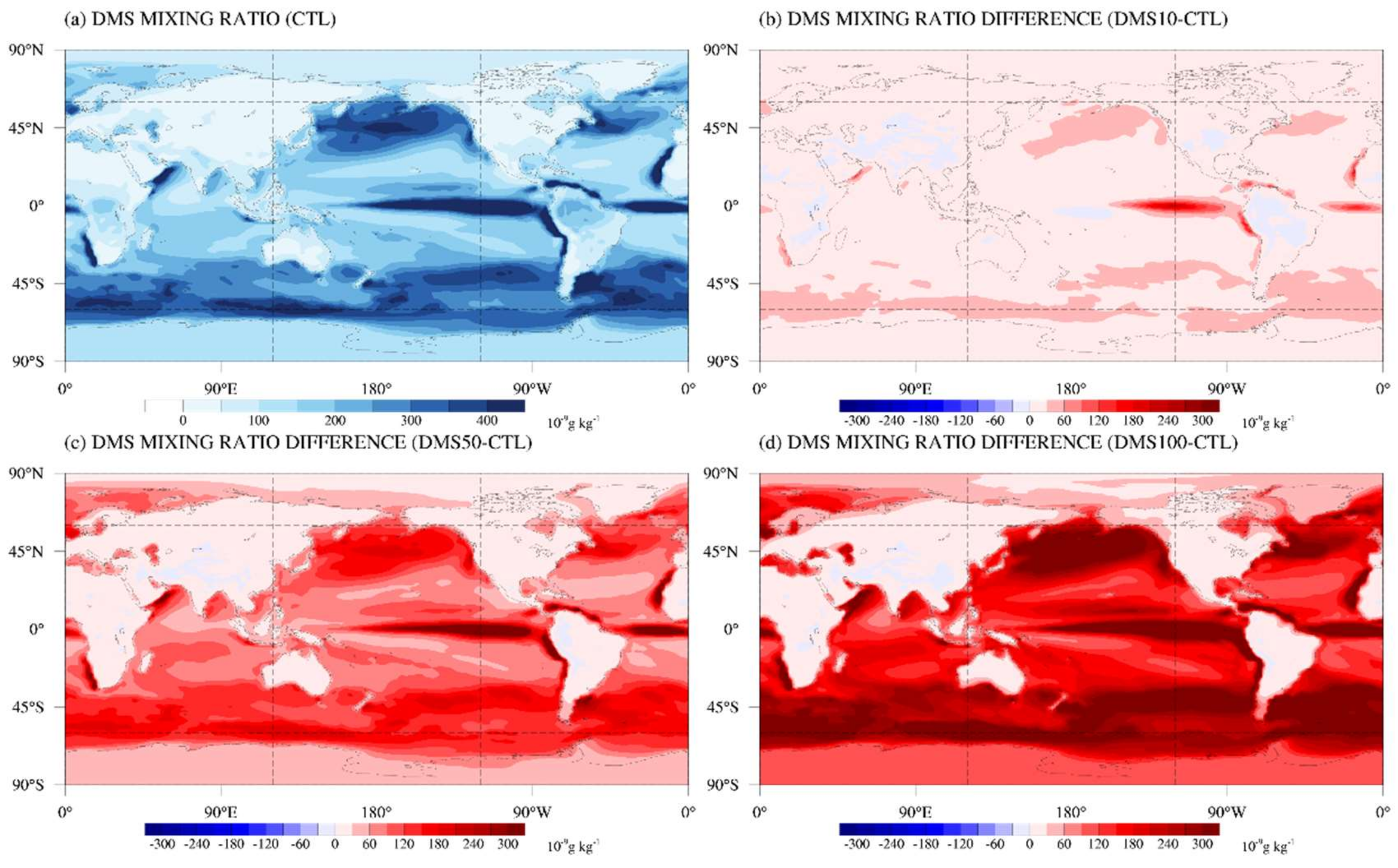
Over the oceanic regions remote from pollution sources, the major source of sulfate aerosols is DMS emitted from phytoplankton [6,35,36,37]. Figure 1a shows the mean DMS mass mixing ratio for the period from 1971 to 2000 in the CTL experiment. The DMS emission depends not only on production by phytoplankton but also on wind speed and SST [30]; thus, the DMS mixing ratio is high over the North and equatorial Pacific, the equatorial Atlantic and the Antarctic Ocean. By construction, the increase in DMS mass mixing ratio is the largest in regions with the largest mean DMS mass mixing ratio. A conspicuous increase of the DMS mixing ratio also appears in the regions where the DMS mixing ratio is high (Figure 1b–d); naturally, we can expect a corresponding increase in the sulfate aerosols in these regions.

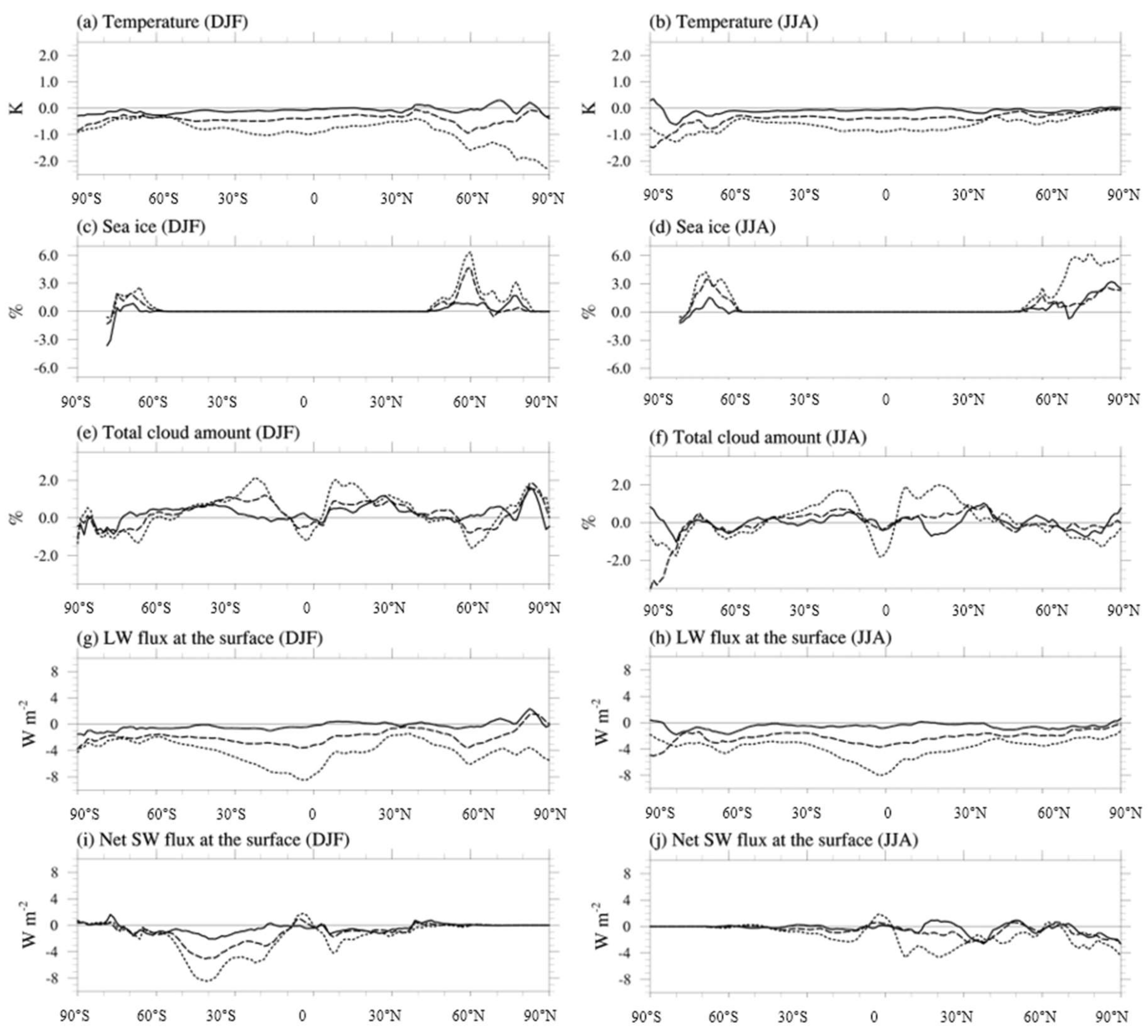
We examine how the increase of the DMS mixing ratio and thus sulfate aerosols bring about changes in relevant variables. Figure 2 shows the zonal mean difference between DMS experiments and CTL in 1.5 m temperature, sea ice fraction, cloud fraction, longwave and shortwave radiative flux at the surface for the two seasons, December, January and February (DJF) and June, July and August (JJA). Overall, the zonal mean total shortwave radiation tends to decrease mostly due to increased sulfate aerosols over the ocean directly by reflecting more sunlight and indirectly by providing more CCN and thus making the clouds brighter and longer-lasting [38,39]. The shortwave flux at the surface tends to decrease (Figure 2i), which is certainly related to the cooling effect (Figure 2a) but the cooling effect is pronounced at the latitudes where sea ice fraction increases in the winter hemisphere (Figure 2c). It turns out that the increased DMS flux resulted in the increase of sea ice fraction at the edges of the sea ice.

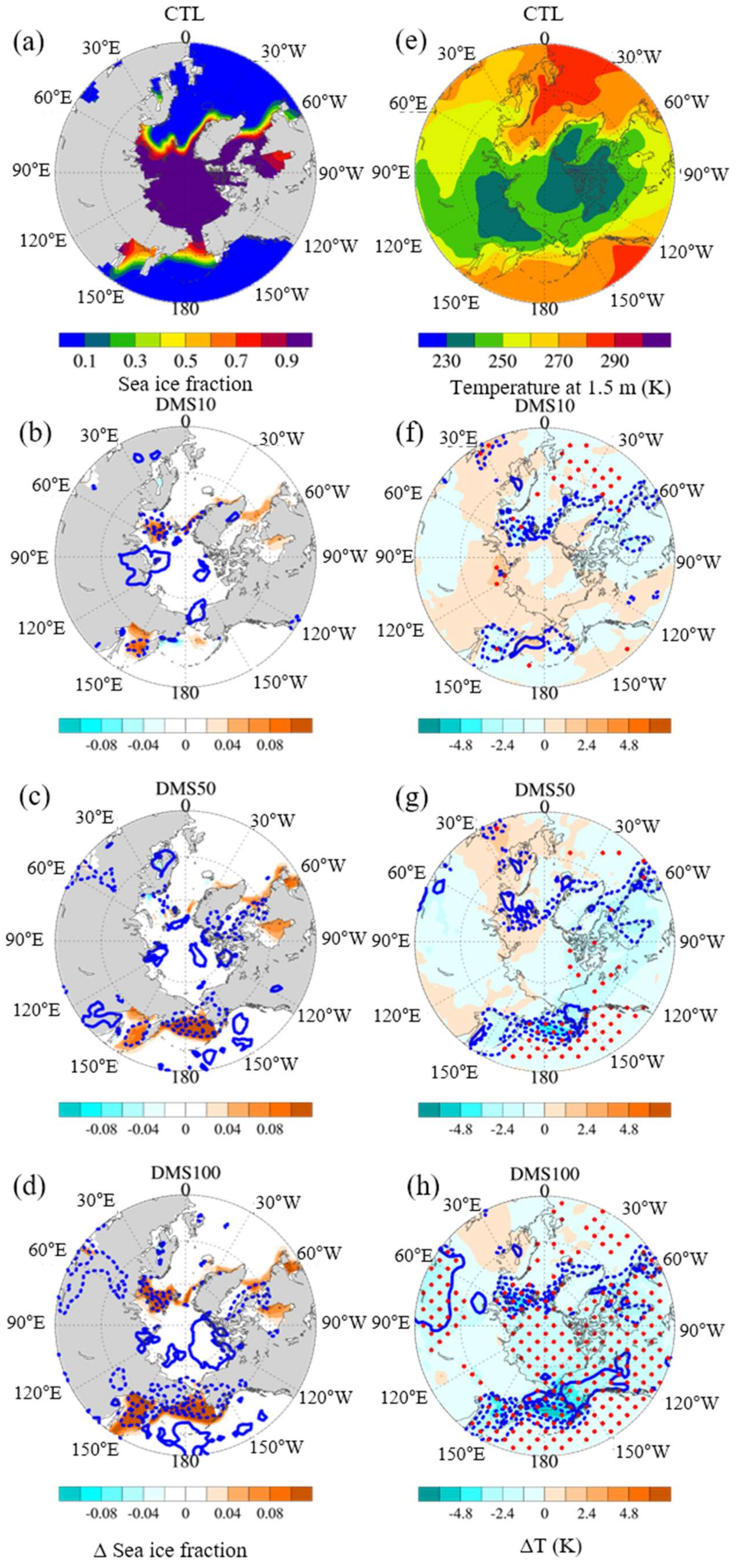
Based on the zonally averaged Arctic response, we next focus on the relationship between sea ice fraction, cloud fraction, temperature and upward longwave flux due to the change in the DMS flux over the Arctic region (higher than 45° N) in the winter season for the period of 1971–2000 (Figure 3). The Student’s t-test for the difference of mean is done for 1.5 m temperature to examine the statistical significance, following Wilks [40]. For this test, monthly mean values are used. That is, we apply the false discovery rate approach after Student’s t-test is done at all 1.5 m altitude grid points to consider the field significance. First, we rearrange the p values from smallest (p₍₁₎) to largest (p_(N)). Since the results are from the global domain, N is 27,648. For the significant level of 5% (α_global), we regard the results from the DMS experiments as being significantly different from CTL if the corresponding p values satisfy the following inequality condition:

$${\mathrm{p}}_{\left(\mathrm{j}\right)}\le \frac{\mathrm{j}}{\mathrm{N}}{\mathsf{\alpha }}_{\mathrm{global}}, \mathrm{j}=1, \dots , \mathrm{N}.$$

(2)

The regions where this inequality condition is satisfied are stippled in red in Figure 3. The results confirm that the region of statistical significance appears even for the 10% increase of DMS flux (DMS10) and that it is spread out much more widely over the globe for higher DMS flux experiments (Figure 3f–h).

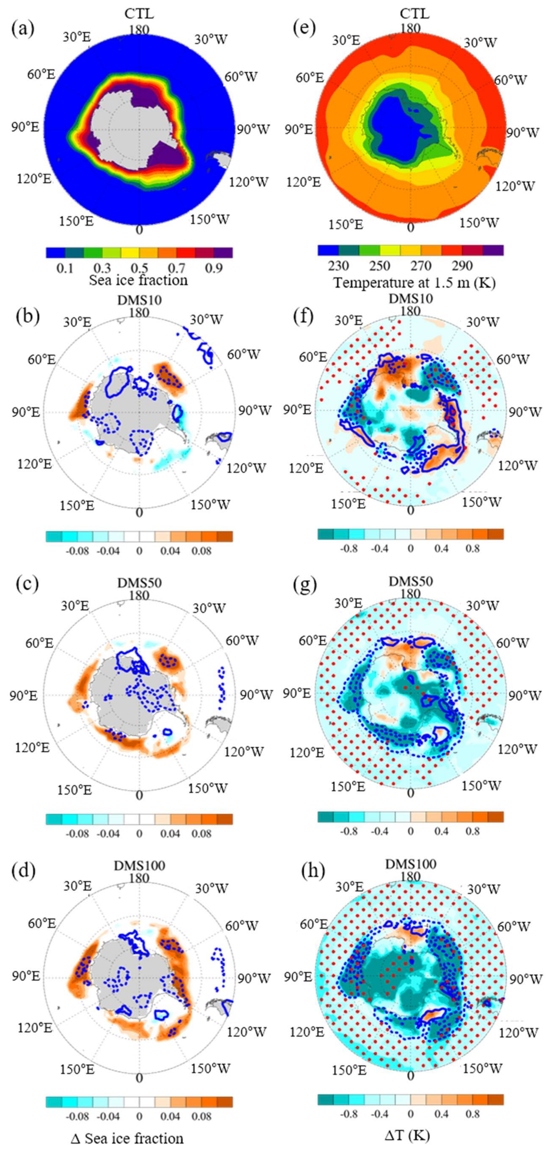
A close look at Figure 3 reveals that sea ice fraction increases at the edge areas of the sea ice with increased DMS emission experiments in winter seasons. Larger increases in the mean sea ice fraction are indicated over the Davis Strait (40° W), the Hudson Bay (80° W), the Bering Sea (180° W) and the Sea of Okhotsk (150° E) with higher DMS flux perturbations (Figure 3). These increases in sea ice fraction seem to be related to the large-scale cooling effect. An important role of sea ice is to mediate the air-sea exchange of momentum, heat, moisture and radiation [41]. Alteration of heat, moisture and radiation flux due to the increase in sea ice fraction amplifies the Arctic cooling effect. The oceanic moisture flux in the Arctic region decreases in all DMS experiments (i.e., DMS10, DMS50 and DMS100) compared to CTL by 5.43 × 10⁻⁴ g m⁻²  s⁻¹, 3.03 × 10⁻⁴ g m⁻²  s⁻¹ and 6.16 × 10⁻⁴ g m⁻² s⁻¹, respectively; this is the reason why cloud fraction decreases in these regions (for example, see the regions where sea ice fraction increases (150 E to 150 W) in Figure 3b,c,d). This is consistent with the satellite data analysis study of Boisvert et al. [42] that showed decreased moisture flux in the regions of increasing sea ice fraction. This is also where the surface upward longwave flux decreases. This indicates that the impact of heat flux blockage due to ice formation decreases the upward longwave flux. Heat flux from the ocean is blocked where sea ice is formed; therefore, surface longwave flux decreases in these regions.

Moreover, in the regions where cloud fraction decreases, the longwave cloud radiative effect (LCRE), which describes the net downward longwave flux at the top of the atmosphere under all sky conditions minus under clear sky conditions, also decreases (Figure S1). This trend extends over land regions such as Alaska. Note that the decrease of LCRE indicates an increase of upward longwave flux at the top of the atmosphere. The average values of reduced LCRE over the Arctic region in DMS10, DMS50 and DMS100 in comparison to CTL are 0.26 W m⁻², 0.35 W m⁻² and 0.53 W m⁻², respectively. In detail, larger increases in the mean sea ice fraction over in the Davis Strait (40° W), the Hudson Bay (80° W), the Bering Sea (180° W) and the Sea of Okhotsk (150° E) are indicated with higher DMS flux perturbations (Figure 3). Meanwhile, cloud fraction tends to decrease where sea ice fraction increases, which is seemingly due to the decreased moisture flux from the sea surface (Figure 3b,c,d).

Because of the polar night in the winter season, the Arctic region are unaffected by shortwave flux. Thus, surface temperature changes are associated with longwave flux changes. Longwave flux decreases significantly in the regions where sea ice fraction increases significantly. Once sea ice is formed, the heat flux from the warm sea surface is blocked by the sea ice and the longwave flux is reduced, resulting in the decrease of the surface air temperature. The regions of significant statistical differences (stippled regions) are generally similar for sea ice fraction and longwave flux. On the other hand, the pattern of temperature difference is roughly matched with that of cloud fraction, although their correspondence is weak in some regions. Clouds generally reduce the downward shortwave flux but during the period of polar night, this is not a factor. Instead, clouds act as a blanket; thus, a decrease in cloud fraction reduces the LCRE in this case.

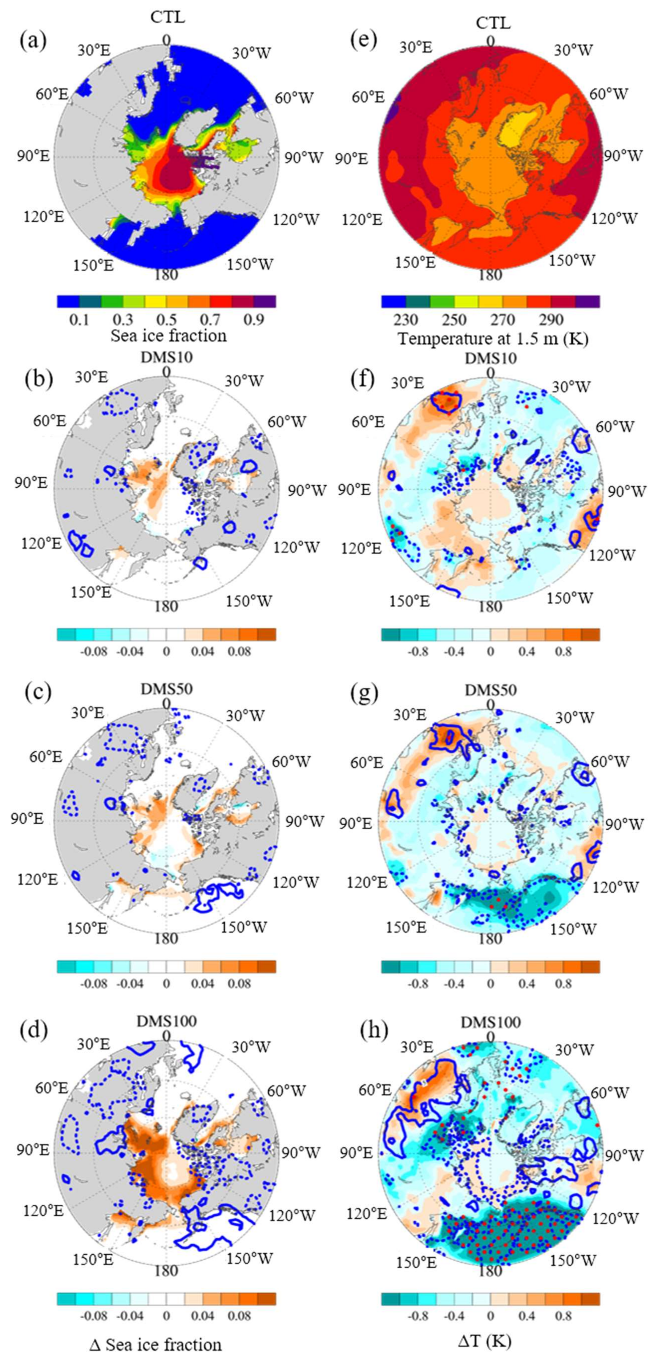
In the summer season (Figure 4), sea ice fraction increases with the DMS increase over the Arctic Sea regions where sea ice melts during the summer in CTL (Figure 4b,c,d). The relationships between temperature and other variables appear to be different from those in winter. Temperature changes are generally small compared to those in the winter season. For DMS10 (Figure 4b,f), the temperature difference is generally negatively associated with the cloud fraction difference but positively correlated with the shortwave flux difference. Increase in cloud fraction reduces the downward shortwave flux and therefore the opposite trend of the cloud fraction difference and the shortwave flux difference in Figure 4 is understandable. To quantitatively assess this relationship, the difference of the cloud fraction between the DMS experiments and CTL and that of the shortwave cloud radiative effect (SCRE), which describes the net downward shortwave radiation under all sky conditions minus under clear sky conditions at the top of the atmosphere, are obtained at individual grid points and the correlation coefficient of the linear regression between the two difference values are calculated. They are −0.70, −0.75 and −0.78 for DMS10-CTL, DMS50-CTL and DMS100-CTL, respectively, convincingly demonstrating the negative relationship between cloud fraction and the net downward shortwave flux.

The reduced downward shortwave flux then leads to a decrease of surface temperature. Consistently, in DMS50 and DMS100, the temperature decrease is pronounced where additional sea ice is formed (150 E to 120 W) (Figure 4g,h). In polar regions, global temperature reduction leads to increase in sea ice thickness and fraction and thereby enhancing surface albedo that causes the ice-albedo feedback mechanism [41]. The enhanced surface albedo amplifies the polar cooling effect by reflecting more sunlight. Demonstrated in Figure S2 are such negative correlations between temperature changes versus ice albedo changes in DMS simulations in comparison to CTL at individual grid points. The reduced downward shortwave flux then leads to a decrease in the surface temperature.

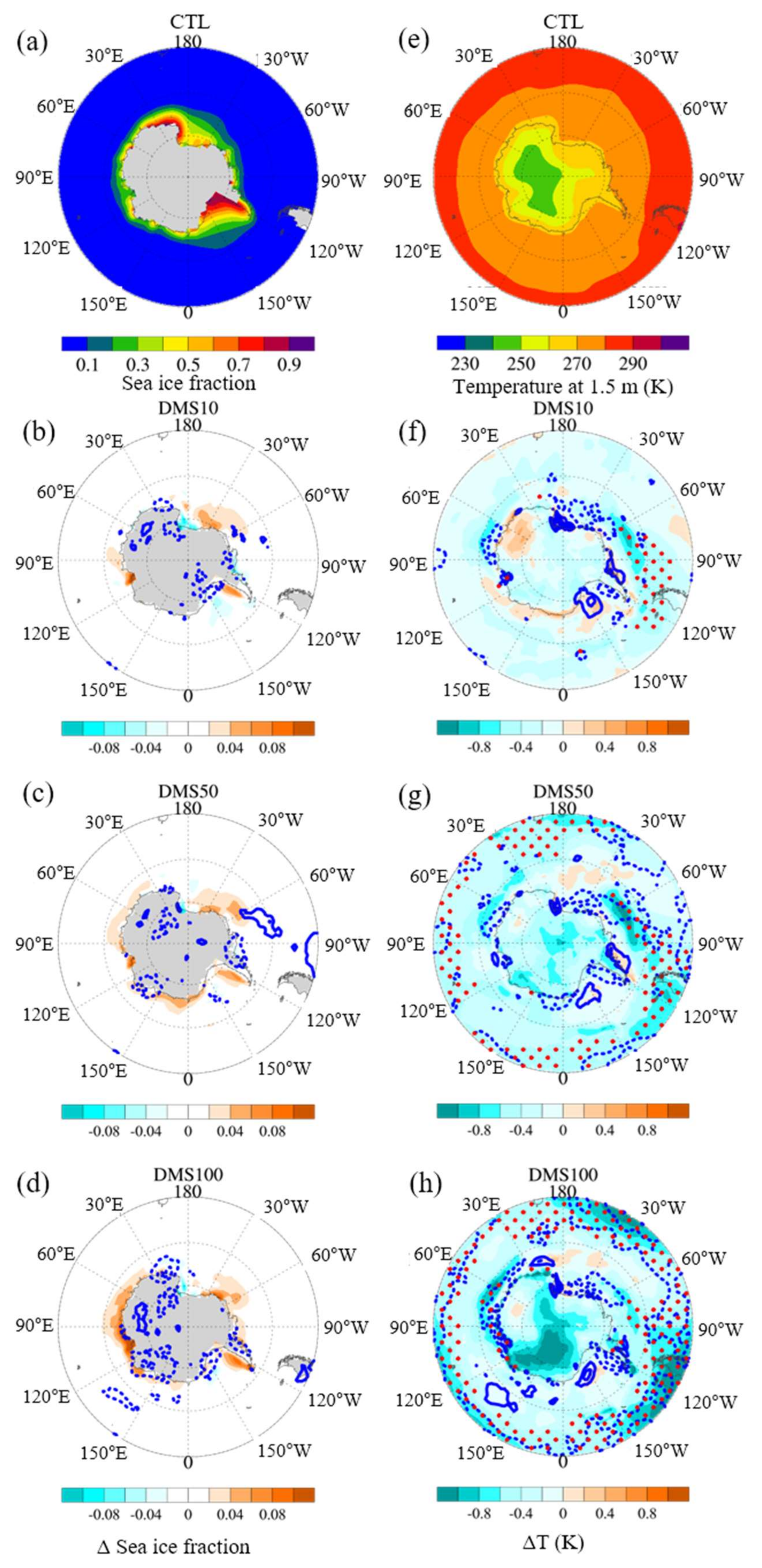
The Antarctic region show the results that are mostly consistent with those of the Arctic region as shown in Figure 5 for winter season (JJA). The temperature changes significantly over the oceans with increase DMS flux. Changes in sea ice fraction are larger at the higher DMS perturbation experiments: for example, see the Amundsen Sea (150° W) region. Decrease in upward longwave flux over the places where sea ice fraction increases are also shown in the Antarctic region. The oceanic moisture fluxes in the Antarctic region decrease by 5.41 × 10⁻⁴ g m⁻² s⁻¹, 5.03 × 10⁻⁴ g m⁻² s⁻¹ and 5.56 × 10⁻⁴ g m⁻² s⁻¹ for DMS10, DMS50 and DMS100, respectively, when compared to CTL. Decrease of cloud fraction is pronounced where sea ice fraction is decreased as shown in Figure 5b–d. However, such changes are not exactly temporally matched because there is a time lag in their changes [43]. Decreases in moisture flux, in turn, reduce LCRE by 0.08 W m⁻², 0.27 W m⁻² and 0.62 W m⁻², for DMS10, DMS50 and DMS100, respectively, when compared to CTL. Such reduction of incoming radiative energy leads to general decrease of the temperature over the oceans (Figure 5f–h).

Compared to the winter season increase of sea ice fraction in the DMS experiments is smaller in the summer season in the Antarctic region (Figure 6). However, reduction of the net downward shortwave flux over the regions of increased sea ice fraction and the general trend of decreasing 1.5 m temperature is still maintained (Figure 6f–h). Overall such features of the DMS experiments are similar to those of the Arctic region.

4. Discussion and Conclusions

This study examines the impact of increased oceanic DMS fluxes on climate especially in polar regions using the HadGEM2-AO, a coupled atmosphere-ocean model. Increased DMS imposes more sulfate aerosols over oceanic atmosphere. Locally increased oceanic sulfate aerosols contribute to higher CCN concentration and larger cloud fraction over the oceans. Such cloud fraction change results in the net cooling effects over the oceans and consequently cool the Earth surface. The Polar regions (i.e., the Arctic and Antarctic regions) are the most susceptible to climate changes and thereby expanding sea ice. In winter season, the enlarged sea ice fraction impedes the air-sea exchange of moisture and heat fluxes. Low level air temperature decreases locally where the ocean heat flux is blocked. Decreased moisture flux reduces cloud locally and the local air temperature decreases further with reduced LCRE. In summer season, the increased sea ice fraction induces positive ice-albedo feedback and hence decreases temperature.

The important result obtained in this study is that increase in DMS emissions, supposedly due to increase of phytoplankton biomass under global warming conditions, can lead to increase in sulfate aerosols and eventually contribute to polar cooling effect by increasing sea ice fraction. This is different from Park et al. [20], who only emphasized the effect of changes in shortwave absorption due to increased phytoplankton from biophysical feedback. In particular, the polar regions are highly sensitive to ice albedo feedback, temperature lapse rate feedback and water vapor/cloud feedback [20,44,45]. Consistently, this study shows that in the polar regions, temperature responses can be amplified by changes in sea ice fraction, even for DMS10, which prescribes only a 10% increase in the DMS emission flux.

Global warming can change the activity of phytoplankton biomass. As noted, several previous studies suggested that increased phytoplankton biomass could enhance global warming and amplify the Arctic warming by increasing the SST and sea ice melting [9,10,20,46]. However, other studies found a negative feedback by ocean DMS production [26,47]. In this study, we also demonstrate that the increase in phytoplankton and consequent increase in DMS emissions can induce large-scale cooling effect. The cooling effect is concentrated in the polar regions due to the increase of sea ice fraction. However, the cooling effect can, in turn, reduce DMS emissions due to decrease in phytoplankton physiological activity, which may again lead to local warming in the polar regions. Boyce et al. [48] showed that observed long-term global phytoplankton concentrations have declined over the past century, especially in tropical and subtropical oceans where increased SST might have strengthened ocean stratification and therefore reduced the nutrient supply from the water below. On the other hand, updated climatological data from ship observations [49] have indicated that the DMS flux was 17% stronger than that reported by Kettle et al. [29], which was used as the climatological data in this study. This means that the current understanding of DMS emission changes under global warming condition is still highly uncertain.

Furthermore, according to Carslaw et al. [50], the uncertainty range of aerosol indirect radiative forcing from the DMS flux perturbation was one of the largest among the 28 parameters that were related to aerosol indirect radiative forcing, including natural and anthropogenic aerosol emissions. In this study, we did not perform reduced DMS emission experiments but our results of enhanced cooling effect due to increased DMS emissions could also imply, if the response is linear, that the global reduction of phytoplankton and therefore reduced DMS emissions could increase the surface temperature and reduce sea ice fraction in the polar regions. That is, global warming can also be amplified due to the reduction of phytoplankton and thus DMS emissions. Six et al. [14] pointed out that current seawater pH values are reduced compared to those in preindustrial times and demonstrated that the reduced DMS emissions resulting from such ocean acidification could amplify global warming.

Feedback by DMS and phytoplankton cannot be simply estimated. An obvious result of this modeling study is that perturbations in DMS emission could cause significant climate change, especially in the polar regions. However, the current climate models do not comprehensively incorporate these opposite effects of DMS and phytoplankton. Only when these opposite effects are properly considered in future climate models, it may be possible to estimate which effect is more important and the implications of this result would be meaningful in future climate predictions.

References

- Gondwe, M.; Krol, M.; Gieskes, W.; Klaassen, W.; de Baar, H. The contribution of ocean-leaving DMS to the global atmospheric burdens of DMS, MSA, SO2, and NSS . Global Biogeochem. Cycles 2003, 17. [Google Scholar] [CrossRef]
- Kloster, S.; Feichter, J.; Maier-Reimer, E.; Six, K.D.; Stier, P.; Wetzel, P. DMS cycle in the marine ocean-atmosphere system-A global model study. Biogeosciences 2006, 3, 29–51. [Google Scholar] [CrossRef]
- Bopp, L.; Monfray, P.; Aumont, O.; Dufesne, J.L.; Le Treut, H.; Madec, G.; Terray, L.; Orr, J.C. Potential impact of climate change on marine export production. Global Biogeochem. Cycles 2001, 15, 81–99. [Google Scholar] [CrossRef] [Green Version]
- Gabric, A.J.; Simo, R.; Cropp, R.A.; Hirst, A.; Dachs, J. Modeling estimates of the global emission of dimethylsulfide under enhanced greenhouse conditions. Global Biogeochem. Cycles 2004, 18. [Google Scholar] [CrossRef] [Green Version]
- IPCC. Climate Change 2013: The Physical Science Basis. Contribution of Working Group i to the Fifth Assessment Report of the Intergovernmental Panel on Climate Change; Cambridge University Press: Cambridge, UK; New York, NY, USA, 2013; p. 1535. [Google Scholar]
- Charlson, R.J.; Lovelock, J.E.; Andreae, M.O.; Warren, S.G. Oceanic phytoplankton, atmospheric sulphur, cloud albedo and climate. Nature 1987, 326, 655. [Google Scholar] [CrossRef]
- Ayers, G.P.; Cainey, J.M. The claw hypothesis: A review of the major developments. Environ. Chem. 2007, 4, 366–374. [Google Scholar] [CrossRef]
- Lovelock, J. The Revenge of Gaia: Earth’s Climate Crisis & the Fate of Humanity; Basic Books: New York, NY, USA, 2006. [Google Scholar]
- Frouin, R.; Iacobellis, S. Influence of phytoplankton on the global radiation budget. J. Geophys. Res. Atmos. 2002, 107, ACL–5. [Google Scholar] [CrossRef]
- Patara, L.; Vichi, M.; Masina, S.; Fogli, P.G.; Manzini, E. Global response to solar radiation absorbed by phytoplankton in a coupled climate model. Clim. Dyn. 2012, 39, 1951–1968. [Google Scholar] [CrossRef]
- Henson, S.A.; Sarmiento, J.L.; Dunne, J.P.; Bopp, L.; Lima, I.; Doney, S.C.; John, J.; Beaulieu, C. Detection of anthropogenic climate change in satellite records of ocean chlorophyll and productivity. Biogeosciences 2010, 7, 621–640. [Google Scholar] [CrossRef] [Green Version]
- Jochum, M.; Yeager, S.; Lindsay, K.; Moore, K.; Murtugudde, R. Quantification of the feedback between phytoplankton and ENSO in the community climate system model. J. Clim. 2010, 23, 2916–2925. [Google Scholar] [CrossRef]
- Kloster, S.; Six, K.D.; Feichter, J.; Maier-Reimer, E.; Roeckner, E.; Wetzel, P.; Stier, P.; Esch, M. Response of dimethylsulfide (DMS) in the ocean and atmosphere to global warming. J. Geophys. Res. 2007, 112, G03005. [Google Scholar] [CrossRef]
- Six, K.D.; Kloster, S.; Ilyina, T.; Archer, S.D.; Zhang, K.; Maier-Reimer, E. Global warming amplified by reduced sulphur fluxes as a result of ocean acidification. Nat. Clim. Chang. 2013, 3, 975. [Google Scholar] [CrossRef]
- Timmermann, A.; Jin, F.F. Phytoplankton influences on tropical climate. Geophys. Res. Lett. 2002, 29, 19-1–19-4. [Google Scholar] [CrossRef]
- Korhonen, H.; Carslaw, K.S.; Spracklen, D.V.; Mann, G.W.; Woodhouse, M.T. Influence of oceanic dimethyl sulfide emissions on cloud condensation nuclei concentrations and seasonality over the remote southern hemisphere oceans: A global model study. J. Geophys. Res. Atmos. 2008, 113. [Google Scholar] [CrossRef]
- Thomas, M.A.; Suntharalingam, P.; Pozzoli, L.; Devasthale, A.; Kloster, S.; Rast, S.; Feichter, J.; Lenton, T.M. Rate of non-linearity in DMS aerosol-cloud-climate interactions. Atmos. Chem. Phys. 2011, 11, 11175–11183. [Google Scholar] [CrossRef] [Green Version]
- Thomas, M.A.; Suntharalingam, P.; Pozzoli, L.; Rast, S.; Devasthale, A.; Kloster, S.; Feichter, J.; Lenton, T.M. Quantification of DMS aerosol-cloud-climate interactions using the echam5-hammoz model in a current climate scenario. Atmos. Chem. Phys. 2010, 10, 7425–7438. [Google Scholar] [CrossRef] [Green Version]
- Wingenter, O.W.; Elliot, S.M.; Blake, D.R. New directions: Enhancing the natural sulfur cycle to slow global warming. Atmos. Environ. 2007, 41, 7373–7375. [Google Scholar] [CrossRef]
- Park, J.-Y.; Kug, J.-S.; Bader, J.; Rolph, R.; Kwon, M. Amplified arctic warming by phytoplankton under greenhouse warming. Proc. Nat. Acad. Sci. USA 2015, 112, 5921–5926. [Google Scholar] [CrossRef] [PubMed]
- Arrigo, K.R.; Van Dijken, G.; Pabi, S. Impact of a shrinking arctic ice cover on marine primary production. Geophys. Res. Lett. 2008, 35. [Google Scholar] [CrossRef]
- Arrigo, K.R.; Perovich, D.K.; Pickart, R.S.; Brown, Z.W.; van Dijken, G.L.; Lowry, K.E.; Mills, M.M.; Palmer, M.A.; Balch, W.M.; Bahr, F.; et al. Massive phytoplankton blooms under arctic sea ice. Science 2012, 336, 1408. [Google Scholar] [CrossRef] [PubMed]
- Popova, E.E.; Yool, A.; Coward, A.C.; Dupont, F.; Deal, C.; Elliott, S.; Hunke, E.; Jin, M.; Steele, M.; Zhang, J. What controls primary production in the arctic ocean? Results from an intercomparison of five general circulation models with biogeochemistry. J. Geophys. Res. 2012, 117. [Google Scholar] [CrossRef]
- Stroeve, J.C.; Kattsov, V.; Barrett, A.; Serreze, M.; Pavlova, T.; Holland, M.; Meier, W.N. Trends in arctic sea ice extent from CMIP5, CMIP3 and observations. Geophys. Res. Lett. 2012, 39. [Google Scholar] [CrossRef]
- Vancoppenolle, M.; Bopp, L.; Madec, G.; Dunne, J.; Ilyina, T.; Halloran, P.R.; Steiner, N. Future arctic ocean primary productivity from CMIP5 simulations: Uncertain outcome, but consistent mechanisms. Glob. Biogeochem. Cycles 2013, 27, 605–619. [Google Scholar] [CrossRef] [Green Version]
- Gunson, J.; Spall, S.; Anderson, T.; Jones, A.; Totterdell, I.; Woodage, M. Climate sensitivity to ocean dimethylsulphide emissions. Geophys. Res. Lett. 2006, 33. [Google Scholar] [CrossRef] [Green Version]
- Martin, G.M.; Milton, S.F.; Senior, C.A.; Brooks, M.E.; Ineson, S.; Reichler, T.; Kim, J. Analysis and reduction of systematic errors through a seamless approach to modeling weather and climate. J. Clim. 2010, 23, 5933–5957. [Google Scholar] [CrossRef]
- Halloran, P.R.; Bell, T.G.; Totterdell, I.J. Can we trust empirical marine DMS parameterisations within projections of future climate? Biogeosciences 2010, 7, 1645–1656. [Google Scholar] [CrossRef] [Green Version]
- Kettle, A.J.; Andreae, M.O. Flux of dimethylsulfide from the oceans: A comparison of updated data sets and flux models. J. Geophys. Res. Atmos. 2000, 105, 26793–26808. [Google Scholar] [CrossRef] [Green Version]
- Jones, A.; Roberts, D.L. An Interactive DMS Emissions Scheme for the Unified Model; Met Office: Exeter, UK, 2004. [Google Scholar]
- Saltzman, E.; King, D.; Holmen, K.; Leck, C. Experimental determination of the diffusion coefficient of dimethylsulfide in water. J. Geophys. Res. Oceans 1993, 98, 16481–16486. [Google Scholar] [CrossRef]
- Collins, W.J.; Bellouin, N.; Doutriaux-Boucher, M.; Gedney, N.; Halloran, P.; Hinton, T.; Hughes, J.; Jones, C.D.; Joshi, M.; Liddicoat, S. Development and evaluation of an earth-system model-HadGEM2. Geosci. Model Dev. 2011, 4, 1051–1075. [Google Scholar] [CrossRef]
- Jones, A.; Haywood, J.M. Sea-spray geoengineering in the hadgem2-es earth-system model: Radiative impact and climate response. Atmos. Chem. Phys. 2012, 12, 10887–10898. [Google Scholar] [CrossRef] [Green Version]
- Taylor, K.E.; Stouffer, R.J.; Meehl, G.A. An overview of CMIP5 and the experiment design. Bull. Am. Meteorol. Soc. 2012, 93, 485–498. [Google Scholar] [CrossRef]
- Andreae, M.O.; Crutzen, P.J. Atmospheric aerosols: Biogeochemical sources and role in atmospheric chemistry. Science 1997, 276, 1052–1058. [Google Scholar] [CrossRef]
- Hoffmann, E.H.; Tilgner, A.; Schrodner, R.; Brauer, P.; Wolke, R.; Herrmann, H. An advanced modeling study on the impacts and atmospheric implications of multiphase dimethyl sulfide chemistry. Proc. Natl. Acad. Sci. USA 2016, 113, 11776–11781. [Google Scholar] [CrossRef] [PubMed] [Green Version]
- Hopkins, F.E.; Archer, S.D. Consistent increase in dimethyl sulfide (DMS) in response to high CO2 in five shipboard bioassays from contrasting NW European waters. Biogeosciences 2014, 11, 4925–4940. [Google Scholar] [CrossRef]
- Albrecht, B.A. Aerosols, cloud microphysics, and fractional cloudiness. Science 1989, 245, 1227–1230. [Google Scholar] [CrossRef] [PubMed]
- Twomey, S. The influence of pollution on the shortwave albedo of clouds. J. Atmos. Sci. 1977, 34, 1149–1152. [Google Scholar] [CrossRef]
- Wilks, D.S. The stippling shows statistically significant grid points: How research results are routinely overstated and overinterpreted, and what to do about it. Bull. Am. Meteorol. Soc. 2016, 97, 2263–2273. [Google Scholar] [CrossRef]
- Curry, J.A.; Schramm, J.L.; Ebert, E.E. Sea ice-albedo climate feedback mechanism. J.Clim. 1995, 8, 240–247. [Google Scholar] [CrossRef]
- Boisvert, L.N.; Markus, T.; Vihma, T. Moisture flux changes and trends for the entire arctic in 2003–2011 derived from EOS aqua data. J. Geophys. Res. Oceans 2013, 118, 5829–5843. [Google Scholar] [CrossRef]
- Abe, M.; Nozawa, T.; Ogura, T.; Takata, K. Effect of retreating sea ice on arctic cloud cover in simulated recent global warming. Atmos. Chem. Phys. 2016, 16, 14343–14356. [Google Scholar] [CrossRef]
- Graversen, R.G.; Wang, M. Polar amplification in a coupled climate model with locked albedo. Clim. Dyn. 2009, 33, 629–643. [Google Scholar] [CrossRef]
- Winton, M. Amplified arctic climate change: What does surface albedo feedback have to do with it? Geophys. Res. Lett. 2006, 33. [Google Scholar] [CrossRef]
- Manizza, M.; Le Quërë, C.; Watson, A.J.; Buitenhuis, E.T. Bio-optical feedbacks among phytoplankton, upper ocean physics and sea-ice in a global model. Geophys. Res. Lett. 2005, 32. [Google Scholar] [CrossRef]
- Bopp, L.; Boucher, O.; Aumont, O.; Belviso, S.; Dufresne, J.-L.; Pham, M.; Monfray, P. Will marine dimethylsulfide emissions amplify or alleviate global warming? A model study. Can. J. Fish. Aquat. Sci. 2004, 61, 826–835. [Google Scholar] [CrossRef]
- Boyce, D.G.; Lewis, M.R.; Worm, B. Global phytoplankton decline over the past century. Nature 2010, 466, 591. [Google Scholar] [CrossRef] [PubMed]
- Lana, A.; Bell, T.G.; Simó, R.; Vallina, S.M.; Ballabrera-Poy, J.; Kettle, A.J.; Dachs, J.; Bopp, L.; Saltzman, E.S.; Stefels, J. An updated climatology of surface dimethlysulfide concentrations and emission fluxes in the global ocean. Global Biogeochem. Cycles 2011, 25. [Google Scholar] [CrossRef] [Green Version]
- Carslaw, K.S.; Lee, L.A.; Reddington, C.L.; Pringle, K.J.; Rap, A.; Forster, P.M.; Mann, G.W.; Spracklen, D.V.; Woodhouse, M.T.; Regayre, L.A. Large contribution of natural aerosols to uncertainty in indirect forcing. Nature 2013, 503, 67. [Google Scholar] [CrossRef] [PubMed]
Figure 1.
Mean dimethyl-sulfide mass mixing ratio for the period 1971–2000 from control run (CTL) (a) and its differences between DMS10 and CTL (b), DMS50 and CTL (c) and DMS100 and CTL (d).
Figure 2.
Zonal and annual mean differences of temperature at 1.5 m altitude (a,b), sea ice fraction (c,d), cloud fraction (e,f), upward longwave flux at the surface (g,h) and net shortwave flux at the surface (i,j) between DMS10 and CTL (solid line), DMS50 and CTL (dashed line) and DMS100 and CTL (dotted line) experiments for December, January and February (DJF) (left panels) and for June, July and August (JJA) (right panels) for the period 1971–2000.
Figure 3.
Upper panels: sea ice fraction (a) and the differences of sea ice fraction (shading, %) and cloud fraction (solid and dashed lines for positive and negative values, respectively, every 2.5%) between DMS10 and CTL (b), DMS50 and CTL (c) and DMS 100 and CTL (d) experiments. Lower panels: temperature at 1.5 m altitude (e) and the differences of temperature (shading, K) and upward longwave flux at the surface (solid lines indicate the values of 4, 24 and 44 W m−2 and dashed lines indicate the values of −4, −24 and −44 W m−2) between DMS10 and CTL (f), DMS50 and CTL (g) and DMS 100 and CTL (h) experiments. These results are for DJF during 1971–2000 in the Arctic region (45° N–90° N). Red stipples indicate the regions where the null hypothesis of “no difference of seasonal average temperature at 1.5 m altitude between CTL and increased DMS experiments” is rejected at 5% test level.
Figure 4.
Upper panels: sea ice fraction (a) and the differences of sea ice fraction (shading, %) and cloud fraction (solid and dashed lines for positive and negative values, respectively, every 2.5%) between DMS10 and CTL (b), DMS50 and CTL (c) and DMS 100 and CTL (d) experiments. Lower panels: temperature at 1.5 m altitude (e) and the differences of temperature (shading, K) and downward shortwave flux at the surface (solid and dashed lines indicate positive and negative values, respectively, every 5 W m−2). These results are for JJA during 1971–2000 in the Arctic region (45°N–90°N). Red stipples indicate the regions where the null hypothesis of “no difference of seasonal average temperature at 1.5 m altitude between CTL and increased DMS experiments” is rejected at 5% test level.
Figure 5.
Upper panels: sea ice fraction (a) and the differences of sea ice fraction (shading, %) and cloud fraction (solid and dashed lines for positive and negative values, respectively, every 2.5%) between DMS10 and CTL (b), DMS50 and CTL (c) and DMS 100 and CTL (d) experiments. Lower panels: temperature at 1.5 m altitude (e) and the differences of temperature (shading, K) and upward longwave flux at the surface (solid lines indicate the values of 4, 24 and 44 W m−2 and dashed lines indicate the values of −4, −24 and −44 W m−2) between DMS10 and CTL (f), DMS50 and CTL (g) and DMS 100 and CTL (h) experiments. These results are for JJA during 1971–2000 in the Antarctic region (45° S–90° S). Red stipples indicate the regions where the null hypothesis of “no difference of seasonal average temperature at 1.5 m altitude between CTL and increased DMS experiments” is rejected at 5% test level.
Figure 6.
Upper panels: sea ice fraction (a) and the differences of sea ice fraction (shading, %) and cloud fraction (solid and dashed lines for positive and negative values, respectively, every 2.5%) between DMS10 and CTL (b), DMS50 and CTL (c) and DMS 100 and CTL (d) experiments. Lower panels: temperature at 1.5 m altitude (e) and the differences of temperature (shading, K) and downward shortwave flux at the surface (solid and dashed lines indicate positive and negative values, respectively, every 5 W m−2). These results are for DJF during 1971–2000 in the Antarctic region (45° S–90° S). Red stipples indicate the regions where the null hypothesis of “no difference of seasonal average temperature at 1.5 m altitude between CTL and increased DMS experiments” is rejected at 5% test level.
© 2018 by the authors. Licensee MDPI, Basel, Switzerland. This article is an open access article distributed under the terms and conditions of the Creative Commons Attribution (CC BY) license (http://creativecommons.org/licenses/by/4.0/).
Share and Cite
MDPI and ACS Style
Kim, A.-H.; Yum, S.S.; Lee, H.; Chang, D.Y.; Shim, S. Polar Cooling Effect Due to Increase of Phytoplankton and Dimethyl-Sulfide Emission. Atmosphere 2018, 9, 384. https://doi.org/10.3390/atmos9100384
AMA Style
Kim A-H, Yum SS, Lee H, Chang DY, Shim S. Polar Cooling Effect Due to Increase of Phytoplankton and Dimethyl-Sulfide Emission. Atmosphere. 2018; 9(10):384. https://doi.org/10.3390/atmos9100384
Chicago/Turabian StyleKim, Ah-Hyun, Seong Soo Yum, Hannah Lee, Dong Yeong Chang, and Sungbo Shim. 2018. "Polar Cooling Effect Due to Increase of Phytoplankton and Dimethyl-Sulfide Emission" Atmosphere 9, no. 10: 384. https://doi.org/10.3390/atmos9100384
Note that from the first issue of 2016, this journal uses article numbers instead of page numbers. See further details here.