Local Convection and Turbulence in the Amazonia Using Large Eddy Simulation Model


1
National Institute for Space Researcb (INPE), São José dos Campos 12227-010, State of São Paulo, Brazil
2
Centro Tecnico Aeroespacial (CTA/IAE), São José dos Campos 12228904, State of São Paulo, Brazil
3
Institute of Meteorology and Climatology, Leibniz University Hannover, 30167 Hannover, Germany
*
Authors to whom correspondence should be addressed.
†
Current Address: Engineering and Geosciences Institute, Federal University ofWest of Para (UFOPA), Santarém 68040-255, State of Pará, Brazil.
Atmosphere 2018, 9(10), 399; https://doi.org/10.3390/atmos9100399
Submission received: 27 June 2018
/
Revised: 11 September 2018
/
Accepted: 13 September 2018
/
Published: 12 October 2018
(This article belongs to the Special Issue Large-Eddy Simulations (LES) of Atmospheric Boundary Layer Flows)
Abstract
:Using a high resolution model of Large Eddies Simulation (LES), named PALM from PArallel LES Model, a set of simulations were performed to understand how turbulence and convection behave in a pasture and forest sites in Amazonia during the dry and rainy seasons. Related to seasonality, dry period presented higher differences of values (40 W m−2) and patterns over the sites, while in the wet period have more similar characteristics (difference of −10 W m−2). The pasture site had more convection than the forest, with effective mixing and a deeper boundary layer (2600 m). The vertical decrease of sensible heat flux with altitude fed convection and also influenced the convective boundary layer (CBL) height. Regarding the components of turbulent kinetic energy equation, the thermal production was the most important component and the dissipation rate responded with higher growth, especially in cases of greatest mechanical production at the forest surface reaching values up to −20.0.
1. Introduction
The Amazon region is the largest rainforest on the planet and it is currently a large focus of scientific research because of its influence on climate. As an example, there are several experiments taking place led by LBA (Large Scale Biosphere—Atmosphere Experiment in Amazonia) together with several countries, where amongst the various objectives is to understand better the interactions between forest and atmosphere Recently, new experiments, such as the ATTO (Amazon Tall Tower Observatory [1]), GoAmazon2014/15 (Green Ocean Amazon [2]) and ACRIDICON [3] have been installed.
Although the Amazon basin has great climatic significance, systematic errors in weather forecasts [4] and climate analyzes are still observed due to lack of complete understanding of Amazonian atmospheric characteristics, especially regarding the replacement of forests by pasture sites. It is known that the Amazon forest preserves by recycling moist air passing over it, which brings rainfall to inner areas, distant from the oceans, in the continent. This is achieved by the innate ability of trees to transfer large volumes of soil water into the atmosphere through evapotranspiration. Contributing to local [5], regional [6,7] and global [8,9] processes. From 1980 to 2007, Amazon deforestation reached 432,000 square kilometers, which corresponds to almost 15% of the Amazon region, a figure that is still growing. This substitution leads to changes in climatic conditions [10,11], which need to be studied to know the complete impact of these changes, especially with respect to the Planetary Boundary Layer (PBL).
A previous study [12] observed that the main cause of precipitation in the macro- and meso-scale circulation in the Amazon region and the dynamic processes can be grouped into three types: (a) daytime convection resulting from surface heating and favorable large-scale conditions; (b) instability lines originated in the north-northeast coast of the Atlantic; and (c) convective Cumulonimbus clusters of meso- and large-scale associated with the penetration of frontal systems in the S/SE region of Brazil and interacting with the Amazon region. Thus, it can be noted that this region is strongly influenced by convection, having the most intense convective precipitation of South America [13], determining the convection heating as an important mechanism of the tropical atmosphere and its variants in terms of intensity and position. According to Horel et al. [14], the positions of strong convective activity and consequent rainfall is related to seasonality, in which the northwest (southeast) of the Amazon Basin monthly rainfall develops during the Southern winter (summer).
The current advances in computer sciences and other analysis tools are used to do general modeling studies, particularly in the micrometeorology area. While these advances for large scale numerical simulation allow the insertion of new and more comprehensive data and equations for an improvement in model results, modeling at other scales, such as the use of Large-Eddy Simulations (LES), allows for combinations of processes with a good reduction of the computational cost and providing deeper analysis of smaller scale phenomena. Examples of common use of turbulence-resolving LES in microscale studies is the interaction between the surface and the convective boundary layer (CBL) by resolving the bulk of the energy-containing eddies that has been exploited by several different groups [15,16,17,18,19]. The LES model is a very powerful tool, and its use increases the knowledge of the convective boundary layer characteristics that are not commonly measured, such as turbulent kinetic energy balance, entrainment fluxes at the top of CBL and the temporal variation of the CBL growth, amongst others.
The main objective of this work was to conduct analyses of the behavior of heat and humidity flows in the convective boundary layer associated with surface conditions by using a high resolution LES numerical mode to better understand the patterns of turbulence and convection in different Amazonian sites. For this, cells and convective structure characteristics and their occurrence were analyzed on two different contrasting surface types, a site which is covered by pasture (a deforested area) and the other by a primary forest region for different seasons (dry and wet periods).
2. LES Model and Simulation Set-Up
2.1. Sites and Data Experiments
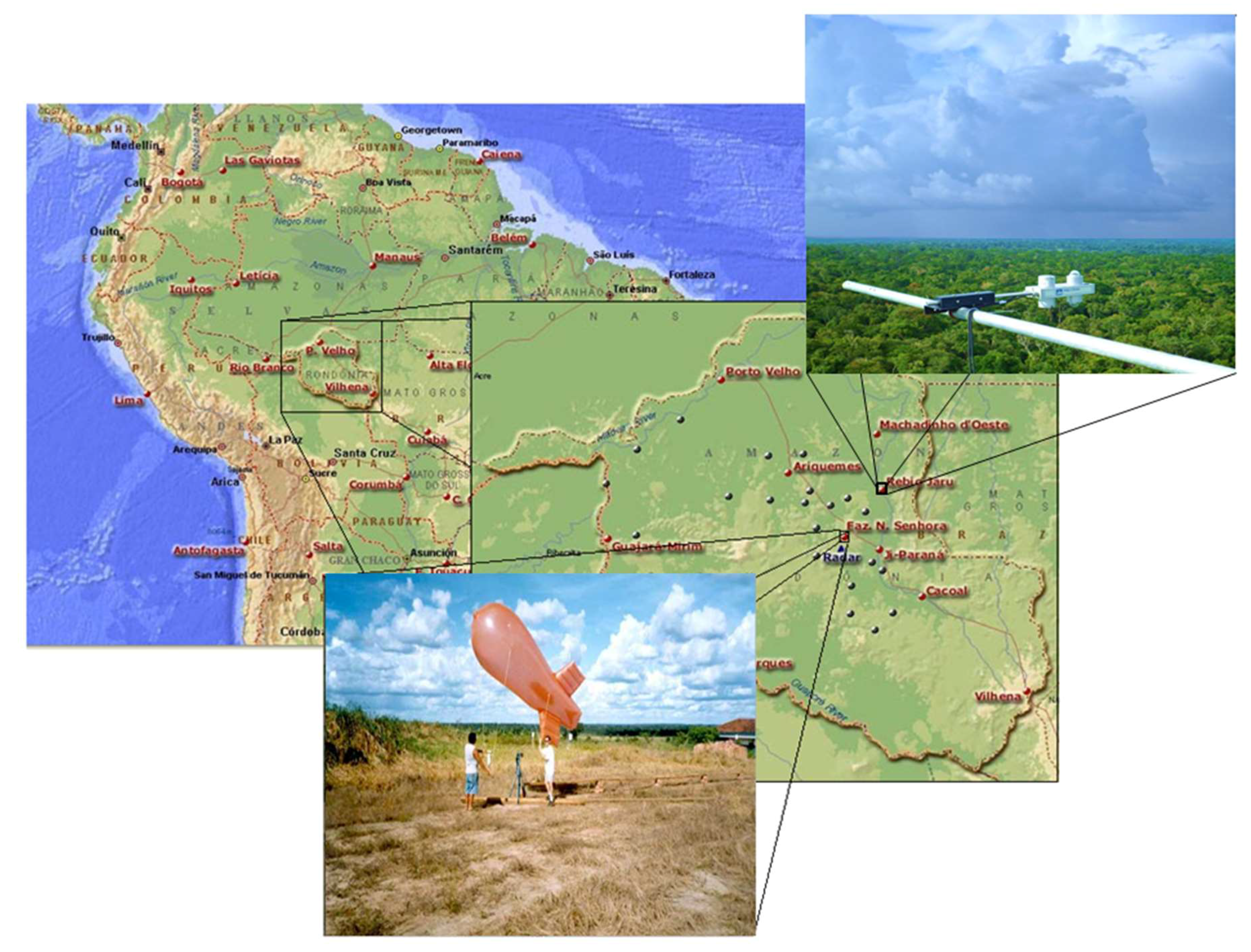
The areas chosen are representative of forest and grassland/pasture sites in Amazonia (more details in [20]) and they can be summarized as follows (Figure 1).
The forest area is located at the Biological Reserve of the Jaru River (hereafter FOR) at the coordinates 10°05’02” S, 61°55’55” W, located approximately 80 km northeast of Ji-Parana. This is an extensive area of 268,150 ha of almost intact upland rainforest, with average height of the canopy around 33 m, protected and preserved by the Brazilian Institute of the Environment (IBAMA).
The pasture area at Nossa Senhora Aparecida Farm (hereafter PAS) is at 10°46’25” S, 62°20’13” W, located 15 km from Ouro Preto d’Oeste village. It is a cattle breeding farm, where natural vegetation (forest) was completely removed and replaced with grass (Brachiaria).
At both sites, several field campaigns were carried out to obtain surface measurements and atmospheric conditions data. Among them, the data collected during the experiment “Rondônia Boundary Layer Experiment” (RBLE3) are often used to represent the dry season (hereafter, DRY), the measurement period for which occurred between 13 and 25 August 1994, covering the most intense phase of DRY [20]. These measurements consisted of radiosonde data, automatic weather station and turbulent flux data for surface data. The rainy season is hereafter referred to as WET.
2.2. The Parallelized LES Model (PALM)
The LES model was an implementation from Raasch and Schröter [21] and later improved by Maronga et al. [22]. The implemented version has a computational structure capable of optimum performance and high scalability to calculate architectures that are massively parallelized. PALM has been a very useful tool in various geophysical applications including the convective boundary layer [15,18,23,24], weakly stable boundary layer [25,26] and in neutral conditions [27,28].
Some general characteristics of PALM are that it is based on the Navier–Stokes equations, assuming the non-hydrostatic hypotheses, incompressible fluid and Boussinesq approximation. The equations for conservation of mass, energy and moisture are filtered on the grid size [29] and the molecular diffusion and radiation processes are generally neglected [21].
The subgrid-scale (SGS) turbulence is parameterized according to the [30] model which includes a predictive equation for turbulent kinetic energy of SGS (SGS-TKE), :
where I is local storage and II is advection of TKE in the horizontal averaged resolved-scale turbulent kinetic energy, III is the shear production (SP) term representing the conversion of mean flow kinetic energy to resolved-scale TKE, IV acts as either buoyant production or destruction (TP) term depending on the sign of the vertical heat flux, V is the net result of resolved-scale turbulent transport (TP) term, which represents the transport of resolved-scale kinetic energy by pressure fluctuations, and VI is the dissipation rate ε (VD) term [31,32]. Here, ui are the velocity components (u, v, w); xi are the Cartesian coordinates (x, y, z); ρ0 is the density of dry air; g is the gravitational acceleration; and θv = θ (1 + 0.608q − ql) is the virtual potential temperature with potential temperature θ, specific humidity q and liquid water mixing ratio ql. The variables with the double prime represent the SGS components and all the variables are filtered ones, but the overbar indicating filtered quantities is omitted except for the SGS flux terms for readability [28].
The SGS fluxes in the filtered equations (conservation of mass, energy, moisture and Equation (1)) are parameterized using the SGS eddy viscosity and diffusivity (subgrid-scale eddy coefficient for momentum) and (subgrid-scale eddy coefficient for scalar quantities) as in the sensible and latent heat equations
where is calculated by
where = 0.1 and . The SGS mixing length (l), in Equations (6) and (7), is calculated based on the vertical variation of virtual potential temperature [29]. The model equations are discretized by finite differences.
where z is the distance from the bottom. More information [21]
2.3. Domain Size Configuration
For the different conditions (in terms of surfaces and seasons), the simulations were generated for a domain of 10 km × 10 km × 5 km with a grid spacing of 50 m × 50 m × 50 m to reduce the computational demands. About 80 grid points were used in the vertical direction, stretched (Equation (8)) well above the capping inversion (3400 m) to further reduce the computational load [33].
where is the vertical grid space and sf is the stretch factor, which goes from 1.10 to 1.12.
The simulations had a cyclic boundary conditions, so that the same characteristic turbulences could be returned to the central point of the simulation, considering a feed of the same environment to the created domain.
To analyze the consistency of the grid spacing, two different grid spaces were tested for the simulations with the 15 August 1994 data, one with 25 m and other 50 m, for which the computational cost and an appropriate resolution for maximum analysis of model outputs determined the choice. To compare the results of the grid test simulation, the following statistical methods were used to compare each of the grids points of whole domain (N pairs of simulations and observations): the first was the Bias (Equation (9)), which is the simplest method, but it defines very clearly the systematic error (underestimation or overestimation), wherein and are, respectively, the results of simulations with 25 and 50 m grid spaces and N the number of data used in comparison. The second method was the Root-Mean-Square Error (RMSE), in Equation (10), a method commonly used due to its sensitivity to major differences between the compared series. To obtain congruence in the number of grid points and thus compare both the simulations, in S25m, the grid points were used every 50 m grid spacing. They can be any non-negative value and have the same unit of measurement of the series.
Using the metrics described, the results obtained (Table 1) for the variables of potential temperature (θ), specific moisture (q), vertical velocity (w), sensible () and latent () heat flux, turbulent kinetic energy (TKE) and friction velocity (u*) showed that there is no significant loss of information in the CBL simulation when a spacing of 50 m is selected, in addition to a reduced time gain (approximately 3 h per simulation). Thus, all simulations were performed with this spacing.
For the lateral boundary conditions, cyclic characteristics were used so that the local turbulent conditions could be more intensified.
2.4. Initialization and Forcing of the Simulations
To be representative of the seasons, simulations were performed with characteristic data of each period for one representative day. The days used were 15 August 1994 for the DRY period and 12 February 1999 for the WET period.
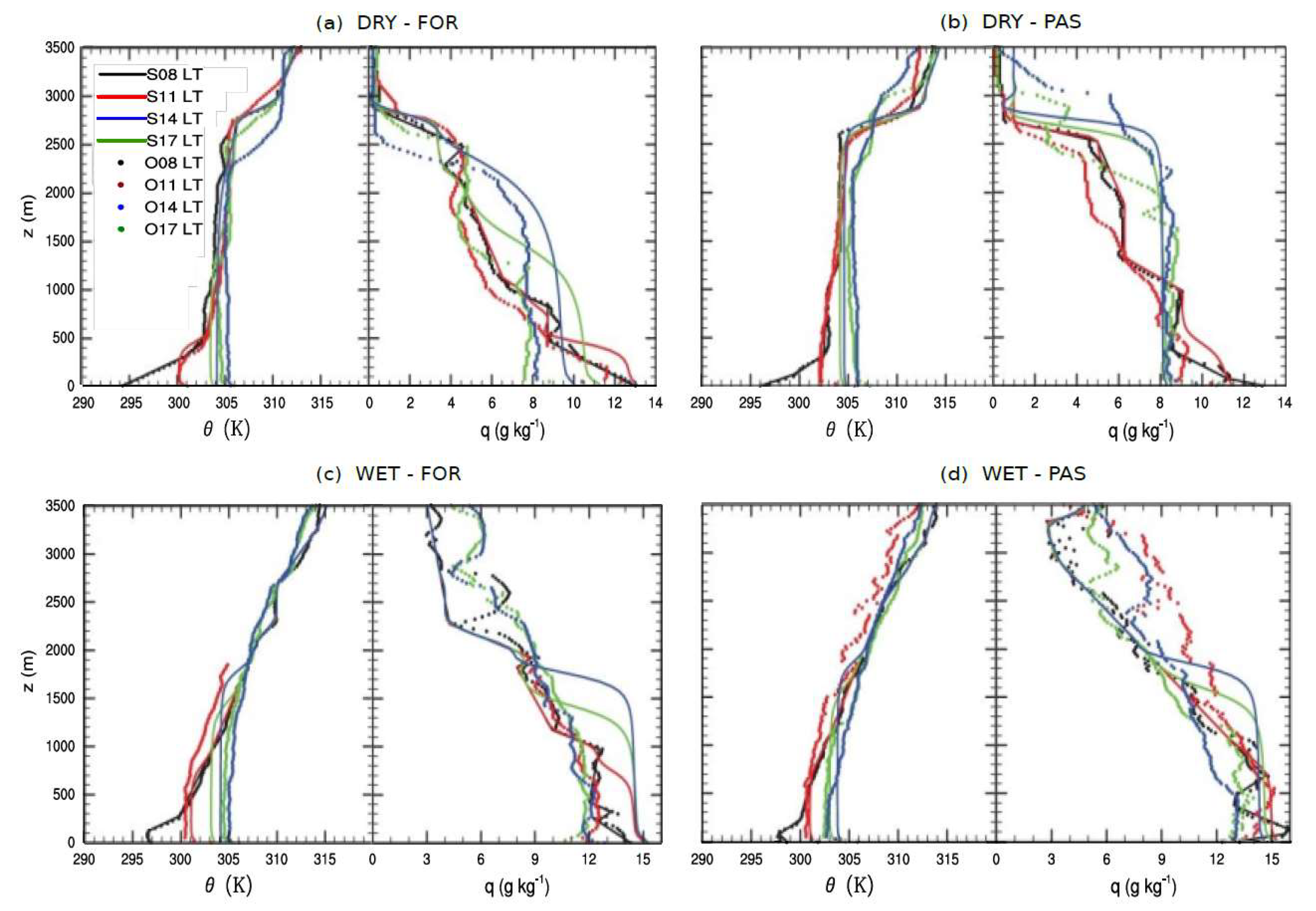
Since the interest was the convective systems, numerical simulations were started at 08:00 local time (LT), which is the time of the erosion of Nocturnal Boundary Layer and avoiding negatives fluxes prior to the sunrise. Besides surface temperature and humidity measurements, local characteristic profiles of potential temperature, specific humidity data (Figure 2) and wind components (not shown) were obtained by radiosondes launched in the experiments [20,34]. The comparisons were quite satisfactory for both sites, with values not exceeding 2.0 K of potential temperature vertically, while for specific humidity 2.0 g kg−1 for pasture and approximately 1.0 K and 4.0 g kg−1 for the forest.
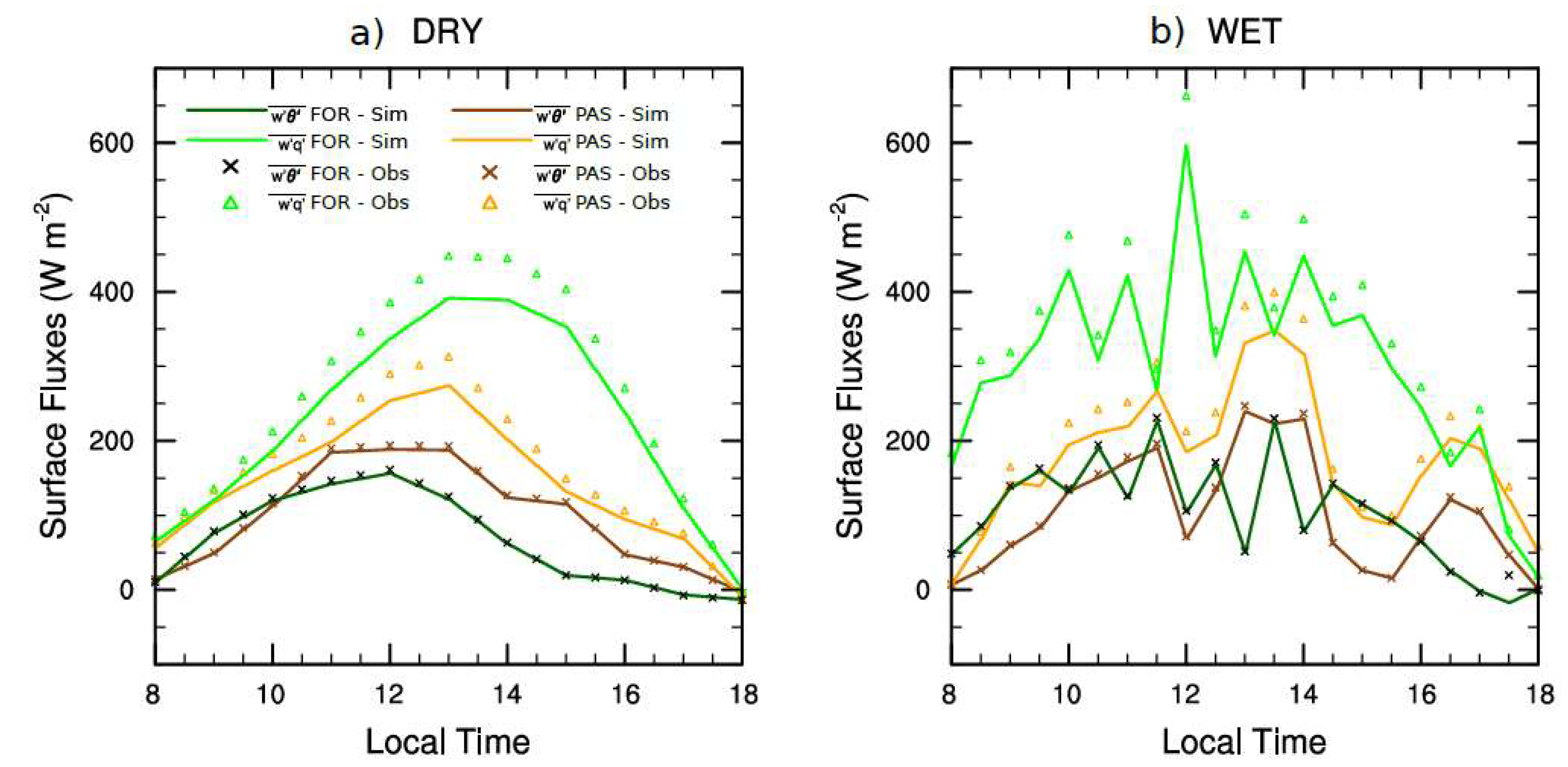
In addition, surface fluxes from local measurements using eddy covariance technique were used as driven (or given) surface sensible () and latent () heat flux for each respective land use type (Figure 3). Another characteristic used to distinguish each of the surfaces was the roughness length (z0), with the value of 3.03 m for the forest and 0.06 m for pasture, as suggested previously by Santos et al. [35].
2.5. Budget Turbulent Kinect Energy (TKE) Analysis
As suggested by Stull [36], TKE is one of the most important variables in micrometeorology due to its ability to measure the intensity of turbulence and describe processes through physical properties of Atmospheric Boundary Layer (ABL). Thus, with the goal of analyzing the budget of TKE (Equation (1)), neglecting subsidence, it represents: local storage or trend (LS); buoyance production or consumption (BP); shear production or loss (SP); turbulent transport of TKE (TT); pressure correlation (PC); and viscosity dissipation of TKE (VD). However, among the above terms, only BP, SP, TT and VD were analyzed, due to the interest in the convection produced by the amount of heat and mechanical production, and the transport and dissipation characteristics in each site and season.
3. Results and Discussion
3.1. Characteristics of Vertical Profiles and Surface Conditions
Temporal evolution of vertical profiles of potential temperatures and moisture, computed by horizontal mean of scalar values, over the experimental sites is plotted in Figure 2. The solid black line represents the initial data used to initialize the LES PALM model.
A cooler and drier condition was evident at early morning (08:00 LT) featuring a strong stability near the surface during the DRY for both sites. As an initial condition, there is a remaining and deeper NBL about 475 m height. The WET initialized thermal profiles by setting a CBL at 125 m. Because the stability at the surface formed at night condition is more intense during the dry periods, it is possible the CBL growth takes longer to start the diurnal convection. Another fact contributing to the difference in the initial profiles between seasons was the influence of higher humidity during the WET, which causes a strong stable stratification on both sites.
Due to the strong convection that takes place during the day, climatic elements such as rain can cease the growth of the CBL evolution and develop a new structure of mixed layer, keeping this pattern during the residual layer, even in the day after during the nocturnal boundary layer erosion. An example is the DRY case in the forest: at 08:00 LT, the profile presented a case in which two residual layers occur, one just above the NBL height at 450 m and the other one at the interface between PBL and the free atmosphere (around 2625 m).
The moisture profiles during DRY were drier and not so well mixed layer at high altitudes, with lower humidity in the CBL (except a relatively small neutral layer of 9.0 g kg−1) in the initial profile. At late afternoon (14:00–17:00 LT), the moisture profile showed neutral layers of approximately 8.0 g kg−1, with mixed layer height lower than those observed, possibly due to absence of large-scale horizontal advection. At the pasture site, there was greater presence of moisture at high altitudes; since convection contributes to the greater moisture through vertical transport near the surface, it does not show major differences between the observed and simulated altitudes of layers. With the lack of horizontal advection and the increase of moisture at the advent of the rainy season, mixing layers contain higher humidity on FOR and PAS sites, respectively, 12.0 and 13.5 g kg−1.
In general, with respect to the observed profiles, temperature profiles showed differences of about 1.0 K at both sites in WET, while the moisture profile in the DRY ranged 1.0–1.5 g kg−1.
Figure 3 shows the comparison of surface turbulent fluxes (sensible and latent heat) used as forcing boundary conditions. During the DRY period, the mean and (maximum of 448.4 W m−2) over FOR was higher (100.0 W m−2 and 130.0 W m−2, respectively) than over the PAS. For WET, the mean over the FOR was higher 337.3 W m−2 than over PAS, since this period has more moisture and easily produces a larger flow of moisture. In general, for WET was 40.0 W m−2 greater than during the DRY period and both surface turbulent fluxes ( and ) showed diurnal variation.
The profiles of the components of the sensible heat flux (), are: SGS (dashed line) and the resolved (line dash-dot) partitions of , and the sum of both terms, which is the total of (solid line). In the component profiles, the SGS of shows that the model was able to solve most of the vortices, except in locations where the presence of smaller vortices dominate. Analyzing the sensible heat flux profile of both sites and periods (DRY and WET) at 14:00 LT, the forest had the minimum negative heat flux in CBL height, while more intense thermal energy production on the surface was found in pasture. Other sensible heat flux characteristics are presented in Figure 4 as profile time series.
3.2. Sensible and Latent Heat Flux Time Evolution
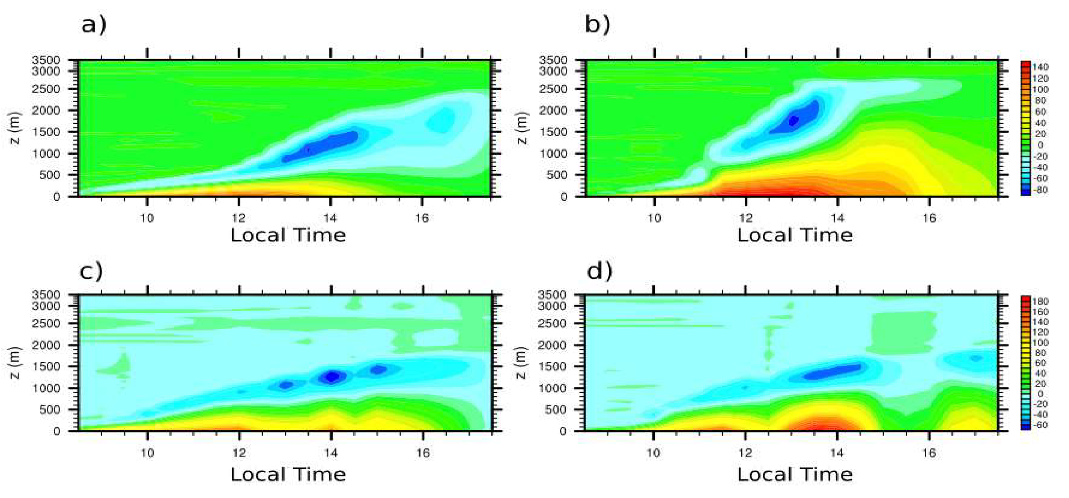
Figure 5 shows the time evolution of horizontal average values of sensible heat flux () profiles. During the DRY period (Figure 5a), the at forest is lower than the pasture and it becomes negative at the height 425 m at 12:30 LT. However, the most intense negative , of about −70.0 W m−2, persisted longer over FOR, between 13:00 LT and 14:30 LT. The at pasture (Figure 5b) showed high values (above 120 W m−2) between 11:30 and 14:00 LT. In the atmosphere, two vertical increase of positive occurred at 11:30 and 14:30 LT, causing more intense convection and providing a rapid growth of CBL height at these times. These abrupt growths with height, observed in the pasture, are connected to the residual layer from the previous day. The positive values of has a maximum at approximately 1600 m from 14:30 to 15:30 LT.
During WET, the , compared to DRY, presented in the forest site stronger values, while on the EZ level, DRY had more contribution of . In the pasture (Figure 5d), are closer to DRY, even with the pronounced variation due to clouds in WET. In WET, these values were very intense. Over forest (Figure 5c), the maximum sensible heat flux presented energies of 174.6 W m−2 at 11:30 LT in surface and −86.5 W m−2 on the ZE (at 14:00 LT), occurring 190 min after the maximum at surface. The physical reason to this difference of time is that the vertical movements at 14:00 LT are more intense, transporting more heat from the surface to the inner of CBL and also with stronger convective upper penetration movements (free atmosphere introducing heat to inside CBL). To the pasture, after a decay of the to 51.9 W m−2 at 12:00 LT, a maximum occurred with 231.0 W m−2, just before another decay (to 20.8 W m−2). From 14:30 to 16:00 LT occurred a very strong diminution of energy emitted by the surface (with maximum value of 15.9 W m−2), possibly due to the cloudy atmosphere, due to a value of zero of the in the EZ.
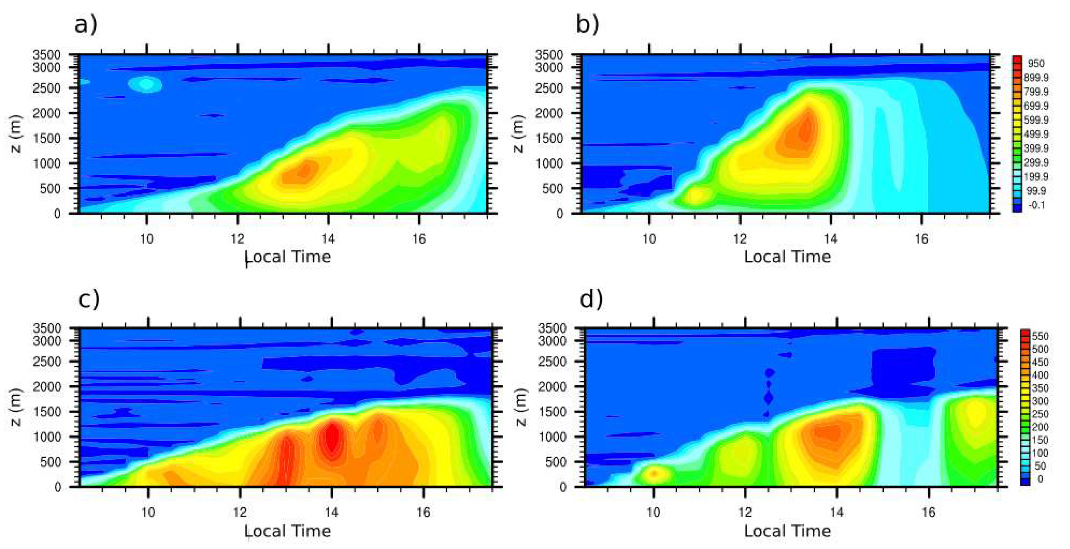
The in the DRY forest (Figure 6a) presented its maximum value at 13:30 LT with approximately 850.0 W m−2, just below the level of 1000.0 m. In the DRY pasture (Figure 6b), the maximum flow also occurred at 13:30 LT, with a value of 900.0 W m−2 at 1700.0 m. In the forest site, this flow proved to be more intense until the end of the day, while, in the pasture, shortly after the maximum, there was a reduction in the intensity of . In the WET period, over the forest was approximately 500.0 W m−2 between 13:00 and 14:00 LT, while at the top of the CBL its maximum was 687.5 W m−2 at 14:00 LT. Starting at 15:30 LT, there was a considerable reduction of until the end of the day. Over the WET pasture (Figure 7d), the EZ presented its maximum at 14:00 LT, as did the forest (Figure 6c), but with lower intensity (450.0 W m−2). After 14:00 LT, decreased until 102.6 W m-2 at the surface, caused by the strong reduction of flux in the entire CBL. After 15:30 LT, increased again, but did not surpass 300.0 W m−2 inside the CBL. This strong reduction of surface energy flux was also associated with the cloudy atmosphere.
3.3. TKE Budget
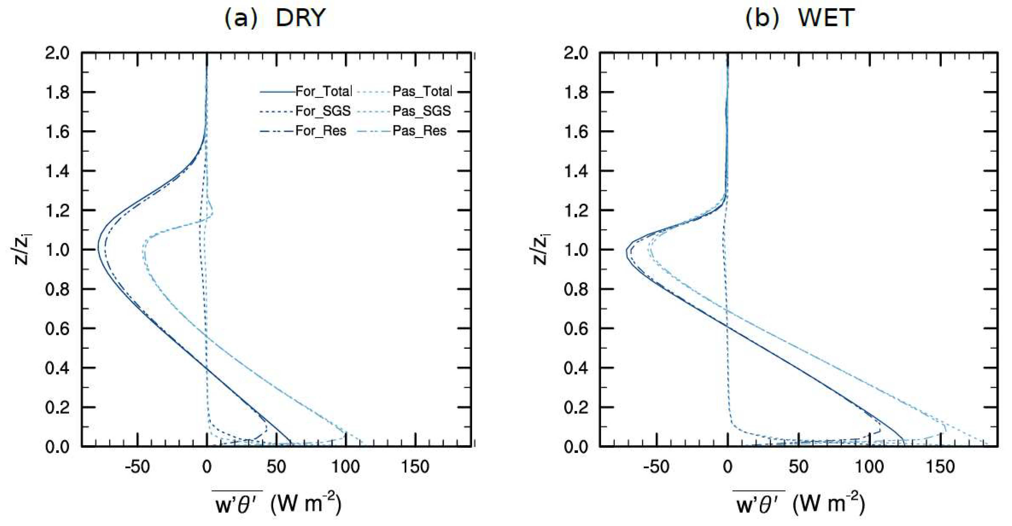
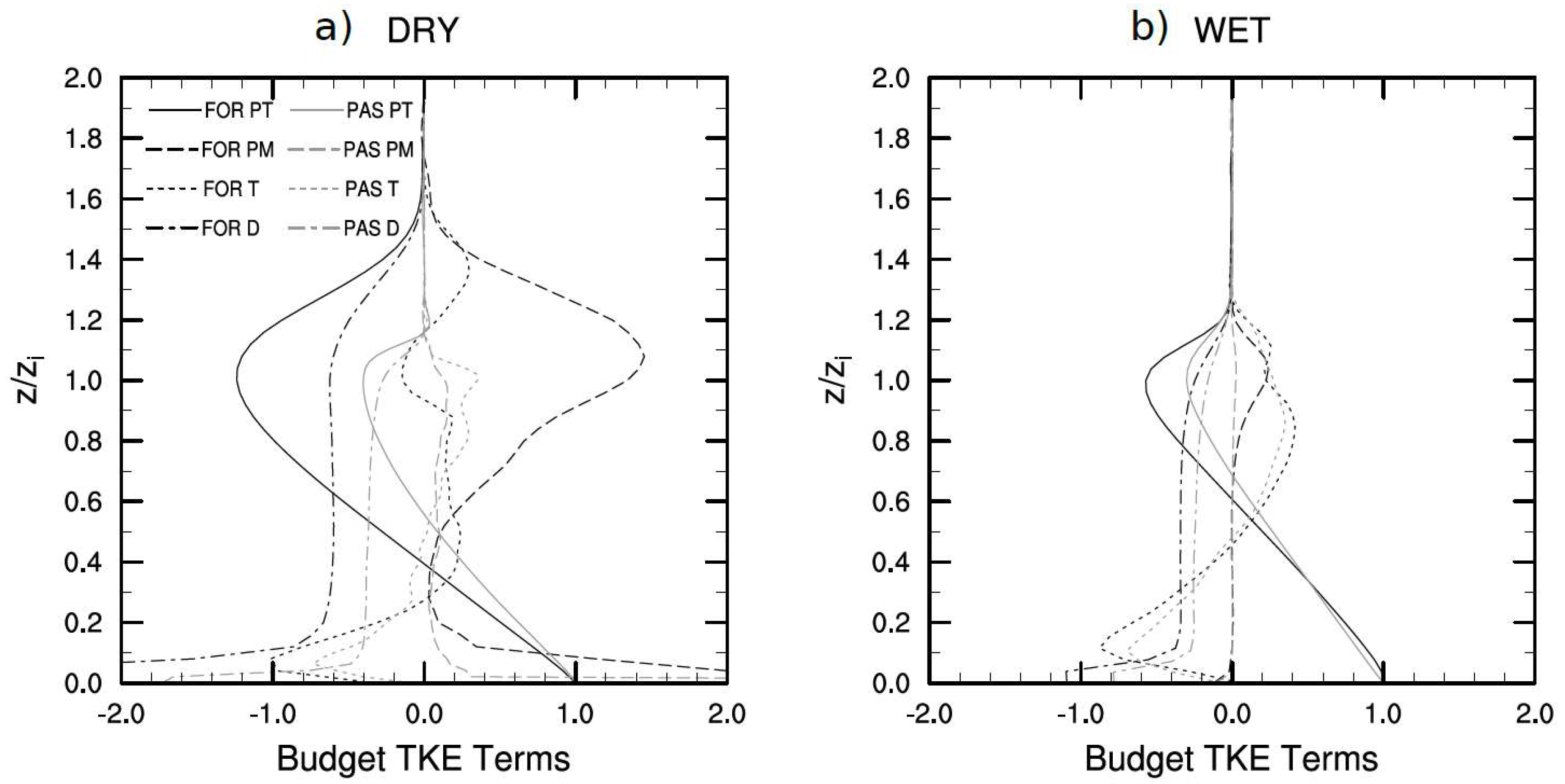
Estimated dimensionless TKE budget profiles are presented in Figure 7 for 14:00 LT, which represents the time of maximum convection activities. The terms are normalized by , in which represents the scale of convective velocity and the CBL height. The ratio has an order of 10−3 m2 s−3. The boundary layer height zi is defined as the height where the minimum negative value of heat flux is located, and the vertical scale of each profile is normalized by its own zi in each case.
Thermal or buoyancy production (TP) was very characteristic in both seasons, with a maximum at the surface and decreasing with height to the minimum at the top of the CBL (zi = 1.0). Over the FOR site, due to normalization with local conditions, during DRY (Figure 7a) and WET (Figure 7b) periods, more intense TP values occurred in the CBL height than in the PAS, in relation to surface values. However, during DRY, the characteristics of the profile were very distinct between the sites; while in the PAS the reduction of buoyancy production occurred quickly, at the FOR it extended up to about z = 1.5 zi. The energy at the top of CBL over the FOR interacts strongly with the entrainment zone in the DRY, showing the high buoyancy active contribution to the CBL on this surface.
The shear production (SP), in the DRY period, in the FOR surface had a very high order close to the surface with 2.2, decreasing until 0 by 0.3 zi deep inside the CBL and returning to produce more shear with an order of 1.4. The maximum SP that occurred in the PAS was at the surface with only 0.4. In WET period, PAS was almost totally absent and FOR presented a weak intensity at the top of the CBL top. This difference shows the very intense convection that was produced during the DRY, due to very high wind velocity.
The turbulent transport (TT) with the increase of convection tends to increase in intensity, but it is important to remember that it is not responsible for creating TKE, just for distributing it. Over FOR in DRY, TT near the surface was about −1.0, rapidly crossing 0.0 in z = 0.3zi determining the downward movement for the rest of the extension of the CBL. The downward maximum transport for this surface was 0.2 surpassing the CBL. With very strong ascendant but weak descendent movements a compensation occurred diminishing the ascendant layer. The PAS shows a transport near the surface of −0.7 and, after crossing the axis at approximately z = 0.5zi, remained below 0.4 until the top. In WET, both sites had a very similar TT, with more intense ascendant transportation due to the diurnal convection.
The viscosity dissipation (VD) shows a maximum near the surface especially when the winds have high magnitude, decreasing just above until disappearing above the CBL. In FOR in the DRY period, dissipation reached −3.2 with an average of −0.6 within the boundary layer. In the PAS, the dissipation rate was lower with a maximum at the surface of −1.7 and an average of −0.4 inside the layer. However, in the WET period, VD was less intense than in the DRY, since the SP was also weaker.
4. Conclusions
This work reveals significant analyses of the behavior of heat and humidity flows in the convective boundary layer associated with surface conditions by using a high resolution LES numerical model to better understand the patterns of turbulence and convection in different Amazonian sites. For DRY conditions, pasture observation produce a more highly heated surface than the forest, generating a more intense convection on the simulations eroding its NBL about 30 min before it occurs in the forest. In addition, due to this pasture heating, the final height of the CBL (2600 m) presents itself deeper than over the forest (2400 m).
Inputting the effective mixing of the boundary layer in a LES model, due to strong convection mainly in pastures, the latent heat flux shows a reduction and hence determines a greater amount of radiation is partitioned to the sensitive heat flux, which may grow in value and time. This sensible heat flux intensification with altitude feeds convection as well as the evolution of the CBL height. However, when a high availability of moisture occurs, as in forest environments and principally in wet periods, which contribute more moisture to the forest than the pasture, the latent heat flux is increased, regulating the amount of sensible heat and its growth in the atmosphere.
Based on TKE budget, the thermal production is the most important component for the energy process over both sites. The transport term is present with the same magnitude on all sites, and reaches 0 at about z = 0.5zi for WET, but it is more sensible to the intense convection of the DRY. In the forest, transport is the region with higher values, later in the day above 1.0. The dissipation responds with higher growth, especially in cases of the next largest mechanical production at the surface of the forest, reaching values up to −20.0. Considering the sites, the forest shows a higher thermal energy sink on top of the layer, but the production of mechanical energy, at the same time, helps in balancing dissipation.
Author Contributions
All authors contributed to the research and to the collaboration of this manuscript; T.N., processed and analyze the data, prepare the first draft of this paper, write up of the manuscript and contributed to its editing and finalization; G.F., analyze of the data, provided guidelines for the write up of the manuscript and contributed to its editing and finalization. S.R., process and analyze of the data.
Funding
This research was funded by CNPq through the PhD financial support of grant 140940/2014-6 and the doctorate sandwich program support of the program Science without Borders (241757/2012-6).
Acknowledgments
This project was developed with funding from CNPq.
Conflicts of Interest
The founding sponsors had no role in the design of the study; in the collection, analyses, or interpretation of data; in the writing of the manuscript, and in the decision to publish the results.
References
- Andreae, M.O.; Acevedo, O.C.; Araújo, A.; Artaxo, P.; Barbosa, C.G.G.; Barbosa, H.M.J.; Brito, J.; Carbone, S.; Chi, X.; Cintra, B.B.L.; et al. The Amazon Tall Tower Observatory (ATTO) in the remote Amazon Basin: Overview of first results from ecosystem ecology, meteorology, trace gas, and aerosol measurements. Atmos. Chem. Phys. Discuss. 2015, 15, 1599–11729. [Google Scholar] [CrossRef]
- Martin, S.T.; Artaxo, P.; Machado, L.; Manzi, A.O.; Souza, R.A.F.; Schumacher, C.; Wang, J.; Biscaro, T.; Brito, J.; Calheiros, A.; et al. The Green Ocean Amazon Experiment (GoAmazon2014/5) Observes Pollution Affecting Gases, Aerosols, Clouds, and Rainfall over the Rain Forest. Bull. Am. Meteorol. Soc. 2017, 98, 981–997. [Google Scholar] [CrossRef]
- Wendisch, M.; Pöschl, U.; Andreae, M.O.; Machado, L.A.; Albrecht, R.; Schlager, H.; Rosenfeld, D.; Martin, S.T.; Abdelmonem, A.; Afchine, A.; et al. The ACRIDICON-CHUVA campaign: Studying tropical deep convective clouds and precipitation over Amazonia using the new German research aircraft HALO. Bull. Am. Meteorol. Soc. 2016, 97, 1885–1908. [Google Scholar] [CrossRef]
- Oliveira, R.; Maggioni, V.; Vila, D.; Porcacchia, L. Using Satellite Error Modeling to Improve GPM-Level 3 Rainfall Estimates over the Central Amazon Region. Remote Sens. 2018, 10, 336. [Google Scholar] [CrossRef]
- Wali, M.K.; Lal, R. Amazonian Deforestation and Climate; Gash, J.H.C., Nobre, C.A., Roberts, J.M., Victoria, R.L., Eds.; John Wiley and Sons: New York, NY, USA, 1996. [Google Scholar]
- Nobre, A.D.; Oyama, M.D.; Oliveira, G.S. The Future Climate of Amazonia. 2014. Available online: http://www.ccst.inpe.br/o-futuro-climatico-da-amazonia-relatorio-de-avaliacao-cientifica-antonio-donato-nobre/ (accessed on 16 September 2018). (In Portuguese).
- De Souza, E.B.; Carmo, A.M.C.; Moares, B.C.; Nacif, A.; da Silva Ferreira, D.B.; Rocha, E.J.P.; Souza, P.J.D.O.P. Seasonal Precipitation over the Brazilian Legal Amazon: Climate Current and Future Projections Using REGCM4 Model. Available online: https://revistas.ufpr.br/revistaabclima/article/view/43711/28725 (accessed on 16 September 2018). (In Portuguese).
- Werth, D.; Avissar, R. The local and global effects of Amazon deforestation. J. Geophys. Res.Atmos. 2002, 107. [Google Scholar] [CrossRef] [Green Version]
- Marengo, J.A.; Tomasella, J.; Nobre, C.A. Climate change and water resources. Clim. Chang. 2017, 37, 7–23. [Google Scholar] [CrossRef]
- Salati, E.; Nobre, C.A. Possible climatic impacts of tropical deforestation. Clim. Chang. 1992, 19, 177–196. [Google Scholar] [CrossRef]
- Guimberteau, M.; Ciais, P.; Ducharne, A.; Boisier, J.P.; Dutra Aguiar, A.P.; Biemans, H.; De Deurwaerder, H.; Galbraith, D.; Kruijt, B.; Langerwisch, F.; et al. Impacts of future deforestation and climate change on the hydrology of the Amazon Basin: A multi-model analysis with a new set of land-cover change scenarios. Hydrol. Earth Syst. Sci. 2017, 21, 1455–1475. [Google Scholar] [CrossRef]
- Molion, L.C.B. Hydrology and water manegement in the humid tropics. In Amazonia Rainfall and Its Variability; Bonell, M., Hufschmidt, M.M., Gladwell, J.S., Eds.; Cambrigde University Press: Cambrigde, UK, 1993; pp. 99–111. [Google Scholar]
- Hastenrath, S. Annual cycle of upper air circulation and convective activity over the tropical Americas. J. Geophys. Res. 1997, 102, 4267–4274. [Google Scholar] [CrossRef] [Green Version]
- Horel, J.D.; Hahmann, A.N.; Geisler, J.E. An investigation of the annual cycle of convective activity over the tropical Americas. J. Clim. 1989, 2, 1388–1403. [Google Scholar] [CrossRef]
- Letzel, M.O.; Raasch, S. Large Eddy Simulation of Thermally Induced Oscillations in the Convective Boundary Layer. J. Atmos. Sci. 2003, 60, 2328–2341. [Google Scholar] [CrossRef]
- Patton, E.G.; Sullivan, P.P.; Moeng, C.H. The influence of idealized heterogeneity on wet and dry planetary boundary layers coupled to the land surface. J. Atmos. Sci. 2005, 62, 2078–2097. [Google Scholar] [CrossRef]
- Huang, H.Y.; Margulis, S.A. On the impact of surface heterogeneity on a realistic convective boundary layer. Water Resour. Res. 2009, 45. [Google Scholar] [CrossRef] [Green Version]
- Maronga, B.; Raasch, S. Large-eddy simulations of surface heterogeneity effects on the convective boundary layer during the LITFASS-2003 experiment. Bound. Lay. Meteorol. 2013, 146, 17–44. [Google Scholar] [CrossRef]
- Kurowski, M.J.; Teixeira, J. A scale-adaptive turbulent kinetic energy closure for the dry convective boundary layer. J. Atmos. Sci. 2018, 75, 675–690. [Google Scholar] [CrossRef]
- Fisch, G.; Tota, J.; Machado, L.A.T.; Silva Dias, M.A.F.; da F. Lyra, R.F.; Nobre, C.A.; Dolman, A.J.; Gash, J.H.C. The convective boundary layer over pasture and forest in Amazonia. Theor. Appl. Climatol. 2004, 78, 47–59. [Google Scholar] [CrossRef]
- Raasch, S.; Schröter, M. PALM-A large-eddy simulation model performing on massively parallel computers. Meteorol. Z. 2001, 10, 363–372. [Google Scholar] [CrossRef]
- Maronga, B.; Gryschka, M.; Heinze, R.; Hoffmann, F.; Kanani-Sühring, F.; Keck, M.; Ketelsen, K.; Letzel, M. O.; Sühring, M.; Raasch, S. The Parallelized Large-Eddy Simulation Model (PALM) version 4.0 for atmospheric and oceanic flows: Model formulation, recent developments, and future perspectives. Geosci. Model Dev. 2015, 8, 2515–2551. [Google Scholar] [CrossRef]
- Kanda, M.; Inagaki, A.; Letzel, M.; Raasch, S.; Watanabe, T. LES study of the energy imbalance problem with eddy covariance fluxes. Bound. Lay. Meteorol. 2004, 110, 381–404. [Google Scholar] [CrossRef]
- Raasch, S.; Franke, T. Structure and formation of dust devil–like vortices in the atmospheric boundary layer: A high-resolution numerical study. J. Geophys. Res. 2011, 116. [Google Scholar] [CrossRef] [Green Version]
- Beare, R.J.; Macvean, M.K.; Hostlag, A.A.M.; Cuxart, J.; Esau, I.; Golaz, J.-C.; Jimenez, M.A.; Khairoutdinov, M.; Kosovic, B.; Lewellen, D.; et al. An intercomparison of large-eddy simulations of the stable boundary layer. Bound. Lay. Meteorol. 2006, 118, 247–272. [Google Scholar] [CrossRef]
- Steinfeld, G.; Letzel, M.O.; Raasch, S.; Kanda, M.; Inagaki, A. Spatial representativeness of single tower measurements and the imbalance problem with eddy-covariance fluxes: results of a large-eddy simulation study. Bound. Lay. Meteorol. 2007, 123, 78–98. [Google Scholar] [CrossRef]
- Letzel, M.O.; Krane, M.; Raasch, S. High resolution urban large-eddy simulation studies from street canyon to neighbourhood scale. Atmos. Environ. 2008, 42, 8770–8784. [Google Scholar] [CrossRef]
- Maronga, B.; Reuder, J. On the Formulation and Universality of Monin–Obukhov Similarity Functions for Mean Gradients and Standard Deviations in the Unstable Surface Layer: Results from Surface-Layer-Resolving Large-Eddy Simulations. J. Atmos. Sci. 2017, 74, 989–1010. [Google Scholar] [CrossRef]
- Riechelmann, T.; Noh, Y.; Raasch, S. A new method for large-eddy simulations of clouds with Lagrangian droplets including the effects of turbulent collision. New J. Phys. 2012, 14. [Google Scholar] [CrossRef]
- Deardorff, J.W. Stratocumulus-capped mixed layers derived from a three-dimensional model. Bound. Lay. Meteorol. 1980, 18, 495–527. [Google Scholar] [CrossRef]
- Moeng, C.-H. A large-eddy-simulation model for the study of planetary boundary-layer turbulence. J. Atmos. Sci. 1984, 41, 2052–2062. [Google Scholar] [CrossRef]
- Mason, P.J. Large-eddy simulation: A critical review of the technique. Q. J. R. Meteorol. Soc. 1994, 120, 1–26. [Google Scholar] [CrossRef]
- de Rivas, K.E. On the use of nonuniform grids in finite-difference equations. J. Comput. Phys. 1972, 10, 202–210. [Google Scholar] [CrossRef]
- Silva Dias, M.; Petersen, W.; Dias, P.S.; Cifelli, R.; Betts, A.; Longo, M.; Gomes, A.; Fisch, G.; Lima, M.; Antonio, M.; Albrecht, R. A case study of convective organization into precipitating lines in the southwest amazon during the WETAMC and TRMM-LBA. J Geophys. Res. Atmos. 2002, 107. [Google Scholar] [CrossRef]
- Santos, R.D.; Fisch, G.; Dolman, A.J.; Waterloo, M. Modelagem da camada limite noturna (CLN) durante a época úmida na Amazônia, sob diferentes condições de desenvolvimento. Rev. Bras. Meteorol. 2007, 22, 387–407. (In Portuguese) [Google Scholar] [CrossRef] [Green Version]
- Stull, R.B. An Introduction to Boundary Layer Meteorology; Springer Science & Business Media: Berlin, Germany, 1988. [Google Scholar]
Figure 1.
Location of experimental sites. Source: http://www.lba.iag.usp.br.
Figure 1.
Location of experimental sites. Source: http://www.lba.iag.usp.br.

Figure 2.
Vertical profiles of potential temperature (θ) and specific humidity (q) in the course of the day for: FOR (a,c); and PAS (b,d) sites, during: DRY (a,b); and WET (c,d). The LES profiles are domain- and time-averaged (solid lines, 10-min mean), while sensor data are shown by dots.
Figure 2.
Vertical profiles of potential temperature (θ) and specific humidity (q) in the course of the day for: FOR (a,c); and PAS (b,d) sites, during: DRY (a,b); and WET (c,d). The LES profiles are domain- and time-averaged (solid lines, 10-min mean), while sensor data are shown by dots.

Figure 3.
Time series of the prescribed (marks) and LES simulation horizontal mean (solid lines) of surface sensible (a) and latent (b) heat fluxes.
Figure 3.
Time series of the prescribed (marks) and LES simulation horizontal mean (solid lines) of surface sensible (a) and latent (b) heat fluxes.

Figure 4.
Vertical profiles of turbulent thermal flux for FOR (Dark blue) and PAS (Light blue) sites at 14:00 LT for DRY (a) and WET (b) period. The LES profiles are domain- and time-averaged. The boundary layer height zi is defined as the height where the minimum negative value of buoyancy flux is located, and so the vertical scale of each profile is normalized by its own zi in each case.

Figure 5.
Time series of profiles of sensible heat flux over: FOR (a,c) ;and PAS (b,d) sites. During: DRY (a,b); and WET (c,d) seasons.
Figure 5.
Time series of profiles of sensible heat flux over: FOR (a,c) ;and PAS (b,d) sites. During: DRY (a,b); and WET (c,d) seasons.

Figure 6.
Time series of profiles of latent heat flux over: FOR (a,c); and PAS (b,d) sites. During: DRY (a,b); and WET (c,d) seasons.
Figure 6.
Time series of profiles of latent heat flux over: FOR (a,c); and PAS (b,d) sites. During: DRY (a,b); and WET (c,d) seasons.

Figure 7.
Budget of turbulent kinetic energy (normalized by w*/Zi) over FOR (dark grey) and PAS (light grey) surfaces in DRY and WET.
Figure 7.
Budget of turbulent kinetic energy (normalized by w*/Zi) over FOR (dark grey) and PAS (light grey) surfaces in DRY and WET.


Table 1.
Statistical comparison of BIAS and RMSE between 25 m and 50 m grid spacings.
| Θ | q | w | TKE | u∗ | |||
|---|---|---|---|---|---|---|---|
| (Κ) | (g kg−1) | (cm s−1) | (K m s−1) | (kg kg−1 m s−1) | (m2 s−2) | (m s−1) | |
| Bias | −0.15 | 0.22 | 0.02 | 1.11 × 10⁻⁷ | 1.87 × 10⁻¹³ | −2.33 | −0.01 |
| RMSE | 5.17 × 10⁻⁴ | 0.52 | 0.05 | 1.52 × 10⁻⁶ | 2.6 × 10⁻¹² | −2.35 | 0.02 |
© 2018 by the authors. Licensee MDPI, Basel, Switzerland. This article is an open access article distributed under the terms and conditions of the Creative Commons Attribution (CC BY) license (http://creativecommons.org/licenses/by/4.0/).
Share and Cite
MDPI and ACS Style
Neves, T.; Fisch, G.; Raasch, S. Local Convection and Turbulence in the Amazonia Using Large Eddy Simulation Model. Atmosphere 2018, 9, 399. https://doi.org/10.3390/atmos9100399
AMA Style
Neves T, Fisch G, Raasch S. Local Convection and Turbulence in the Amazonia Using Large Eddy Simulation Model. Atmosphere. 2018; 9(10):399. https://doi.org/10.3390/atmos9100399
Chicago/Turabian StyleNeves, Theomar, Gilberto Fisch, and Siegfried Raasch. 2018. "Local Convection and Turbulence in the Amazonia Using Large Eddy Simulation Model" Atmosphere 9, no. 10: 399. https://doi.org/10.3390/atmos9100399
Note that from the first issue of 2016, this journal uses article numbers instead of page numbers. See further details here.