Thermochemical Non-Equilibrium in Thermal Plasmas


1
CORIA, UMR CNRS 6614, Normandie Université, 76801 St-Etienne du Rouvray, France
2
CNES, French Spatial Agency, 31400 Toulouse, France
*
Author to whom correspondence should be addressed.
Atoms 2019, 7(1), 5; https://doi.org/10.3390/atoms7010005
Submission received: 30 November 2018
/
Revised: 24 December 2018
/
Accepted: 25 December 2018
/
Published: 1 January 2019
(This article belongs to the Special Issue SPIG2018)
Abstract
:In this paper, we analyze the departure from equilibrium in two specific types of thermal plasmas. The first type deals with the plasma produced during the atmospheric entry of a spatial vehicle in the upper layers of an atmosphere, specifically the one of Mars. The second type concerns the plasma produced during the laser-matter interaction above the breakdown threshold on a metallic sample. We successively describe the situation and give the way along which modeling tools are elaborated by avoiding any assumption on the thermochemical equilibrium. The key of the approach is to consider the excited states of the different species as independent species. Therefore, they obey to conservation equations involving collisional-radiative contributions related to the other excited states. These contributions are in part due to the influence of electrons and heavy particles having a different translation temperature. This ‘state-to-state’ approach then enables the verification of the excitation equilibrium by analyzing Boltzmann plots. This approach leads finally to a thorough analysis of the progressive coupling until the equilibrium asymptotically observed.
1. Introduction
The question of the existence of the thermodynamic equilibrium is crucial in plasma physics [1,2]. Indeed, since the energy can be freely distributed over the different excited states, radiation can be easily emitted, which leads to discrepancies in terms of population with respect to the Boltzmann distribution. In addition, ionization or recombination deals with excited states whose population density cannot be easily estimated. Moreover, temporary species, whose density would be negligible in case of thermodynamic equilibrium, can be formed and can have a significant influence on the behavior of the plasma.
Many experimental and theoretical works have been devoted to plasma physics and the main objective of this communication is not to overview the field. This would be necessarily incomplete. Conversely, it is more interesting to focus our attention on unusual situations to enrich the analysis. The CORIA laboratory in France, with the collaboration of the French spatial agency CNES (Centre National d’Etudes Spatiales), works on plasmas produced during the planetary atmospheric entry of spatial vehicles. The CORIA laboratory works also on laser-induced plasmas in the framework of the multi-elemental composition determination based on the laser-induced breakdown spectroscopy (LIBS) technique with the CEA (Commissariat à l’Energie Atomique et aux Energies Alternatives). In these two cases, the plasma can depart significantly from thermodynamic equilibrium, and analyzing this departure helps to enlarge our understanding of the global behavior of the plasmas. This is why we propose in the present communication to focus our attention on these situations.
As a result, the structure of the communication is separated in two main parts. The first part is dedicated to planetary atmospheric entry plasmas and the second part is devoted to the laser-induced plasmas. In each part, the context is given as well as the main features of the related plasmas. Then, tools are presented to characterize the plasmas formed using relevant models.
2. Planetary Atmospheric Entry Plasmas
2.1. Context
Due to gravity, the speed of bodies coming from space can be high. Typically, this speed reaches several . When the body approaches a planet having an atmosphere, the penetration of its upper layers generates the formation of a shock layer by compression around the forward part of the body [3,4]. The temperature in this layer increases significantly at levels reaching easily several . A gas to plasma transition takes place in the shock layer and leads to a strong heat transfer to the surface of the body. This heat transfer can be high enough to increase its surface temperature beyond the melting point and to cause the destruction of this surface. In the case of a manned-controlled mission, from the technological point of view, the covering of the spatial vehicle external surface by a thermal protection system (TPS) based on the use of ceramic materials is therefore mandatory.
Literature reports many entries in the Earth [5] or in the Mars [6] atmospheres. They can be controlled in the case of the flight of spatial vehicles, or totally uncontrolled in the case of natural bodies. For Earth, the human missions are well controlled and are particularly illustrated by the supplying of the International Space Station (ISS) at an altitude of . One of the most impressive events of natural entry took place on 15th February 2013 when a meteorite crossed the sky of the city of Chelyabinsk in Russia before to crash on the ground. Many cameras filmed this event, which clearly put in evidence the strong level of temperature reached in the shock layer through the strong emitted radiance.
2.2. Inside the Shock Layer
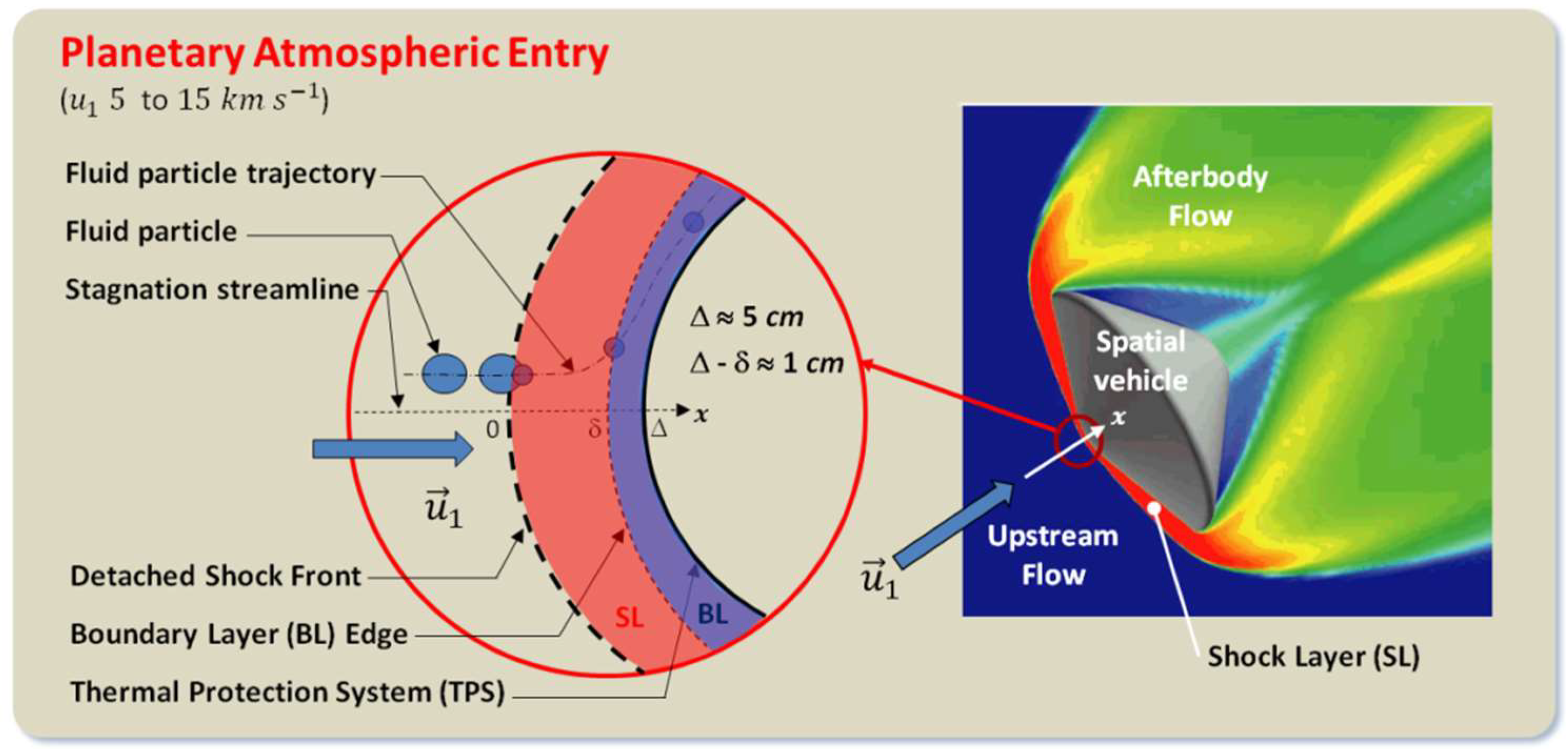
Figure 1 illustrates the production of the shock layer (thickness of in order of magnitude) due to the fast external gas motion relative to the surface of a spatial vehicle. In particular, a fluid particle is followed along its trajectory. Entering the shock layer by crossing the detached shock front, its volume is strongly decreased due to the increase in pressure. As a result, the temperature increases and provokes chemical non-equilibrium leading to the global dissociation and ionization of the flow. If the trajectory is close to the stagnation streamline, the fluid particle enters the boundary layer in which the plasma flow gives energy to the body surface (in ). In this part, the temperature decreases approaching the body, which leads to significant gradients. In this region, whose typical thickness is , the recombination occurs. Consequently, these recombined species will interact with the TPS.
The thickness of these layers is pretty low. In addition, although the speed is decreased at the crossing of the shock front, the speed remains sufficiently high in the shock layer to prevent local thermodynamic equilibrium. Indeed, the three Damkhöler numbers—, , and —defined as
are not much higher than unity. Since the speed is high, the value of the characteristic time scale for convection is weak. The time scale for the collisional-radiative source term of the species is of the same order of magnitude, which leads to a Damkhöler number close to unity. The flow is therefore out of chemical equilibrium (in case of chemical equilibrium, ) and not frozen (in case of frozen flow, ). The time scale to reach a Maxwell–Boltzmann distribution for the translation (of electrons or heavy species) is much shorter than , which leads to . As a result, the translation equilibrium is reached. However, the coupling between electrons and heavy species is difficult: the time scale of coupling is then higher than and the third Damkhöler number is therefore lower than unity. Thus, the flow is out of thermal and chemical equilibrium, in other words the flow is in thermochemical non-equilibrium.
These features have important consequences on the heat transfer to the surface. The presence of species not formed in case of chemical equilibrium and the spectral radiance emitted by the plasma lead to additional contributions. The local parietal heat flux density is then given by
and can easily exceed . In Equation (2), the first part of the right side refers to the influence of translation and internal modes transfer, the second part to parietal catalysis and the third part to radiation. is the thermal conductivity for the mode whose temperature is , is the recombination probability for species , is the energy accommodation coefficient, is the spectral absorptivity, is the spectral transmittivity along , is the distance with the elementary volume , is the angle with respect to the normal vector and is the spectral emission coefficient.
The estimation of the wall heat flux density requires a detailed knowledge of the plasma upstream the boundary layer. The CORIA laboratory develops models to go deeper in its understanding. In the upcoming section, we focus our attention on the work dedicated to the EXOMARS mission.
2.3. The EXOMARS Mission
Recently, the European Space Agency (ESA) in cooperation with the Russian Space Agency (ROSCOSMOS) managed the EXOMARS mission whose first step was the landing on the ground of Mars of a rover on board of the Schiaparelli lander on 19th October 2016 [7]. The TPS of the lander was equipped with sensors called ICOTOM embedded in the COMARS+ housing whose role was to provide information on the radiative signature in the infrared part of the spectrum [8]. The related radiation is due to the production of hot CO2 and CO during the entry in the Martian atmosphere and corresponds to the radiative contribution to in Equation (2) in the afterbody flow. This atmosphere is indeed mainly composed of CO2 (95.97%), Ar (1.93%), and N2 (1.89%). Crossing the shock front, this mixture is then put at high temperature and pressure. The composition then changes since this composition does not correspond to chemical equilibrium. To estimate chemical relaxation time scales of this mixture, we have developed models able to show how this relaxation occurs in a typical situation. Since the composition of the upstream atmosphere is well known, we focus our attention on the shock crossing when the heat transfer to the TPS is maximum, therefore over the first centimeters after the shock. This situation of “peak heating” corresponds to an altitude of [9].
2.4. Modeling of the Shock Front Crossing
Since the excitation equilibrium condition is not systematically fulfilled, the modeling is based on the solution of the excited states population density balance equation written as
assuming negligible the diffusion phenomena within the post-shock flow at steady-state. In Equation (3), is the mass fraction of the species on its excited state whose mass is . The collisional-radiative term results from the influence of all the elementary inelastic/superelastic processes enabling a change in the population density . The mass flow density is written .
Equation (3) is coupled with the momentum balance equation
whose pressure is calculated by the Dalton law assuming a perfect gas-like behavior.
Equations (3) and (4) are finally coupled with the energy balance of heavy particles
and of electrons
These equations must be considered separately because the energy per unit volume and for heavies and electrons depend on the heavy species temperature and on the electron temperature , respectively. The Dalton law is obvious and the mass density results from the summation of the contributions of heavy species and electrons . Inelastic/superelastic elementary processes are considered through the term while the term results from the influence of the radiative recombination whose emission coefficient is . The spontaneous emission is related to the emission coefficient .
The complexity of the upstream flow composed of CO2, N2, and Ar induces a very complex chemistry past the shock front. To be relevant, this chemistry must include enough species that can be formed in the post-shock conditions based on C, O, and N atoms. The pressure conditions are insufficient to produce Ar2+ dimers. The species taken into account in the resulting CoRaM-MARS collisional-radiative model are listed in Table 1. This list involves 21 species and electrons, 1600 excited vibrational and electronic excited states. All the vibrational states of the molecular electronic ground states are taken into account to reproduce realistically the global dissociation processes.
When the mixture crosses the shock front, a drastic reduction of the mean free path takes place due to the strong increase in mass density . The typical thickness of a shock front is of several mean free paths. In a first approximation, we can consider this increase so rapid that this corresponds to a discontinuity. The Rankine–Hugoniot jump conditions at the shock front can then be used, where the chemistry is frozen. Electron temperature remains unchanged because the rare electrons are not perturbed by the shock front. Indeed, due to their very weak mass, the electrons are in a quite subsonic flow regime. Heavy species temperature is conversely strongly increased at a level incompatible with the upstream chemical conditions. Chemistry then starts, which modifies the composition as a result of the elementary processes, first due to heavy species impact, the electron density being too weak. When is high enough, the elementary processes are driven by the electron-induced collisions. These elementary processes are collisional (vibrational excitation, dissociation, electronic excitation, ionization, excitation transfer, neutral and charge exchanges, and backward processes driven by the detailed balance principle), radiative (spontaneous emission) or mixt (radiative recombination, photo-ionization, self-absorption). This underlying chemistry represents a set of around elementary reactions [10].
2.5. Some Results
Due to the upstream conditions in terms of pressure, temperature and speed relative to the spatial vehicle when the peak heating occurs, the crossing of the shock front in induces high values of temperature and pressure. Table 2 gives the jump conditions. We can see that the temperature is clearly incompatible with an insignificant dissociation degree for CO2. The collision frequency and the energy available in the collisions then start the chemistry.
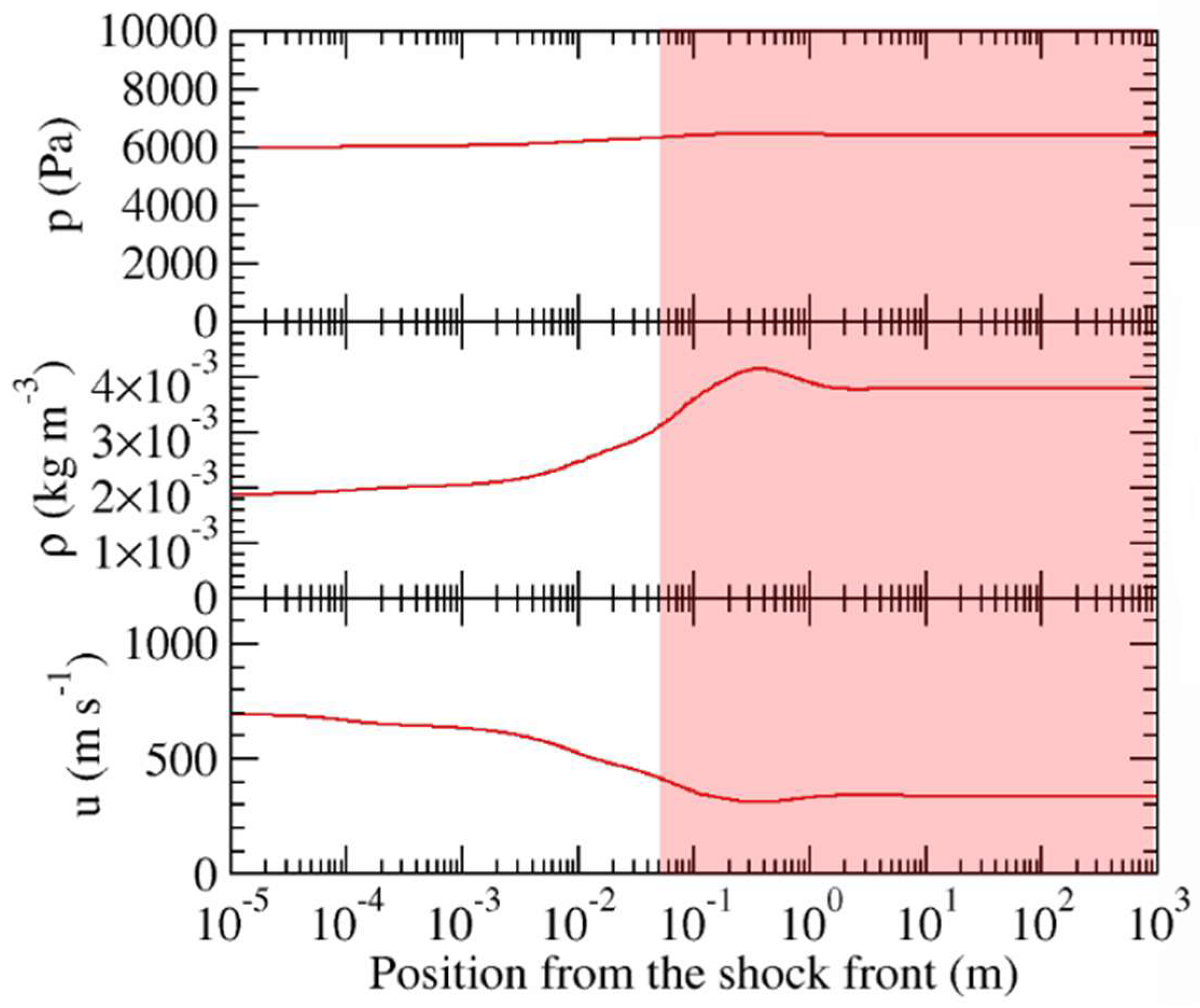
Figure 2 displays the resulting distribution of the aerodynamic variables (pressure, mass density, and speed). Even if Equations (3)–(6) are available only in the region where the diffusion phenomena are negligible (typically before the boundary layer, for ), we have displayed all the relaxation as we could observe in shock tubes, to see the final convergence of the flow. Since the boundary layer starts at , only the first centimeters of the solution displayed on Figure 1 are relevant with respect to the real situation.
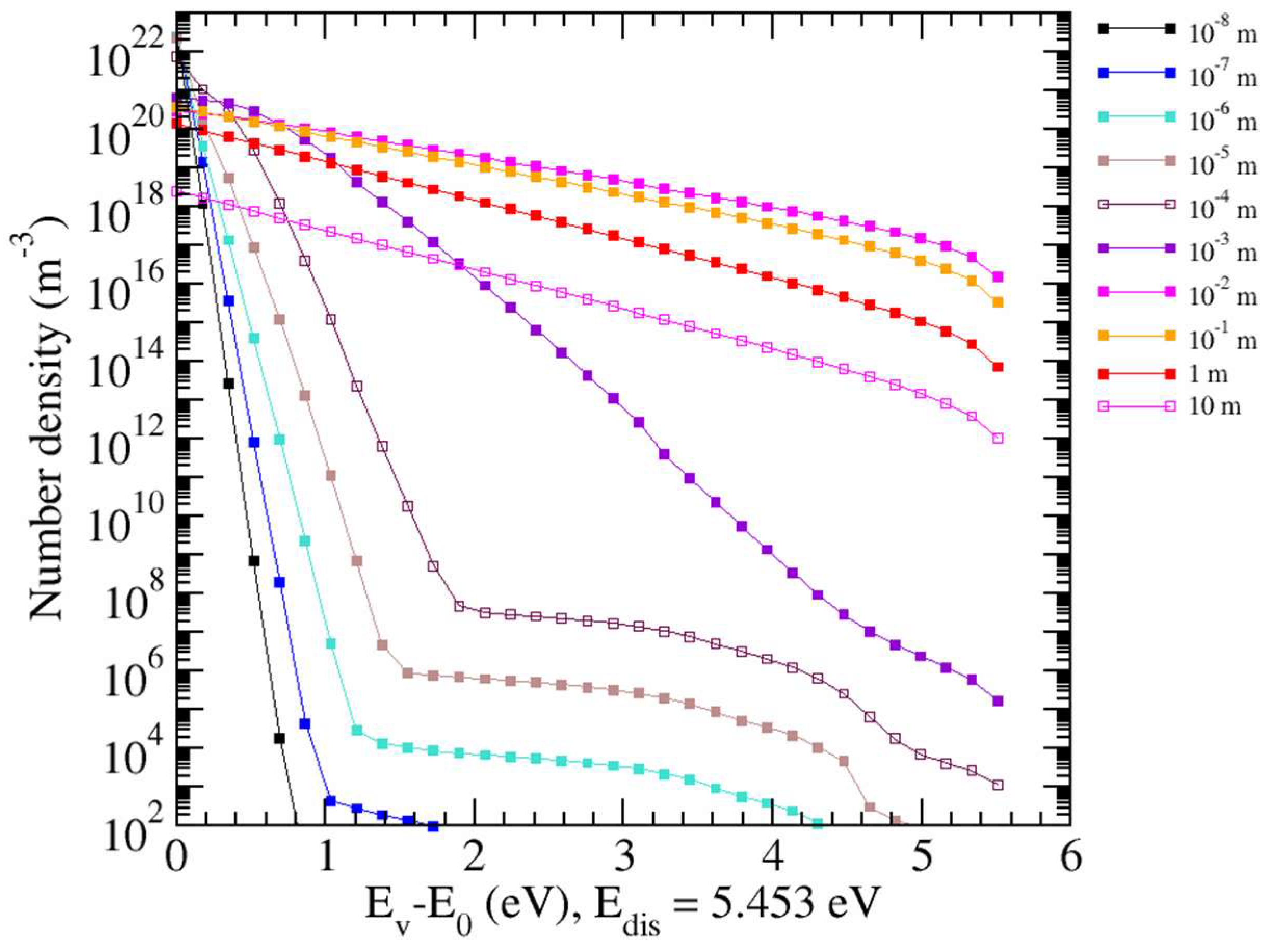
Figure 2 clearly shows that the relaxation is still in progress at . This is also clearly shown by Figure 3 where the Boltzmann plots of the CO2() vibrational states is displayed as a function of the position from the shock front. The vibrational distribution is far from being linear, that reveals a departure from vibrational excitation equilibrium.
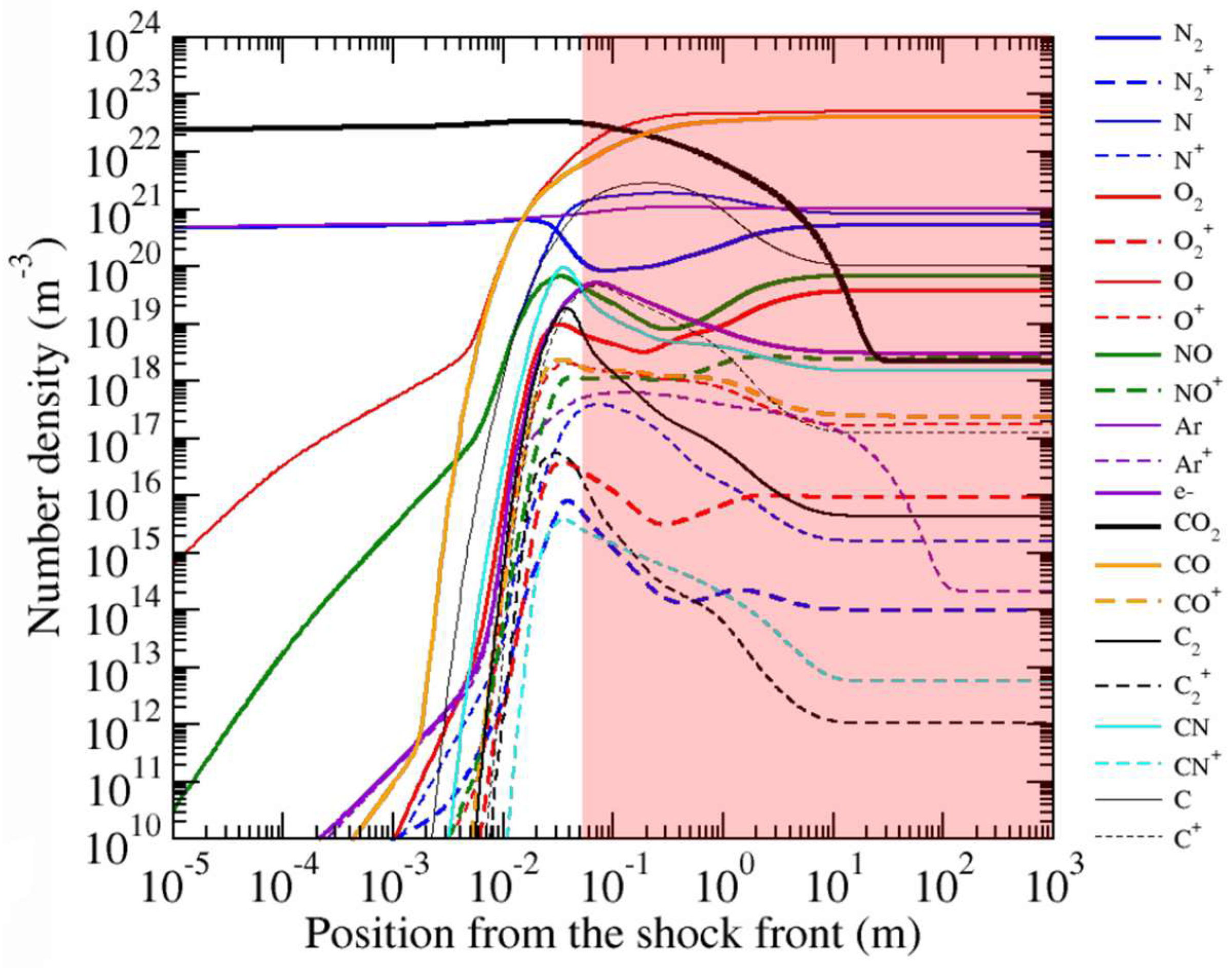
The way to the dissociation is mainly driven by the excited vibrational states close to the dissociation limit [11]. As a result, these distributions prove that the dissociation equilibrium is not reached. Indeed, the distribution of the species number densities displayed on Figure 4 illustrates the current global dissociation process. The formation of CO and O resulting from the dissociation of CO2 is clearly observed. The dissociation degree is close to 0.01 at after the shock front and to 0.35 at . Molecular and atomic ions start to be produced just after the dissociation of CO2. A maximum electron density of is obtained at a location close to and corresponds to an ionization degree of . Even if this amount seems to be rather small, the electron density is nevertheless high enough to significantly influence the chemistry. Indeed, due to their weak mass, the efficiency of electrons in terms of inelastic/superelastic collisions is much stronger than the one of the heavy particles. However, this influence is reduced since the electron temperature is lower than the heavy particle temperature .
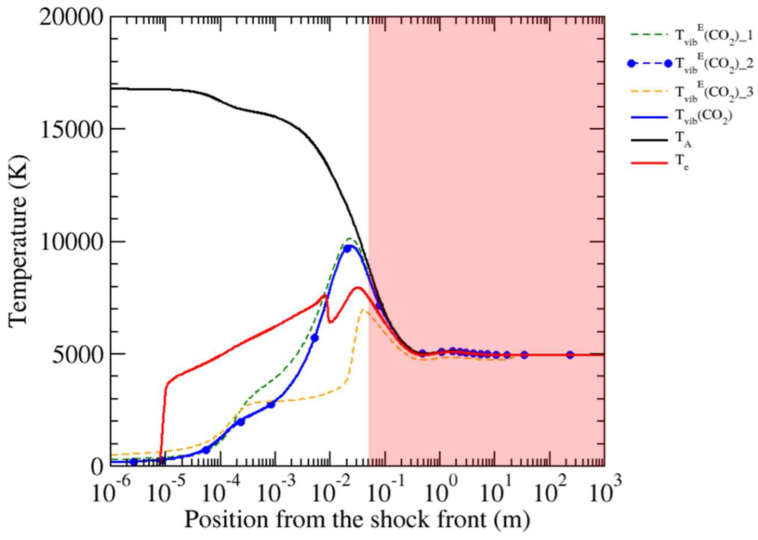
Figure 5 illustrates the distribution of temperatures. and have been plotted. We have also plotted the distribution of the post-processed values of the energy-dependent vibrational temperature for each vibrational mode of CO2 resulting from our vibrational state-to-state approach. The total energy-dependent vibrational temperature has been also determined.
This energy-dependent vibrational temperature for a mode is derived from the vibrational energy per unit volume by the equation
In the case of the mean vibrational temperature , the summations of Equation (7) are extended to the vibrational modes.
On Figure 5, we can see the progressive coupling between the three modes with the distance from the shock front. No one is perfectly coupled with the translation temperature of electrons or heavy particles before the limit of the boundary layer. We can also observe that the temperature departure between the first (symmetric stretching) mode and the second (bending) mode is pretty low. This is mainly due to the Fermi resonance resulting from the energy diagram. The quasi resonance between the related states leads to easy excitation transfer between them. The third (asymmetric stretching) mode is more difficult to excite and remains at temperature rather low. It is particularly interesting to see that, despite the thermal non-equilibrium between these states, they do not contribute in the same way to the mean vibrational temperature. Indeed, Figure 5 shows that this temperature follows the vibrational temperature of the second (bending) mode. This is mainly due to the degeneracy of the states of the second vibrational mode. While the first and third vibrational modes are not degenerated, the second mode presents a degeneracy equal to resulting from the rotational motion induced by the bending of the molecule. One finds further molecules per unit volume in the related states and the global vibrational temperature follows the one of this mode.
The differences observed on Figure 5 between the vibrational modes of CO2 are the result of the thermal non-equilibrium and of the efficiency of electrons and heavies in terms of collisions. In addition, the electrons and heavy particles dynamics is deeply different since electrons are produced and heated behind the shock front while the heavies leave their energy along the flow where the global dissociation process takes place. This corresponds therefore to a strong non-equilibrium situation. This situation relaxes over typical length scales longer than the shock layer thickness as illustrated by Figure 5. The thermal non-equilibrium would be resorbed around from the shock front in case of infinite shock layer thickness. Since , we conclude to a limit of the boundary layer departing from thermal equilibrium. This conclusion departs from the usual one considered for the case of Earth atmospheric entries [12].
3. Laser-Induced Plasmas
3.1. Context
The laser-induced plasmas correspond also to an interesting situation where thermodynamic non-equilibrium plays an important role. These plasmas are produced when a (typically nanosecond) laser pulse reaches a sample at a spectral irradiance of higher than the breakdown threshold (see Figure 6). The absorption of the laser energy leads to a strong increase in the local temperature of the sample at values (of the order of several ) exceeding largely the conditions of a phase change. A plasma is indeed produced whose pressure is initially very high (of the order of several ) with respect to the background gas one. The produced plasma then expands according to a hypersonic regime (the Mach number can reach values of the order of ), produces a shock wave propagating in the background gas and cools mainly owing to the radiative losses. This leads to a physical object having lifetimes of the order of several .
The atoms and ions composing the plasma are initially inside the sample. Once the plasma relaxed, a crater is formed where the laser pulse reached the sample. The radiative signature of the plasma can therefore give valuable information about the composition of the sample. This explains why this laser–matter interaction is at the basis of the laser-induced breakdown spectroscopy (LIBS) technique to determine the multi-elemental composition of samples. Measuring the spectral radiance of relevant lines, it is possible to derive the relative population of the different species if thermochemical equilibrium conditions are fulfilled [13].
3.2. Possible Non-Equilibrium Situation
The pulse duration plays an important role on the interaction. In the case of ultrashort ( or ) pulses, the laser energy is directly deposited within the material and leads to thermal non-equilibrium because electrons and heavies have not enough time to be coupled. In the case of laser pulses, the end of the pulse is absorbed by the plasma in expansion with a good coupling between electrons and heavies. In addition, thermal effects due to heat diffusion within the material can be observed for laser pulses and can produce micro-droplets, contrary to the case of the ultrashort laser pulses where nanoparticles can be observed. This explains the use of laser sources for the micromachining devices.
In terms of ablation precision, it is therefore better to use ultrashort laser pulses. According to the experimental setup used, a nominal ablation rate as low as some can be reached. This means that the matter forming the laser-induced plasma is in low amount. Typically, experiments are performed by accumulating signals over a tenth of pulses. Then the net minimum ablation rate is of . A depth profiling of the sample is therefore possible if the spectral radiance of the relevant lines is high enough to provide significant results. We consider only picosecond laser pulses in the upcoming sections. As a result, the absorption of the laser pulse by the expanding plasma is totally avoided.
In some specific applications, experiments must be performed in low pressure conditions. This corresponds to in situ measurements if the sample cannot be removed for the analysis. If the matter is radioactive or toxic, low-pressure experiments are often better to avoid any dissemination and to keep safe the environment. Then the plasma expands freely. The collision frequency collapses and the analysis of the situation in the light of the Damkhöler numbers performed in Section 2.2 then reveals that the equilibrium conditions are not satisfied. The LIBS determination of the multi-elemental composition of the sample cannot be directly and easily performed. Developing state-to-state approaches may be valuable in this context [14].
3.3. Tokamak and Tungsten
The tungsten tiles of the divertor of a tokamak like WEST from the CEA Cadarache or ITER must be kept inside the machine as much as possible. A possible LIBS analysis of the fuel (hydrogen isotopes) contamination within these tungsten tiles must therefore be performed in low pressure conditions, at a maximum pressure of .
In this context, the CORIA laboratory develops modeling tools similar to those developed for Section 1. The structure of the plasma flow is close to the one developed around the surface of a spatial vehicle. The main difference results from the geometry of the flow. Fundamentally, the entry plasma is a 1D flow regarding the stagnation stream line. Conversely, the laser-induced plasma is a 3D flow but with a hemispherical symmetry and a radial dependency much higher than for the other coordinates. In a first approximation, this flow can be considered as made of two layers separated by a contact surface (see Figure 6) separating the matter ablated from the sample and the shock layer. This shock layer corresponds to the background gas across which the shock front has propagated since the laser pulse. As a result, its external limit corresponds to the shock front. In a second approximation, we can assume these two parts as uniform [15].
For tokamak studies, we are working on tungsten. For comparison with laboratory studies, we focus our attention on the modeling of the behavior of tungsten laser-induced plasmas in rare gases. We have therefore elaborated collisional-radiative models based on state-to-state descriptions of tungsten and of the retained rare gas. The rare gas is denoted as Rg in the upcoming sections. In the shock layer, electrons and the species Rg, Rg+, and Rg2+ can be found on their different excited states. The pressure in the shock layer can be high enough to promote the formation of the dimer molecule Rg2+. In the central plasma, electrons, W, W+, and W2+ have been considered.
The knowledge of the electronic excited states structure of W is satisfactory. This is not the case for the ions. The last known W+ excited state corresponds to an excitation energy of in the NIST database while the ionization limit is [16]. We have therefore assumed a hydrogen-like behavior up to the ionization limit. Moreover, to reduce the total number of excited states considered in the conservation equations, the classical lumping procedure has been performed. It consists in the grouping of states sufficiently close in terms of energy. The statistical weight of the grouped levels is taken as the summation of those of the individual levels [17].
Table 3 lists the species and the excited states finally accounted for tungsten and rare gas in the case the rare gas is argon. 230 different excited states are considered.
3.4. Collisional and Radiative Processes in the State-to-State Approach
Since the layers are assumed uniform, equations similar to Equations (3)–(6) written in hemispherical symmetry can be spatially integrated to obtain pure temporal equations. Coupled with the shock propagation from the sample at a speed driven by the Rankine–Hugoniot assumptions, they lead to a system of non-linear ordinary differential equations whose solution can be derived.
In the source terms of the related equations, the spontaneous emission is accounted for. As for the energy diagram of W+, a lack of elementary data (Einstein coefficients) can be observed. This induces an underestimate of the radiative losses. The radiative recombination is also accounted for. In each layer, electrons and heavies are assumed Maxwellian, but at a different temperature. These particles collide with the different species on their excited states, which leads to their excitation, deexcitation, ionization, and recombination. Each elementary process is considered with its backward process using the detailed balance principle. The derived collisional-radiative model involves almost 550,000 elementary reactions, therefore an order of magnitude similar to atmospheric entry calculations. This number is lower than for atmospheric entry because a lower number of species is involved. In addition, except Rg2+ for which the chemistry is simple since no vibrational state is considered, no molecule is concerned.
3.5. Results
We consider the classical laser conditions , with a wavelength of in argon at atmospheric pressure. The ablated mass is then of the order of by pulse. The laser pulse duration is shorter than the typical time scale of expansion of the plasma and the deposited energy does not diffuse significantly within the sample. As a result, the pulse energy is totally given to the ablated mass. Its initial temperature and pressure are then quite high. They induce the subsequent evolution of the plasma.
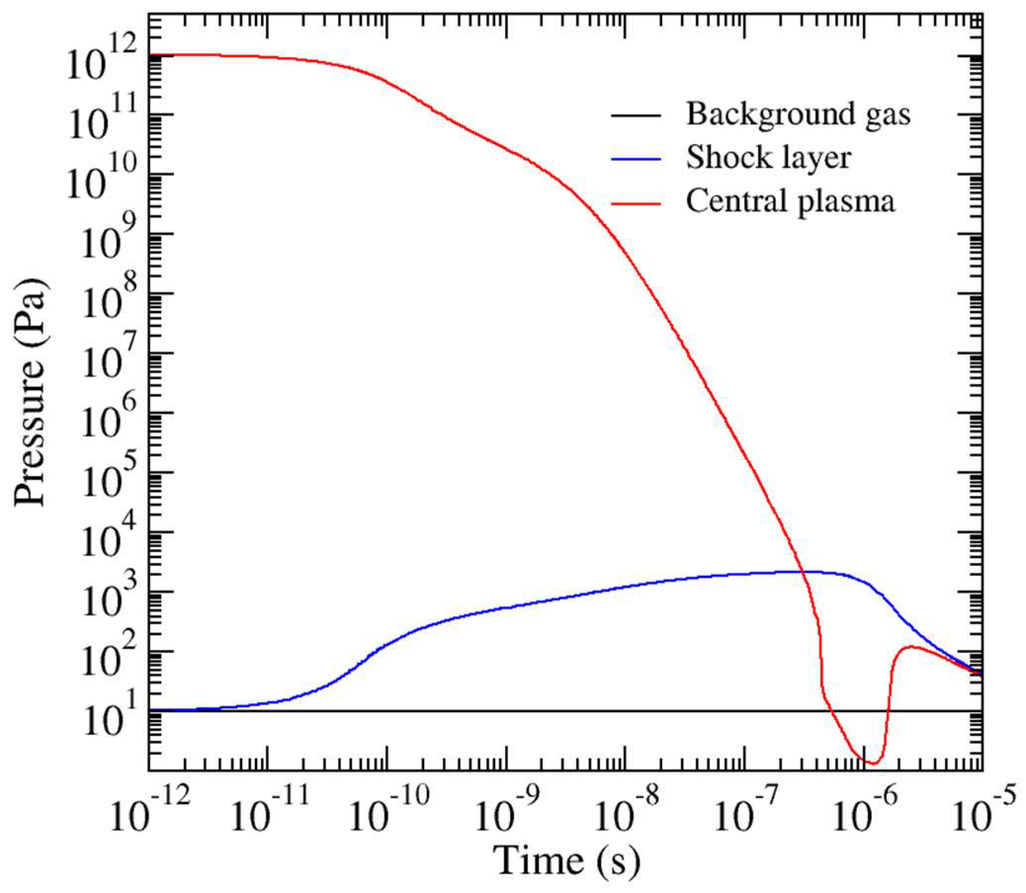
Figure 7 illustrates the pressure evolution in the central plasma and in the shock layer. Due to the initial pressure of the central tungsten plasma, the expansion starts around and induces the compression of the external background gas whose pressure increases in the shock layer. The expansion leads to the decrease in the pressure of the central plasma until sufficient inversion with respect to the shock layer. Then a recompression of the central plasma due to the shock layer takes place before a coupling between the two layers from the pressure point of view observed along the remaining part of the evolution.
In the framework of the present assumptions in terms of flow continuity, a minimum pressure of can be considered for argon. Figure 8 illustrates the pressure evolution of the layers in this case. We see that the recompression does not take place. The outside pressure is too low to ensure the confinement of the plasma. Its lifetime is therefore considerably shortened.
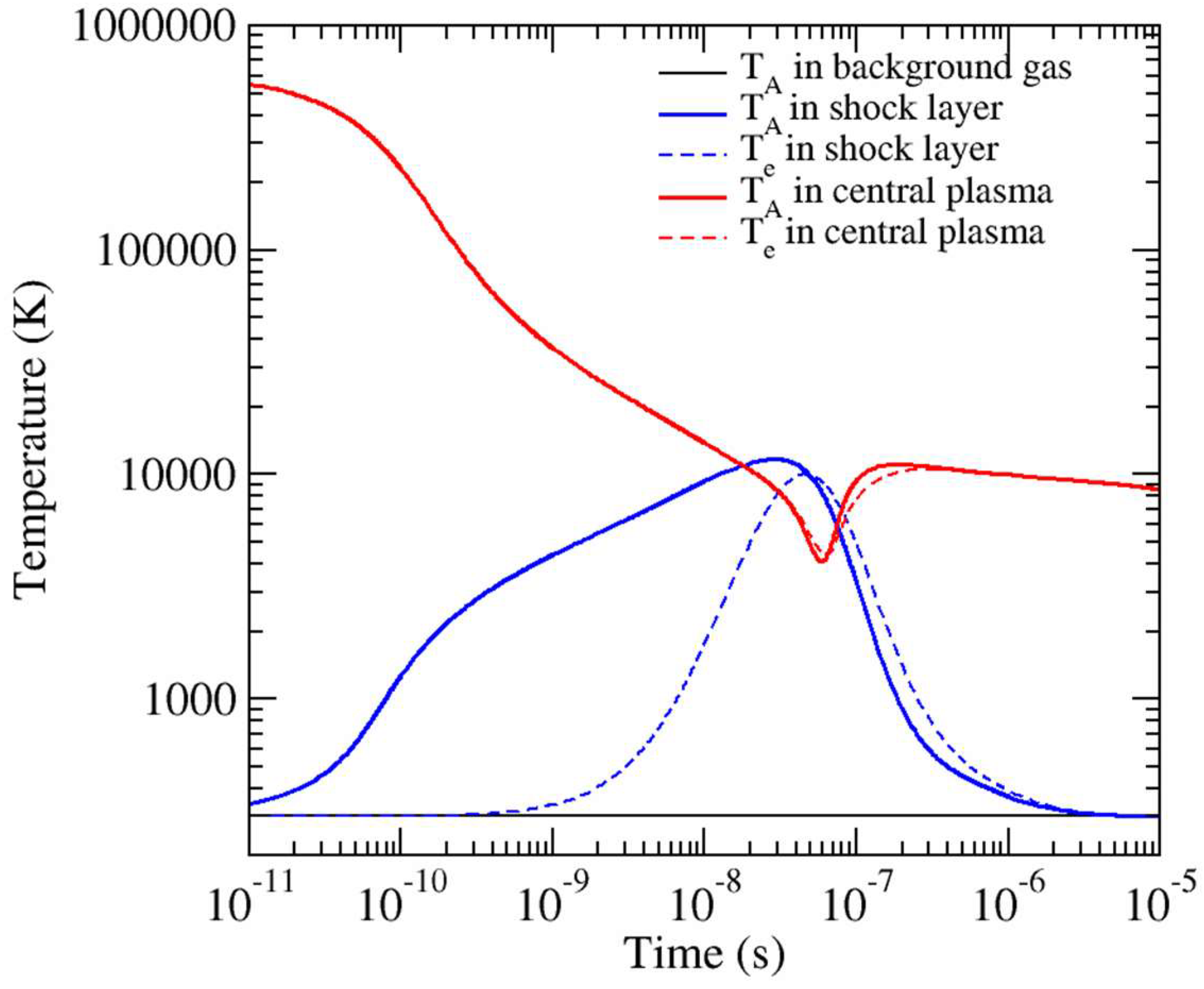
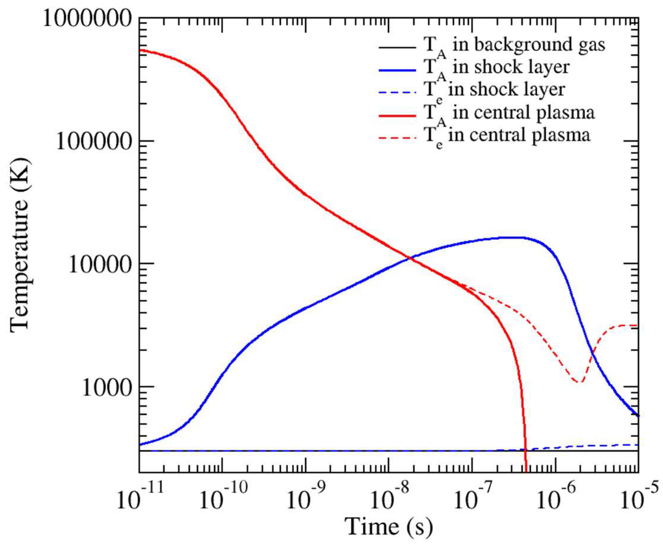
These trends can be also observed on the temperature evolutions of the different layers. Figure 9 illustrates the results for an argon gas at atmospheric pressure and Figure 10 those obtained at . It is interesting to see on Figure 9 that the thermal coupling resulting from the elastic collisions is efficient in the central plasma due to the high level of pressure. This is not the case for the shock layer where along almost the complete evolution. In the case of a pressure for the background gas, the thermal coupling is satisfactory in the central plasma until a characteristic time of the order of . Before this time, the evolution is quite the same as the one obtained at atmospheric pressure until . The plasma evolves independently from the presence of the background gas. Then, the pressure has sufficiently decreased, and the collision frequency is too weak to ensure the coupling between and . Electron density is very weak and the energy of the plasma is mainly stored in the kinetic energy due to expansion. Internal energy collapses: temperature rapidly decreases.
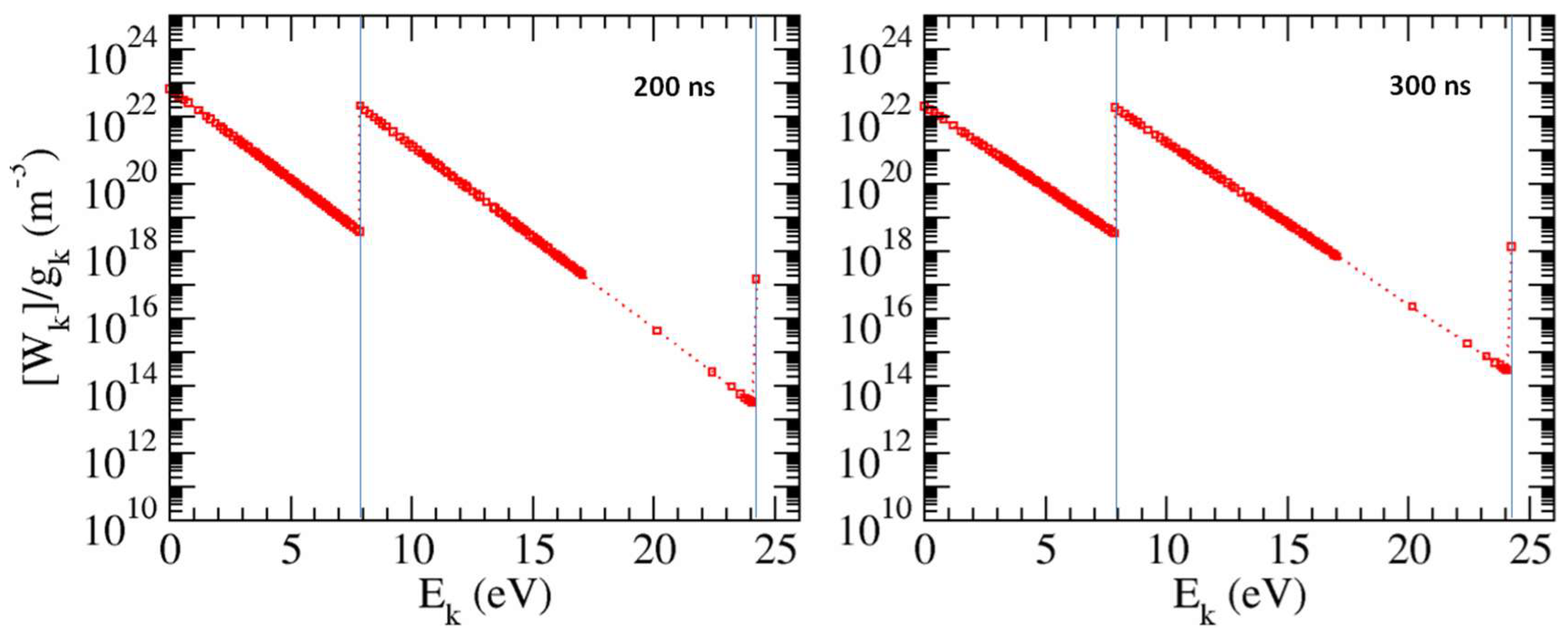
Our state-to-state approach enables the analysis of the departure from excitation equilibrium. Figure 11 displays the Boltzmann plots of the excited states of W and W+ in the central plasma at and at atmospheric pressure. Figure 12 displays those related to a argon gas.
On Figure 11, we clearly see that equilibrium is reached. The distribution is perfectly linear. We can also see that temperature is high since W2+ ions have a density of the order of , but temperature is too weak to influence the electron density . Indeed, we have . At , the situation is almost the same. A weak decrease in can be observed. This means that the collisional frequency is high enough to maintain in time the plasma situation.
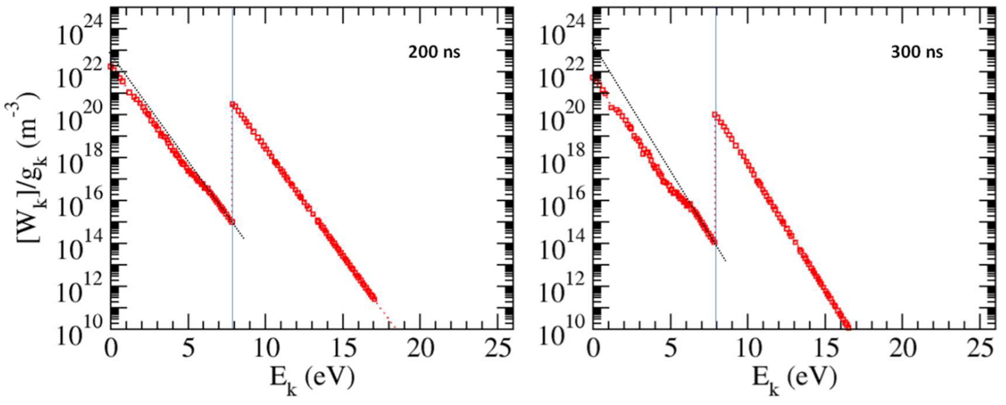
When the argon background gas pressure is decreased at , the situation is deeply modified. We can see that the main slope of the distribution of neutral or ionic excited states is more negative. The excitation temperature is therefore lower. Electron density is decreased with respect to the atmospheric pressure situation. Indeed, the electron density reaches at , and at . Moreover, we can see that the distribution departs from a linear behavior. The excited states just below the ionization limit on a interval are satisfactorily coupled according to a linear distribution, whereas the lower excited states have a fluctuating behavior increasing with time. We are, in the present case, in a strong recombination situation where the recombination induces a satisfactory coupling of the involved excited states at number density values higher than those expected due to the lower excited states. This very common behavior has been already observed in other situations. In an ionization situation similar to post-shock flows observed in atmospheric entries, the ionization induces the fast depopulating of the excited states of atoms close to the ionization limit, which leads to a depletion of these states in terms of density. Then, this is the exact symmetric case.
Over the whole energy diagram, the distribution cannot be linear. We have also to analyze the influence of radiation. At , the order of magnitude of the number density of the excited states close to is low. We have whereas for argon at atmospheric pressure. In these low density conditions, the influence of radiation is much more significant. Radiation causes departures from a linear distribution whose linearity cannot be recovered by the collisional coupling. At , the situation is worse since the collisional frequency is collapsing.
These behaviors have important consequences regarding the LIBS diagnostic. In case the LIBS experiments are performed at atmospheric pressure, the equilibrium is rapidly obtained. As a result, the estimate of the excited states population density and of the electron density is sufficient to derive the ground state number density. Using the same number of Boltzmann plots as the number of different species, the composition of the plasma, therefore of the sample, can be identified.
In the case when the experiments are performed at low pressure, the analysis is considerably more difficult. Indeed, it is not directly possible to derive the ground states number density from the analysis of the radiation produced during the deexcitation of the excited states. The distribution of the excited states departs from excitation equilibrium. Then, the development of collisional-radiative models based on state-to-state approaches is therefore mandatory, except if known samples are available whose composition similar to the one to be obtained have been previously determined. In that case, the composition will be directly derived from comparisons with these calibrated samples.
4. Conclusions
Our objective was to give the main information regarding the underlying physics involved by two examples of plasma flows departing from thermochemical equilibrium. The cases of the planetary atmospheric entry plasmas and of the laser-induced plasmas have been discussed.
Modeling strategies have been detailed for two particular situations. For the atmospheric entry plasmas, we have focused our attention on the Martian missions of the EXOMARS type. For the laser-induced plasmas, we have detailed the properties of the plasma flow produced during a LIBS experiment on a divertor tungsten tile. Since the excitation equilibrium condition is not fulfilled, the only relevant way is to develop a state-to-state description of the species, i.e., to consider each excited state of the species as an independent variable and to solve the conservation equations in this framework. This requires the elaboration of a collisional-radiative model taking into account the different elementary processes at the level of each state. This strategy needs enough numerical means since the number of excited species and of elementary processes is often prohibitive.
The results show that the excitation equilibrium can be observed if the collisional frequency is high enough to overcome the perturbative role of radiation. As a result, even in case of thermal non-equilibrium, the observed excitation equilibrium takes place at the translational temperature of the main collision partner.
Author Contributions
The authors have jointly contributed to the work described in this paper.
Funding
This work has been carried out within the framework of the ICOTOM project funded by the French Space Agency CNES (Centre National d’Etudes Spatiales). This work has been also carried out within the framework of the French Federation for Magnetic Fusion Studies (FR-FCM) and of the Eurofusion consortium, and has received funding from the Euratom research and training programme 2014–2018 and 2019–2020 under grant agreement no. 633053. This work has been also carried out within the framework of the TRANSAT project and has received funding from the Euratom Research and Training Programme 2014–2018 under grant agreement no. 754586. The views and opinions expressed herein do not necessarily reflect those of the European Commission. This work has been also funded by the French ANR (Agence Nationale de la Recherche) through the programme “Investissement d’Avenir” (ANR-10-LABX-09-01), LabEx EMC3, PICOLIBS project.
Conflicts of Interest
The authors declare no conflict of interest.
References
- Capitelli, M.; Armenise, I.; Bruno, D.; Cacciatore, M.; Celiberto, R.; Colonna, G.; De Pascale, O.; Diomede, P.; Esposito, F.; Gorse, C.; et al. Non-equilibrium plasma kinetics: A state-to-state approach. Plasma Sources Sci. Technol. 2007, 16, 830. [Google Scholar] [CrossRef]
- Capitelli, M.; Celiberto, R.; Colonna, G.; D’Ammando, G.; De Pascale, O.; Diomede, P.; Esposito, F.; Gorse, C.; Laricchiuta, A.; Longo, S.; et al. Plasma kinetics in molecular plasmas and modeling of reentry plasmas. Plasma Phys. Control. Fusion 2011, 53, 124007. [Google Scholar] [CrossRef]
- Anderson, J.D. Hypersonic and High Temperature Gas Dynamics; McGraw-Hill: New York, NY, USA, 1988; ISBN 9780070016729. [Google Scholar]
- Park, C. Nonequilibrium Hypersonic Aerothermodynamics; Wiley: New York, NY, USA, 1990; ISBN 978-0471510932. [Google Scholar]
- Cooke, R.D.; Engle, J.H. Entry flight testing the Space Shuttle, 1977 to 1984. In Proceedings of the AIAA Flight Testing Conference, AIAA AVIATION Forum, AIAA 2016-3357, Washington, DC, USA, 13–17 June 2016. [Google Scholar] [CrossRef]
- West, T.K.; Brandis, A.M. Updated stagnation point aeroheating correlations for Mars entry. In Proceedings of the 2018 Joint Thermophysics and Heat Transfer Conference, AIAA AVIATION Forum, AIAA 2018-3767, Atlanta, GE, USA, 25–29 June 2018. [Google Scholar] [CrossRef]
- Aboudan, A.; Colombatti, G.; Bettanini, C.; Ferri, F.; Lewis, S.; Van Hove, B.; Karatekin, O.; Debei, S. ExoMars 2016 Schiaparelli Module Trajectory and Atmospheric Profiles Reconstruction. Space Sci. Rev. 2018, 214, 97. [Google Scholar] [CrossRef]
- Gülhan, A.; Thiele, T.; Siebe, F.; Kronen, R. Combined Instrumentation Package COMARS+ for the ExoMars Schiaparelli Lander. Space Sci. Rev. 2018, 214, 12. [Google Scholar] [CrossRef]
- Le Brun, A.L.; Omaly, P. Investigation of radiative heat fluxes for Exomars entry in the Martian atmosphere. ESA Spec. Publ. 2011, 689, 22. [Google Scholar]
- Bultel, A.; Annaloro, J. Elaboration of collisional-radiative models for flows related to planetary entries into the Earth and Mars atmospheres. Plasma Sources Sci. Technol. 2013, 22, 025008. [Google Scholar] [CrossRef]
- Annaloro, J.; Bultel, A. Vibrational and electronic collisional-radiative model in air for Earth entry problems. Phys. Plasmas 2014, 21, 123512. [Google Scholar] [CrossRef]
- Bourdon, A.; Bultel, A. Numerical simulation of stagnation line nonequilibrium airflows for reentry applications. J. Thermophys. Heat Transf. 2008, 22, 168–177. [Google Scholar] [CrossRef]
- Miziolek, A.W.; Palleschi, V.; Schechter, I. Laser-Induced Breakdown Spectroscopy; Cambridge University Press: Cambridge, UK, 2006; ISBN B000SRGFR2. [Google Scholar]
- Morel, V.; Bultel, A.; Schneider, I.F.; Grisolia, C. State-to-state modeling of ultrashort laser-induced plasmas. Spectrochim. Acta Part B 2017, 127, 7–19. [Google Scholar] [CrossRef]
- Morel, V.; Pérès, B.; Bultel, A.; Hideur, A.; Grisolia, C. Picosecond LIBS diagnostics for Tokamak in situ plasma facing materials chemical analysis. Phys. Scr. 2016, T167, 014016. [Google Scholar] [CrossRef]
- NIST Database. Available online: https://dx.doi.org/10.18434/T4W30F (accessed on 24 September 2018).
- Morel, V.; Bultel, A.; Annaloro, J.; Chambrelan, C.; Edouard, G.; Grisolia, C. Dynamics of a femtosecond/picosecond laser-induced aluminum plasma out of thermodynamic equilibrium in a nitrogen background gas. Spectrochim. Acta Part B 2015, 103, 112–123. [Google Scholar] [CrossRef]
Figure 1.
Global situation close to the TPS of a spatial vehicle showing the structure of the shock layer, the motion of fluid particles and the boundary layer. is the typical thickness of the shock layer and the one of the boundary layer.
Figure 1.
Global situation close to the TPS of a spatial vehicle showing the structure of the shock layer, the motion of fluid particles and the boundary layer. is the typical thickness of the shock layer and the one of the boundary layer.

Figure 2.
Post-shock relaxation for the pressure, the mass density and the speed resulting from Equations (3)–(6). Since the diffusion phenomena are assumed negligible in these equations, the solution corresponds to the real flow before .
Figure 2.
Post-shock relaxation for the pressure, the mass density and the speed resulting from Equations (3)–(6). Since the diffusion phenomena are assumed negligible in these equations, the solution corresponds to the real flow before .

Figure 3.
Evolution with the position from the shock front (indicated on the right) of the Boltzmann plot of the CO2() vibrational states. The vibrational excitation energy relative to the ground state is given in abscissa. The dissociation energy of the CO2 molecule is reminded.
Figure 3.
Evolution with the position from the shock front (indicated on the right) of the Boltzmann plot of the CO2() vibrational states. The vibrational excitation energy relative to the ground state is given in abscissa. The dissociation energy of the CO2 molecule is reminded.

Figure 4.
Distribution of the number density of the different species taken into account in the chemistry (see Table 1) behind the shock front. Same as Figure 2: the solution is relevant with respect to the real situation until from the shock front.

Figure 5.
Distribution of the electron temperature , the heavy particle temperature , and the post-processed energy-dependent vibrational temperature of CO2 for the first (symmetric stretching) mode, second (bending) mode and third (asymmetric stretching) mode. The total energy-dependent vibrational temperature is also displayed. The limit of the boundary layer is located at : in the red region, feature of the flow in case of infinite shock layer thickness.

Figure 6.
Laser-induced plasma situation. The laser pulse is focused on the sample using a converging lens at an irradiance higher than the breakdown threshold. The ablated material expands according to a hypersonic regime and produces a shock wave propagating in the background gas. As a result, two layers are formed. The first one corresponds to the ablated material and the second one corresponds to the shock layer. These two layers are separated by a contact surface across which the diffusion phenomena can be considered as negligible in a first approximation.

Figure 7.
Evolution of the pressure inside the central tungsten plasma and inside the shock layer (case of argon) for a classical laser (, , )-induced plasma experiment at atmospheric pressure.
Figure 7.
Evolution of the pressure inside the central tungsten plasma and inside the shock layer (case of argon) for a classical laser (, , )-induced plasma experiment at atmospheric pressure.

Figure 8.
Same as Figure 7, but with an argon pressure of .
Figure 8.
Same as Figure 7, but with an argon pressure of .

Figure 9.
Same as Figure 7, but for the temperatures.
Figure 9.
Same as Figure 7, but for the temperatures.

Figure 10.
Same as Figure 8, but for the temperatures.
Figure 10.
Same as Figure 8, but for the temperatures.

Figure 11.
Boltzmann plots at and for an argon gas at atmospheric pressure. The first () and second ionization () limits are indicated by a vertical blue line. Each state is represented by a square. We see the added states following a hydrogen-like assumption between and .
Figure 11.
Boltzmann plots at and for an argon gas at atmospheric pressure. The first () and second ionization () limits are indicated by a vertical blue line. Each state is represented by a square. We see the added states following a hydrogen-like assumption between and .

Figure 12.
Same as Figure 11, but with an argon gas at . The second ionization limit is not displayed since the corresponding number densities are very weak. The line interpolating the excited states just below the first ionization limit is plotted to easily estimate the departure from excitation equilibrium.


Table 1.
List of the species and their excited states involved in CoRaM-MARS, the CR model developed at the CORIA laboratory for the CO2-N2-Ar mixtures.
Table 1.
List of the species and their excited states involved in CoRaM-MARS, the CR model developed at the CORIA laboratory for the CO2-N2-Ar mixtures.
| Species | States |
|---|---|
| CO2 | X1Σg+ (14 states (v1,v2,v3) with Ev < 0.8 eV, 106 states (i00,0j0,00k) with Ev > 0.8 eV), 3Σu+, 3Δu, 3Σu− |
| N2 | X1Σg+ (v = 0 → 67), A3Σu+, B3Πg, W3Δu, B’3Σu−, a’1Σu−, a1Πg, w1Δu, G3Δg, C3Πu, E3Σg+ |
| O2 | X3Σg− (v = 0 → 46), a1Δg, b1Σg+, c1Σu−, A’3Δu, A3Σu+, B3Σu−, f1Σu+ |
| C2 | X1Σg+ (v = 0 → 36), a3Πu, b3Σg−, A1Πu, c3Σu+, d3Πg, C1Πg, e3Πg, D1Σu+ |
| NO | X2Π (v = 0 → 53), a4Π, A2Σ+, B2Π, b4Σ−, C2Π, D2Σ+, B’2Δ, E2Σ+, F2Δ |
| CO | X1Σ+ (v = 0 → 76), a3Π, a’3Σ+, d3Δ, e3Σ−, A1Π, I1Σ−, D1Δ−, b3Σ+, B1Σ+ |
| CN | X2Σ+ (v = 0 → 41), A2Π, B2Σ+, D2Π, E2Σ+, F2Δ |
| N2+ | X2Σg+, A2Πu, B2Σu+, a4Σu+, D2Πg, C2Σu+ |
| O2+ | X2Πg, a4Πu, A2Πu, b4Σg− |
| C2+ | X4Σg−, 12Πu, 4Πu, 12Σg+, 22Πu, B4Σu−, 12Σu+ |
| NO+ | X1Σ+, a3Σ+, b3Π, W3Δ, b’3Σ−, A’1Σ+, W1Δ, A1Π |
| CO+ | X2Σ+, A2Π, B2Σ, C2Δ |
| CN+ | X1Σ+, a3Π, 1Δ, c1Σ+ |
| N | 4S°3/2, 2D°5/2, 2D°3/2, 2P°1/2, … (252 states) |
| O | 3P2, 3P1, 3P0, 1D2 … (127 states) |
| C | 3P0, 3P1, 3P2, 1D2 … (265 states) |
| Ar | 1S0, 2[3/2]°2, 2[3/2]°1, 2[1/2]°0, … (379 states) |
| N+ | 3P0, 3P1, 3P2, 1D2 … (9 states) |
| O+ | 4S°3/2, 2D°5/2, 2D°3/2, 2P°3/2, … (8 states) |
| C+ | 2P°1/2, 2P°3/2, 4P1/2, 4P3/2, … (8 states) |
| Ar+ | 2P°3/2, 2P°1/2, 2S1/2, 4D7/2, … (7 states) |
Table 2.
Jump conditions in due to the Rankine–Hugoniot assumption at altitude corresponding to the peak heating.
Table 2.
Jump conditions in due to the Rankine–Hugoniot assumption at altitude corresponding to the peak heating.
| Variable | Upstream Conditions | Conditions in |
|---|---|---|
| Speed () | 5270 | 690 |
| Mach number | 26.4 | 0.34 |
| Pressure () | 7.6 | 6000 |
| Temperature () | 162 | 16,800 |
Table 3.
List of the species and their excited states involved in the CR model CoRaM-Ar and CoRaM-W developed at the CORIA laboratory for the laser-induced plasmas on W in a rare gas (here for argon).
Table 3.
List of the species and their excited states involved in the CR model CoRaM-Ar and CoRaM-W developed at the CORIA laboratory for the laser-induced plasmas on W in a rare gas (here for argon).
| Plasma Layer | Species | States |
|---|---|---|
| (1) shock layer | Ar | 1S0, 2[3/2]°2, 2[3/2]°1, 2[1/2]°0, … (90 states) |
| Ar+ | 2P°3/2, 2P°1/2, 2S1/2, 4D7/2, … (7 states) | |
| Ar2+ | X2Σu+ | |
| (2) central plasma | W | 5D0, 5D1, 5D2, 5D3, … (60 states) |
| W+ | 6D1/2, 6D3/2, 6D5/2, 6D7/2, … (74 states) | |
| W2+ | 5D0…4, 3P20…2, 5F1…5, 3H4…6, 3F22…4 (5 states) |
© 2019 by the authors. Licensee MDPI, Basel, Switzerland. This article is an open access article distributed under the terms and conditions of the Creative Commons Attribution (CC BY) license (http://creativecommons.org/licenses/by/4.0/).
Share and Cite
MDPI and ACS Style
Bultel, A.; Morel, V.; Annaloro, J. Thermochemical Non-Equilibrium in Thermal Plasmas. Atoms 2019, 7, 5. https://doi.org/10.3390/atoms7010005
AMA Style
Bultel A, Morel V, Annaloro J. Thermochemical Non-Equilibrium in Thermal Plasmas. Atoms. 2019; 7(1):5. https://doi.org/10.3390/atoms7010005
Chicago/Turabian StyleBultel, Arnaud, Vincent Morel, and Julien Annaloro. 2019. "Thermochemical Non-Equilibrium in Thermal Plasmas" Atoms 7, no. 1: 5. https://doi.org/10.3390/atoms7010005
Note that from the first issue of 2016, this journal uses article numbers instead of page numbers. See further details here.