Selection of an Optimal Distribution Curve for Non-Stationary Flood Series
by
 , ,
, ,
Xiaohong Chen
1,2 ,
,
Changqing Ye
3,* ,
,
Jiaming Zhang
1,2,
Chongyu Xu
4,
Lijuan Zhang
1,2 and
Yihan Tang
1,2 1
Department of Water Resources and Environment, Sun Yat-sen University, Guangzhou 510275, China
2
Key Laboratory of Water Cycle and Water Security in Southern China of Guangdong High Education Institute, Sun Yat-sen University, Guangzhou 510275, China
3
Institute of Tropical Agriculture and Forestry, Hainan University, Haikou 570228, China
4
Department of Geosciences, University of Oslo, 0315 Oslo, Norway
*
Author to whom correspondence should be addressed.
Atmosphere 2019, 10(1), 31; https://doi.org/10.3390/atmos10010031
Submission received: 15 November 2018
/
Revised: 4 January 2019
/
Accepted: 10 January 2019
/
Published: 15 January 2019
(This article belongs to the Special Issue Flood Control and Management)
Abstract
:The stationarity assumption of hydrological processes has long been compromised by human disturbances in river basins. The traditional hydrological extreme-value analysis method, i.e., “extreme value theory” which assumes stationarity of the time series, needs to be amended in order to adapt to these changes. In this paper, taking the East River basin, south China as a case study, a framework was put forward for selection of a suitable distribution curve for non-stationary flood series by using the time-varying moments (TVM). Data used for this study are the annual maximum daily flow of 1954–2009 at the Longchuan, Heyuan and Boluo Stations in the study basin. Five types of distribution curves and eight kinds of trend models, for a combination of 40 models, were evaluated and compared. The results showed that the flood series and optimal distribution curves in the East River basin have been significantly impacted by a continuously changing environment. With the increase of the degree of human influence, the thinner tails of distributions are more suitable for fitting the observed flow data, and the trend models are changed from CP (mean and standard deviation fitted by parabolic trend model) to CL (mean and standard deviation fitted by linear trend model) from upstream to downstream of the catchment. The design flood flow corresponding to a return period of more than 10 years at the Longchuan, Heyuan and Boluo Stations was overestimated by more than 28.36%, 53.24% and 26.06%, respectively if the non-stationarity of series is not considered and the traditional method is still used for calculation. The study reveals that in a changing environment, more advanced statistical methods that explicitly account for the non-stationarity of extreme flood characteristics are required.
1. Introduction
Under the influences of climate change and human activities, significant changes are occuring to the hydrological regimes of many rivers, and the occurrence frequency of extreme hydrological events has also significantly increased [1]. Schiermeier (2011) pointed out that the rainfall intensity in the northern hemisphere showed an increasing trend in the late 20th century, leading to an increase in flood risk [2]. Barnett et al. (2008) found that in the second half of the 20th century, significant changes had occurred to the water cycle in the western USA, 60% of which were caused by human-induced environmental changes [3]. In the context of global warming, the frequency and intensity of extreme weather events in the past 50 years showed a strengthening trend in China, mainly reflected by the extent and frequency of floods and other extreme events [4].
It was pointed out by Milly et al. (2008) that stationarity is dead because substantial anthropogenic change of the Earth’s climate is altering the means and other statistics of precipitation, evapotranspiration, and rates of discharge of rivers [5]. Many hydraulic structures designed by the conventional hydrologic analysis methods, which have stationarity assumption, will face the distortion risk in design frequency caused by the ever-changing environment [6,7]. Compared with hydrologic frequency analysis method under the stationary assumption, which has a history of approximately 100 years, the flood frequency analysis of non-stationary hydrological series is an emerging research field, and recent research has continued to show a rapid development in this line [6,7,8,9,10].
The non-stationary flood frequency analysis methods mainly include several aspects, i.e., time-varying moments, pooled flood frequency analysis, local likelihood, quantile regression and mixture distribution model based on conditional probability [8,11]. Different methods of non-stationary flood frequency analysis were suggested for eliminating the trend in the time series through one or more processing steps [8]. One of the more general methods of non-stationary flood frequency analysis has been the streamflow naturalization methodology, but it needs to collect a lot of data [4]. With the deepening of research on the influences of environmental change on hydrologic processes, research on hydrologic frequency analysis under non-stationary conditions has been receiving special attention in recent years [12,13,14,15,16,17]. The method of time-varying moments (TVM) has become a commonly used method of non-stationary flood frequency analysis, because the TVM method can process the whole non-stationary flood series directly [18]. The time-varying parameters can be estimated with a combination of the analysis on trend, periodicity and other deterministic components [13]. It was found in the study of Diehl and Potter (1987) that the samples of extreme value series used for frequency analysis do not always originate from the same population, i.e., not subject to the same distribution, so that the mixture distribution model was proposed directly based on extreme sample series with non-identical distribution for frequency analysis [19]. In addition, some studies have aimed to establish a correlation between environmental factors and probability distribution parameters of hydrologic extreme value, and deduce the time-varying laws based on the variation laws of these factors [20,21].
A frequency analysis model of non-stationary extreme value series proposed by Strupczewski et al. (2001) embedded the trend component into the distribution of first and second-order moments (time-varying moments), i.e., the trends of mean and variance of statistical parameters were considered [12]. Recently, there have been many studies on TVM model. The study of Vogel et al. (2011) showed that the flood magnitude in many regions of the U.S. had an increasing trend, and floods with return periods of 100 years might become more common in some basins [22]. The generalized addictive model for Location, Scale and Shape parameters (GAMLSS) was used to study the flood peak flow series in the Little Sugar Creek Basin with a higher degree of urbanization by Villarini et al. (2009) [23]. It is shown that GAMLSS is able to describe the variability in the mean and variance of the annual maximum peak discharge by modeling the parameters of the selected parametric distribution as a smooth function of time via cubic splines.
Previous studies have shown that any violation of the basic hypotheses on independence and stationarity of observed data can significantly affect the accuracy of frequency analysis results [13,24,25]. However, there are few studies that focus on flood frequency distribution curve selection for non-stationary flood series. With the aim to understand the scientific and technical issues involved in the non-stationary flood frequency analyses, the non-stationary series processing methods with TVM were compared with the traditional frequency analysis method without non-stationary series processing, to analyze the flood frequency characteristics in the changing environment of the East River basin. By the end of 2005, many reservoirs of different sizes were gradually completed in the catchment area above the control station (Boluo Station) in the East River basin. The adjustment coefficient of the large reservoirs on runoff at the Boluo Station reached 0.34 step by step. Besides, the vegetation cover continuously keeps decreasing due to urbanization process in this area. Therefore, continuous human activities and climate changes have led to hydrological change in the East River basin [26,27,28,29,30]. The primary goal of this study was achieved through the following steps: (1) to reveal the mechanism of selecting the best fit distribution curves for non-stationary flood series from upstream to downstream that have been significantly affected by human activities and climate changes; and (2) to calculate and evaluate the impacts of the changing environment on the flood frequency distribution curve. Hydrological regimes in many basins in China and other developing countries are gradually changing due to climate change and human activities including the urbanization process and river regulations. The results of this study will be beneficial to rationally describe non-stationary extreme flood characteristics in the continuously changing environment of human-altered basins.
2. Study Area and Data
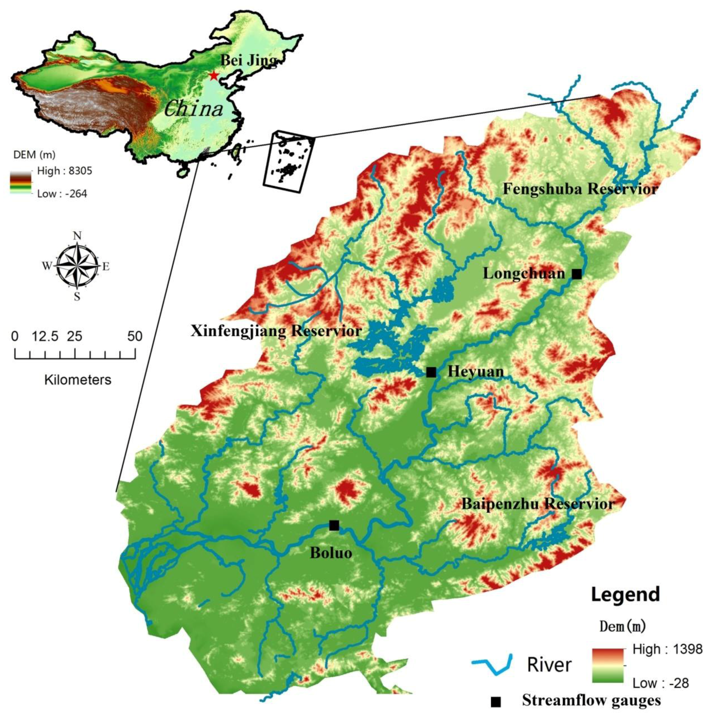
The East River basin is one of the main sub-basins in the Pearl River basin in south China (Figure 1), with a river length of 562 km and a total basin area of 27,040 km2. This basin belongs to a south subtropical monsoon climate zone. The water resources in the East River basin have been highly developed for urban water use, hydroelectric power generation and farmland irrigation, where the water use efficiency of the outer channel is more than 40%. The reservoirs in the East River basin control 51% of the entire basin area, and 12 cascade hydropower Stations have been constructed in the trunk channel [26]. The forest is the major land use type, whereas the urban area shows a rapid expansion, especially in the downstream areas [31].
The data used in the study include daily streamflow from three hydrological Stations for 1954–2009, i.e., Longchuan Station in the upper reach of East River basin, Heyuan Station in the middle reach, and Boluo Station in the lower reach, which were provided by the Hydrological Bureau of Guangdong Province. At present, three big reservoirs have been completed in the East River basin, i.e., Xinfengjiang, Fengshuba, and Baipenzhu, with a total storage capacity of 17.06 billion m3. The construction time of main reservoirs in the East River basin, the capacity of the reservoirs, the hydrological Stations affected by reservoirs and other information are shown in Table 1. In addition, there are thirty-six reservoirs above medium size and more than 661 small-sized reservoirs in the basin, which have been constructed continuously since 1950s to the present. The construction time of these hydraulic engineering structures spans the whole study period. Daily precipitation data for 1954–2009 were collected from 38 national standard rain gauges in the East River basin.
3. Methodology
In a changing environment, the flood return period estimated before the change is often unable to describe the flood frequency characteristics after environmental changes. This means that it is necessary to introduce a time reference point in describing the concept of return period.
Based on the concept of TVM, a method proposed by Strupczewski et al. (2001) to calculate the non-stationary flood frequency is used in this study [12]. This method considers the trend components of first and second order moments (mean m and standard deviation σ) of a probability distribution function. For the sake of completeness, the procedure of the method is briefly introduced in this section, and more detailed information of TVM method can refer to Strupczewski et al. (2001) and Yan et al. (2017a) [12,32].
3.1. Probability Distribution
The most commonly used frequency-magnitude distributions in hydrology can be divided into five groups: the normal family (normal, log-normal, log-normal type 3), the Generalized extreme-value (GEV) family (GEV, Gumbel, log-Gumbel, Weibull), the Pearson type 3 family (Pearson type 3, log-Pearson type 3), the generalized Pareto distribution and the general generalized logistic family (GLO) [33,34,35]. Five commonly used probability distributions were selected in this study including Pearson-III distribution (P3), Gumbel distribution (GMB), lognormal distribution (LN2), generalized extreme value distribution (GEV) and generalized logistic distribution (GLO), which represent the normal family, extreme-value family, Pearson type 3 family and general generalized logistic family (Table 2) [34,36].
For the three-parameter P3 distribution, the lower bound parameter in the distribution was considered to remain unchanged over time in this study [22,32,37]. GEV and GLO are also three-parameter distributions, however, these methods only consider the trend components of first two moments, i.e., among three parameters of the distributions, one parameter must not change over time [6,22]. The coefficient of skewness Cs is used to describe the shape of a distribution. Cs represents the extent of symmetry of a random variable with respect to the mean value. The middle part of frequency distribution shifts to the left as Cs increases with a steeper large flood part on the left and a flatter small flood part on the right. Parameter k is the shape parameter of GLO and GEV distributions, and has a certain correlation with Cs. Among GEV and GLO distributions, no lower bound parameters of random variable x exist, and the lower bound of x is determined by three parameters, while values of Cs and k have a fixed function relationship [38], i.e., Cs = Cs(k). Therefore, the shape parameter k correlated to Cs in GEV and GLO was considered to remain unchanged over time in this study.
3.2. Trend Model
In order to ensure the independence of the hydrological sequence, “extreme” refers to the annual maximum daily flow in this study, and only one sample is taken in a year. Data series used for this study are the annual maximum daily flow of 1954–2009 at the Longchuan, Heyuan and Boluo Stations. Due to the limited length of the data series, only the trends of first two moments were considered in this study with respect to the following situations:
1. Trend in mean values—(A);
2. Trend in standard deviations—(B);
3. Both the mean value and standard deviation have a trend and the ratio of the two (i.e., Cv) is constant—(C);
4. Both the mean value and standard deviation have a trend and the ratio of the two (i.e., Cv) is not constant—(D).
There is also a basic situation that neither of the first two moments has a trend, i.e., the distribution parameters do not change over time as a stationary option (S).
Among A, B, and C trend types, two further options exist: linear trend (L) or parabolic type (P).
For Type D, only linear trend was considered (L) in this study with the purpose of keeping the number of parameters to a minimum.
3.3. Parameter Estimation
3.4. Selection of Optimal Model
AIC (Akaike Information Criterion) not only rewards goodness of fit, but also includes a penalty, which is an increasing function of the number of estimated parameters. The AIC provides a means of model selection and evaluation based on the principle of maximum entropy [18]. In this study, the AIC is used as a criterion of goodness of fit. The calculation equation is shown as below:
where, ML is the maximum likelihood function, and k is the number of model parameters [39]. The model with the minimum AIC value should be selected as the optimum model.
4. Results
4.1. Non-Stationarity Detection in Flood Series
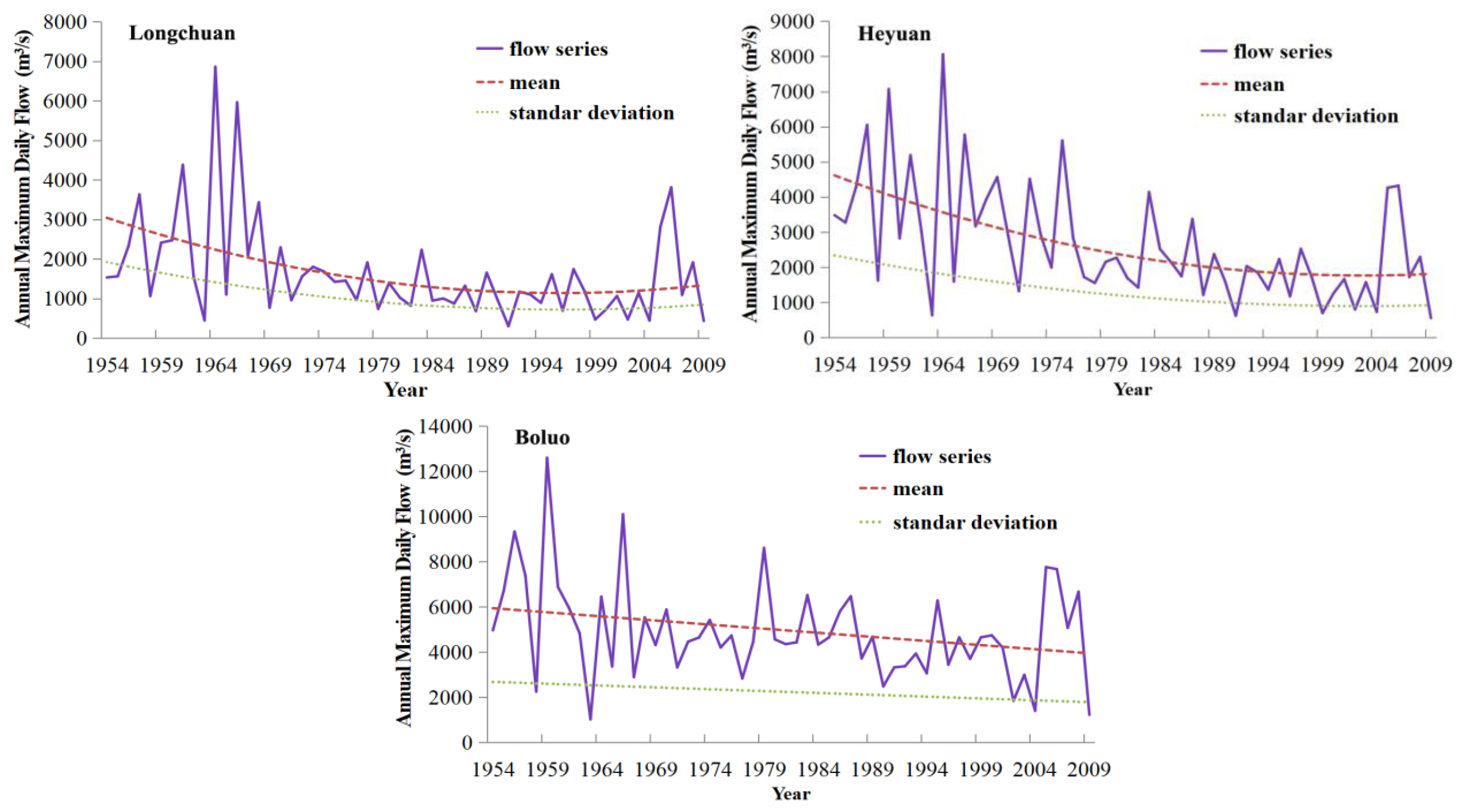
The changing trends of annual maximum peak flow of the three stations are detected by Mann-Kendall (M-K) test (Table 4) [40]. It is seen that a decreasing trend at the significance level of 0.05 or less (p < 0.05) exists in all three stations. Figure 2 is a visual illusion for describing the changing details, which shows that deluge events frequently occurred for the first two decades. Afterwards, the flood series of Longchuan Station showed a significant downward trend until 2004, and high flood events occurred between 2005 and 2007. The flood peak flows of Heyuan and Boluo Stations show a similar but relatively gentle changing pattern. Specifically, the annual maximum flood flow had a significant downward trend from 1954 to 2009. During the same period, the precipitation amounts in the Longchuan and Heyuan Stations have displayed a slightly decreasing tendency (Table 4). In contrast, the precipitation in the Boluo Station displayed a slightly increasing tendency, indicating that in addition to precipitation, other factors also affect flood changes. To better understand the possible factors for the flow change, we also collected the Normalized Difference Vegetation Index (NDVI). NDVI reflects the overall information for the ground vegetation. The data are from Global Inventory Modeling and Mapping Studies (GIMMS) [41]. It can be seen from Table 4 that the vegetation cover keeps decreasing due to the rapid urbanization that occurred in this area [26]. The percentage of urban area was 1.94 in 1990 and this increased to 4.79 in 2010, indicating rapid urban expansion during the interim years [31]. The rapid urbanization in the River basin can significantly increase the flood peak, causing more quick flow and therefore strengthening flood events, etc. (e.g., Zhang et al. 2015) [17]. This is contrary to the trend of the flood sequence. Therefore, the non-stationarity of hydrological series is impacted by continuous changing environment of multi-factor synthesis. The number of reservoirs and the water storage capacity are increasing gradually. The area of urban construction land is continuously expanding, and the change of climatic factors, especially the trend of rainfall, is also a slow process.
4.2. Selection of Optimal TVM Model
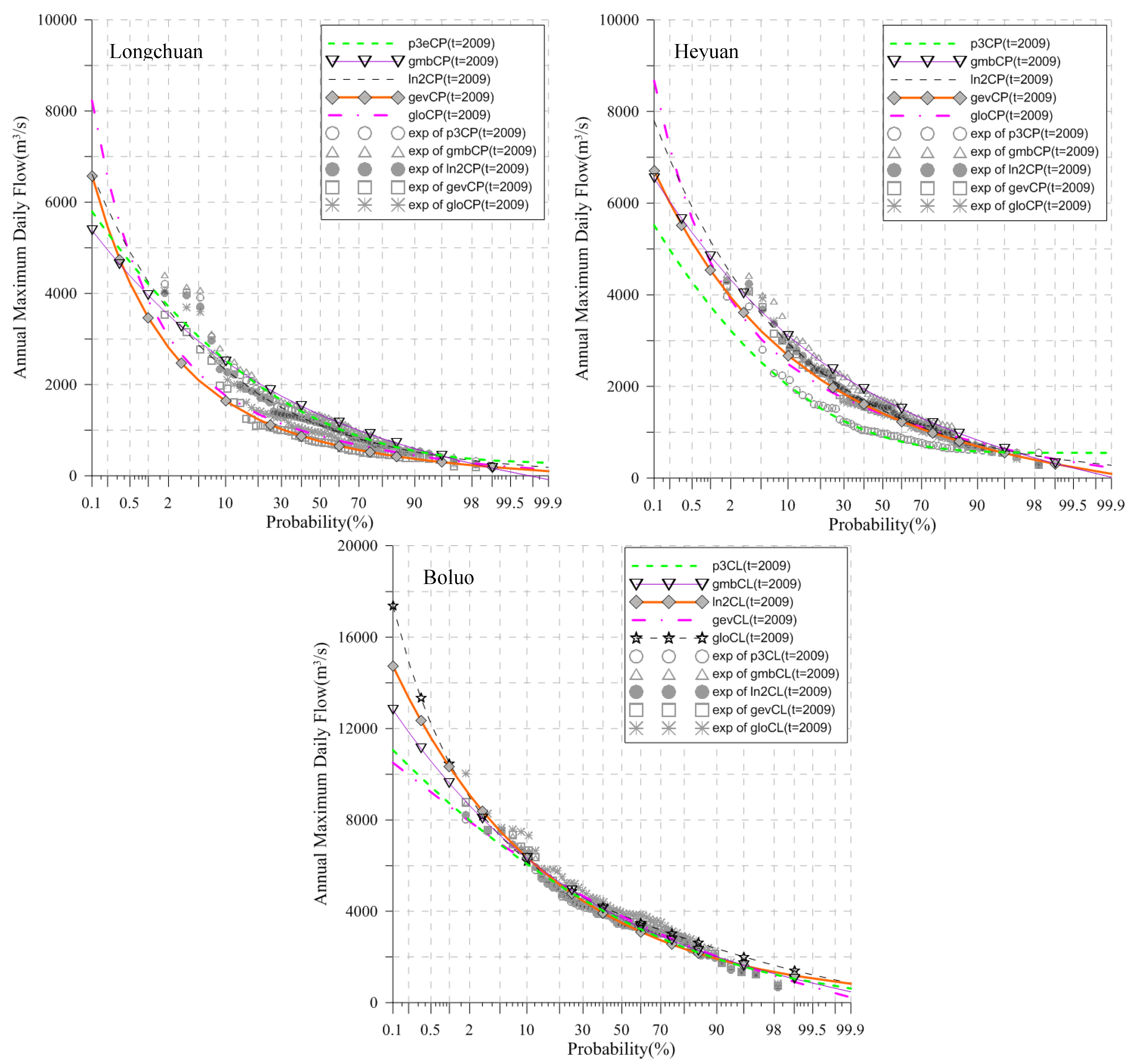
AIC was taken as the discrimination criterion of the optimal model (Table 5). Table 6 shows the parameter estimations for all distributions by MLE. It is seen from Table 5 that the LN2CP model at Longchuan, GMBCP model at Heyuan, and GMBCL model at Boluo Station were the best fitting models in terms of the AIC values. The performance of the optimal model selection using AIC can be analyzed from two aspects, i.e., from the characteristic of distribution curves and from the trend model, as detailed in the following sub-sections.
4.2.1. Selection of Optimal Distribution
The flood frequency curves of different distributions mainly show differences at the tails of the distribution, especially in the high flow part which generally shows big differences for different distributions. The values of coefficient of variation Cv and coefficient of skewness Cs for annual maximum flood peak flow data, gradually decreased from upstream to downstream of the catchment (Longchuan Cv = 0.775, Cs = 2.261; Heyuan Cv = 0.627, Cs = 1.211; Boluo Cv = 0.445, Cs = 1.008). In general, Cv and Cs are the important parameters for most distributions and different values of which will have significant influence on the design values. When Cv and Cs values are larger, the upper tail of frequency curve of flood series will change from “gentle” to “steep”, and the heavy tailed distribution is more flexible on this part and is more suitable for fitting the data. As can be seen from the study of Adlouni et al. (2008) [42], the tail of lognormal distribution is thicker than Gumbel distribution. This conclusion coincides with the result of our model selection, which shows that LN2 distribution is suitable for Longchuan Station in upstream, and Gumbel distribution is suitable for middle and lower reach Stations of Heyuan and Boluo (Figure 3) (Table 5).
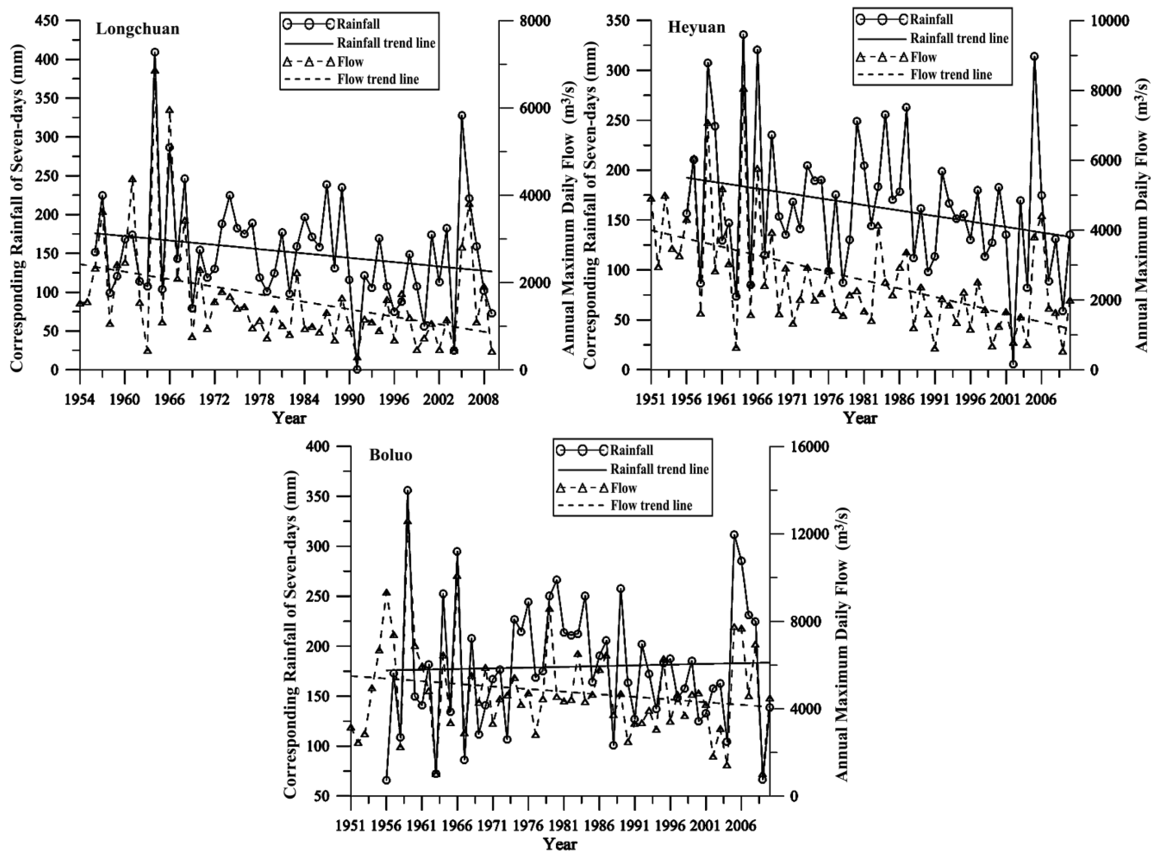
It would be important to understand the possible reasons for selecting different distributions. As rainfall is the primary source of streamflow in the study basin, the possible relationship between annual maximum streamflow and corresponding basin rainfall in the past 7 days was investigated. For Longchuan and Heyuan Stations, the flood series and the corresponding rainfall series are consistent with decreasing trend for both series, and for flood series the trend is statistically significant at the 0.05 level (Table 4), while the decreasing trend for the rainfall series is not significant at the 0.05 level (Figure 4). For Boluo Station, the flood series and the corresponding rainfall series are inconsistent with an increasing trend for rainfall series but a slightly decreasing trend for the flood series (Figure 4), meaning that the effect of rainfall on the flood is weakening. As a possible consequence, the Cs values of the peak flood series exhibit a decreasing trend from upstream to downstream, which may be caused by the variation of rainfall, urbanization activities and basin reservoir regulation storage. Due to the enhancing degree of human influence from upstream to downstream, the sensitivity of the stream flow to climate fluctuation gradually reduces from upstream to downstream in East River basin.
4.2.2. Selection of Optimal Trend Model
According to the trend model parameters of the optimal model (LN2CP for Longchuan, GMBCP for Heyuan, GMBCL for Boluo Station) (Figure 3) (Table 6), the change processes in means and standard deviations of flood series as showed in Figure 2 are discussed in the following paragraphs.
(1) The CP trend model for Longchuan station in the upper reaches. Referring to the seven different types of trend forms assumed in Section 3.2, in either A, B or C-type trend models, model parameters are ultimately obtained by fitting the observed series. Therefore, the potential trends of the mean and standard deviation are firstly determined by observed series intuitively. The means of observed flood flow series generally show a parabolic change trend as “decline–steady–rise” (Figure 2). Under the control of the CP model, the mean curve conforms to the change process of observed flood flow (Figure 2). It is necessary to consider the change trend of standard deviation for the hydrological extremes analysis. Standard deviation reflects the concentration degree of random variables. The smaller the standard deviation is, the more concentrated the random variables will be, while in contrast, the more easily the random variables will deviate from the average value, leading to an increase in the occurrence of extreme events. It was found that the flood peak values on both ends of the series were less concentrated; the entire series showed more intense flood peak changes in the first 20 years of the series with larger standard deviation. After 1976, the series has smaller standard deviation until 2004, followed by an increasing trend with standard deviation. In general, the change trends of the standard deviation and the mean are the same, i.e., a parabolic change trend of “decline-steady-rise”. The standard deviation curve of CP model is consistent with the standard deviation of the observed annual maximum peak flow (Figure 2). As a result, the CP trend model (mean and standard deviation related by the parabolic trend model) had a better fitting effect than other trend models.
(2) The CP trend model for Heyuan Station in the middle reaches. The flood peak flows of Heyuan Station show a similar changing pattern to Longchuan Station (Figure 2). As a result, the CP trend model had a better fitting effect than other trend models (Figure 2).
(3) The CL trend model for Boluo station in the lower reaches. The observed flood flow series exhibited linear decreasing trend (Figure 2). Under the control of the CL model, the mean curve conforms to the change process of observed flood flow. From the analysis of the change in standard deviation, it can be found that both the maximum and minimum flood peaks of the entire series occurred in the first 10 years of the series. However, the series after 1974 had smaller change amplitudes, fluctuated within a relatively concentrated range. In general, the standard deviation in the past 56 years had also experienced a process from large to small. The standard deviation curve of the CL model is consistent with standard deviation of the observed flood flow (Figure 2). Such change trends also existed in the mean, so that the CL model (mean and standard deviation related by the linear trend model) had a better fitting effect (Table 5).
It can be seen from the above results that after non-stationarity occurred to the flood series, all distribution parameters in terms of flood peak flows at three hydrological stations along the East River have changed (Figure 2). Combined with visual estimation, it was found that these trend curves of means and standard deviations were consistent with the change trends of flood peak series. In terms of distribution curves, the optimal distributions of non-stationary flood series in the East River basin were all mixed tail distributions. Therefore, the LN2CP parabolic curve at the Longchuan Station, the GMBCP parabolic curve at the Heyuan Station and the GMBCL linear model at the Boluo Station were selected for the optimal model (Figure 3).
4.3. Comparison of Return Period Obtained from TVM Model and Traditional Methods
The large-scale multiple reservoirs in the river basin can significantly reduce the flood volume and flood peak, change the rate of convergence of floods, and the time of the peak. Several studies (e.g., Zhang et al. 2015; Miller et al. 2013; Wei et al. 2017; Michelle et al. 2017) suggest that both the occurrence of extreme events and common floods of the rivers have decreased significantly, partly due to reduction effect of reservoirs [16,17,43,44]. In order to compare the differences in flood return period between non-stationary processing and traditional flood methods (traditional method is a frequency analysis method in which the hydrological sequence satisfies the stationarity assumption), relative difference degree E was used to quantitatively express the difference degree between the two. The equation is shown as below:
where, indicates the design flood flow of optimal curve with TVM model, and indicates the design flood flow with traditional methods.
Comparing the traditional curve LN2 with the TVM model at Longchuan Station, the difference of 10-year flood flows was 28.36%, while the difference of 100-year flood flows increased to 38.65% (Table 7). From another perspective, for the same flood flow, the return period obtained by the non-stationary processing approach is longer than that of the traditional methods. This is mainly because the flood peak reduction effect of Fengshuba Reservoir led to the non-stationary flood peak flow in Longchuan Station.
For the traditional curve GMB at Heyuan Station, the difference of design flood flows from TVM model and traditional methods corresponding to return periods of 10 years was 53.24%, and that with a flood peak corresponding to return periods of 100 years increased to 57.39% (Table 7). For the traditional curve GMB at Boluo Station, the difference of 10-year flood flows was 26.06%, and that of 100-year flood flows increased to 26.92% (Table 7).
5. Discussion
Correct selection of trend models for mean and standard deviation has a great impact on the estimated flow return period [10,17,18]. Even for the same distribution curve, the selection of different trend models will cause significant differences in the calculated return period. For example, GMBBL with poorer fitting effects at the Boluo Station was non-consistent with the standard deviation for observed series that changes from large to small in the period of 50 years. The return period was significantly reduced over time, opposite with the results of the optimal model that considers the non-stationarity. Therefore, in the calculation of non-stationary flood frequency, it is required not only to consider the change trend of the mean value of flood peak, but also to consider the change trend of standard deviation. AIC and other auto-selection criteria all have deficiencies, because most of the data information is covered in the overall statistics [39]. In the initial selection of the contrast model for time series, the intuitive judgments on the fitting degree and the length of time series must be considered. The first step should be to intuitively determine the potential trends of mean and standard deviation in the existing time series. The above phenomena reflect the fact that the parameter change of non-stationary flood series will cause a greater impact on the estimation of flood return period. The correct selection of change trend model for the parameters has a significant impact on flood design discharge, which should be considered in the engineering and hydrologic design.
The results of previous studies show that a changing environment in the river basins can significantly alter the flood volume and flood peak, and change the time of the peak. The impact of urbanization activities and the reservoirs on estimates of flood frequency is considerable [16,17,44]. Influenced by climate change and the degree of human activities, the tail-end of the high-water frequency curve declined significantly. The occurrence probability of the same magnitude of flood was significantly reduced, as was the real design flood magnitude. Both precipitation and runoff changed smoothly during the period, and the slight difference in the changing trend of runoff is caused by factors other than precipitation. One of the most important signs of human activity is land use change. Benefitting from the significant growth of population and Gross Domestic Product (GDP), technological progress and policy support, the downstream areas such as Shenzhen and Dongguan have accelerated the pace of urbanization since 1990s [45]. The percentage of urban area was 1.94 in 1990 and increased to 4.79 in 2010. The urban area downstream expanded most rapidly mainly by encroaching into the rice field, agricultural area, and forest land [31]. In addition, many reservoirs of different sizes have been constructed continuously from the 1950s to the present. The adjustment coefficient of the large reservoirs on runoff at the Boluo Station reached 0.34 [26]. The impact of reservoirs is similar to that of urbanization. They are not built in a short period of time, but are gradually built over the years of the whole study period.
The change factors that cause the “non-stationarity” of the flood series can be divided into two categories, i.e., continuous (e.g., urbanization, landuse change) factors and one-time (e.g., dam construction) factors. The TVM method is better suited for application on the condition of continuous change. For a situation of one-time change, TVM is of course not necessary, as we can split data into two stationary periods, i.e., pre- and post-construction periods, and fit different distributions separately. Climate change and landuse change can largely be regarded as continuous changes in the East River Basin. Multiple hydraulic engineering structures including reservoirs and locks which have been constructed year by year from the 1950s to the present in the study area also cause a continuous change tendency of flow series with some notable fluctuation. Therefore, the changed environment in the East River Basin can largely be regarded as the result of continuous changes with some notable influence of reservoir operations. If we would discuss only the impact of a single reservoir in a basin, it could not be considered as a continuous time series but instead as a one-time change time series, and it therefore would not be proper to use the TVM method. In a future study, it would be interesting to compare the influence of one-time factors vs. continuous factors on the goodness of fitting (e.g., dam volume vs. flow rate, urbanization vs. flow rate) in the East River basin or other basins influenced by multiple factors.
6. Conclusions
The flood series in the East River basin show non-stationarity in time impacted by continuous changing environment of multi-factor synthesis. In this study, the non-stationary processing method of time-varying moments was adopted to analyze and calculate the annual maximum daily flow series at the Longchuan, Heyuan and Boluo Stations of the East River basin. Five types of distribution curves and eight kinds of trend models, for a total of 40 models (including the case of no consideration on trend), were selected for comparison. We found that the non-stationarity of series has a significant influence on the results of frequency analysis, and this influence is station dependent, as the human activities have shown different impacts on different stations. The study has resulted in the following specific conclusions.
1. LN2 distribution with a CP model at Longchuan Station, GMB distribution with a CP model at Heyuan Station, and GMB distribution with a CL trend model at Boluo Station obtain the optimal fitting.
2. The flood series and optimal distribution curves selection in the East River basin have been significantly affected by the continuous changing environment. With the precipitation change, the continuous process of urbanization and the reservoirs storage-capacity increases, the thinner tails of distribution are more suitable for fitting the observed flow data, and the trend model is changed from CP to CL from upstream to downstream of the watershed.
3. If the non-stationarity of flood series is not considered and the traditional method is still used for calculation, the design flood magnitudes will be overestimated for all three stations. The design flood flows with a return period of more than 10 years at the Longchuan, Heyuan and Boluo Stations were overestimated by more than 28.36%, 53.24%, and 26.06%, respectively, and the overestimation will be enlarged with an increase in return period.
4. Compared with non-stationary flood series characteristics, the flood magnitude was smaller and the frequency was lower for the stationary “real” flood series characteristics after hydraulic engineering regulations were implemented.
Author Contributions
Conceptualization, X.C. and C.Y.; methodology, J.Z.; software, Y.T.; validation, C.Y., J.Z. and L.Z.; formal analysis, C.Y.; investigation, C.Y.; resources, X.C.; data curation, J.Z.; writing—original draft preparation, C.Y.; writing—review and editing, C.X.; visualization, L.Z.; supervision, X.C.; project administration, X.C.; funding acquisition, X.C.
Funding
The research is financially supported by the National Natural Science Foundation of China (Grant No. 51569009, 91547202, 51479216, 51509127), the National Science and Technology Support Program (Grant No 2012BAC21B0103), the project for Creative Research from Guangdong Water Resources Department (Grant No. 2011-11), Hainan Natural Science Foundation (414192,20164157), Young Scientists Academic Innovation Project of Hainan Association for Science and Technology (HAST201629), and the Research Council of Norway (FRINATEK Project 274310).
Acknowledgment
A collaborative contribution by the CSIRO Computation and Simulation Sciences Transformational Capability Platform is acknowledged.
Conflicts of Interest
The authors declare no conflict of interest.
References
- Liu, J.; Wang, S.-Y.; Li, D.-M. The analysis of the impact of land-use changes on flood exposure of wuhan in yangtze river basin, China. Water Resour. Manag. 2014, 28, 2507–2522. [Google Scholar] [CrossRef]
- Schiermeier, Q. Increased flood risk linked to global warming. Nature 2011, 470, 315. [Google Scholar] [CrossRef] [PubMed]
- Barnett, T.P.; Pierce, D.W.; Hidalgo, H.G.; Bonfils, C.; Santer, B.D.; Das, T.; Bala, G.; Wood, A.W.; Nozawa, T.; Mirin, A.A.; et al. Human-induced changes in the hydrology of the western united states. Science 2008, 319, 1080–1083. [Google Scholar] [CrossRef] [PubMed]
- Chen, X.; Tu, X.; Xie, P.; Li, Y. Progresses in the research of human induced variability of hydrological elements. Adv. Earth Sci. 2010, 25, 800–811. [Google Scholar]
- Milly, P.C.D.; Betancourt, J.; Falkenmark, M.; Hirsch, R.M.; Kundzewicz, Z.W.; Lettenmaier, D.P.; Stouffer, R.J. Climate change. Stationarity is dead: Whither water management? Science 2008, 319, 573–574. [Google Scholar] [CrossRef] [PubMed]
- Xiong, L.; Du, T.; Xu, C.-Y.; Guo, S.; Jiang, C.; Gippel, C.J. Non-stationary annual maximum flood frequency analysis using the norming constants method to consider non-stationarity in the annual daily flow series. Water Resour. Manag. 2015, 29, 3615–3633. [Google Scholar] [CrossRef]
- Hassanzadeh, Y.; Abdi, A.; Talatahari, S.; Singh, V.P. Meta-heuristic algorithms for hydrologic frequency analysis. Water Resour. Manag. 2011, 25, 1855–1879. [Google Scholar] [CrossRef]
- Khaliq, M.N.; Ouarda, T.B.M.J.; Ondo, J.C.; Gachon, P.; Bobée, B. Frequency analysis of a sequence of dependent and/or non-stationary hydro-meteorological observations: A review. J. Hydrol. 2006, 329, 534–552. [Google Scholar] [CrossRef]
- De Paola, F.; Giugni, M.; Pugliese, F. A harmony-based calibration tool for urban drainage systems. Proc. Instit. Civ. Eng.-Water Manag. 2018, 171, 30–41. [Google Scholar] [CrossRef]
- Hounkpè, J.; Diekkrüger, B.; Badou, D.; Afouda, A. Non-stationary flood frequency analysis in the ouémé river basin, benin republic. Hydrology 2015, 2, 210–229. [Google Scholar] [CrossRef]
- Singh, V.P.; Wang, S.X.; Zhang, L. Frequency analysis of nonidentically distributed hydrologic flood data. J. Hydrol. 2005, 307, 175–195. [Google Scholar] [CrossRef]
- Strupczewski, W.G.; Singh, V.P.; Feluch, W. Non-stationary approach to at-site flood frequency modelling i. Maximum likelihood estimation. J. Hydrol. 2001, 248, 123–142. [Google Scholar] [CrossRef]
- Cunderlik, J.M.; Burn, D.H. Non-stationary pooled frequency analysis. J. Hydrol. 2003, 276, 210–223. [Google Scholar] [CrossRef]
- Eum, H.-I.; Vasan, A.; Simonovic, S.P. Integrated reservoir management system for flood risk assessment under climate change. Water Resour. Manag. 2012, 26, 3785–3802. [Google Scholar] [CrossRef]
- Zeng, H.; Feng, P.; Li, X. Reservoir flood routing considering the non-stationarity of flood series in north China. Water Resour. Manag. 2014, 28, 4273–4287. [Google Scholar] [CrossRef]
- Wei, Q.; Sun, C.; Wu, G.; Pan, L. Haihe river discharge to bohai bay, north China: Trends, climate, and human activities. Hydrol. Res. 2017, 48, 1058–1070. [Google Scholar] [CrossRef]
- Zhang, Q.; Gu, X.; Singh, V.P.; Xiao, M.; Chen, X. Evaluation of flood frequency under non-stationarity resulting from climate indices and reservoir indices in the east river basin, China. J. Hydrol. 2015, 527, 565–575. [Google Scholar] [CrossRef]
- Chen, P.-C.; Wang, Y.-H.; You, G.J.-Y.; Wei, C.-C. Comparison of methods for non-stationary hydrologic frequency analysis: Case study using annual maximum daily precipitation in taiwan. J. Hydrol. 2017, 545, 197–211. [Google Scholar] [CrossRef]
- Diehl, T.; Potter, K.W. Mixed flood distributions in wisconsin. In Hydrologic Frequency Modeling; Singh, V.P., Ed.; D. Reidel Publishing Company: Dordrecht, The Netherlands, 1987; pp. 213–226. [Google Scholar]
- Katz, R.W.; Parlange, M.B.; Naveau, P. Statistics of extremes in hydrology. Adv. Water Resour. 2002, 25, 1287–1304. [Google Scholar] [CrossRef] [Green Version]
- Xiong, L.; Jiang, C.; Du, T. Statistical attribution analysis of the nonstationarity of the annual runoff series of the weihe river. Water Sci. Technol. 2014, 70, 939–946. [Google Scholar] [CrossRef]
- Vogel, R.M.; Yaindl, C.; Walter, M. Nonstationarity: Flood magnification and recurrence reduction factors in the united states. J. Am. Water Resour. Assoc. 2011, 47, 464–474. [Google Scholar] [CrossRef]
- Villarini, G.; Smith, J.A.; Serinaldi, F.; Bales, J.; Bates, P.D.; Krajewski, W.F. Flood frequency analysis for nonstationary annual peak records in an urban drainage basin. Adv. Water Resour. 2009, 32, 1255–1266. [Google Scholar] [CrossRef]
- Cox, D.R.; Isham, V.S.; Northrop, P.J. Floods: Some probabilistic and statistical approaches. Philos. Trans. Ser. A 2002, 360, 1389–1408. [Google Scholar] [CrossRef] [PubMed]
- Vasiliades, L.; Galiatsatou, P.; Loukas, A. Nonstationary frequency analysis of annual maximum rainfall using climate covariates. Water Resour. Manag. 2015, 29, 339–358. [Google Scholar] [CrossRef]
- Tu, X.; Chen, X.; Zhang, Q. Spatial-temporal variability patterns of regional runoffs series and their root cause analysis, guangdong province. J. Lake Sci. 2011, 23, 104–111. [Google Scholar]
- Yang, L.; Scheffran, J.; Qin, H.; You, Q. Climate-related flood risks and urban responses in the pearl river delta, China. Reg. Environ. Chang. 2015, 15, 379–391. [Google Scholar] [CrossRef]
- Yang, L.E.; Chan, F.K.S.; Scheffran, J. Climate change, water management and stakeholder analysis in the dongjiang river basin in south China. Int. J. Water Resour. Dev. 2018, 34, 166–191. [Google Scholar] [CrossRef]
- Liu, F.; Yuan, L.; Yang, Q.; Ou, S.; Xie, L.; Cui, X. Hydrological responses to the combined influence of diverse human activities in the pearl river delta, China. Catena 2014, 113, 41–55. [Google Scholar] [CrossRef]
- Zhang, Q.; Gu, X.; Singh, V.P.; Xiao, M.; Xu, C.-Y. Stationarity of annual flood peaks during 1951–2010 in the pearl river basin, China. J. Hydrol. 2014, 519, 3263–3274. [Google Scholar] [CrossRef]
- Zhou, Y.; Lai, C.; Wang, Z.; Chen, X.; Zeng, Z.; Chen, J.; Bai, X. Quantitative evaluation of the impact of climate change and human activity on runoff change in the dongjiang river basin, China. Water 2018, 10, 571. [Google Scholar] [CrossRef]
- Yan, L.; Xiong, L.; Guo, S.; Xu, C.-Y.; Xia, J.; Du, T. Comparison of four nonstationary hydrologic design methods for changing environment. J. Hydrol. 2017, 551, 132–150. [Google Scholar] [CrossRef]
- Malamud, B.D.; Turcotte, D.L. The applicability of power-law frequency statistics to floods. J. Hydrol. 2006, 322, 168–180. [Google Scholar] [CrossRef]
- Hosking, J.R.M.; Wallis, J.R. Regional Frequency Analysis: An Approach Based on L-Moments; Cambridge University Press: New York, NY, USA, 1997; p. 15. [Google Scholar]
- Rasmussen, P.F.; Gautam, N. Alternative pwm-estimators of the gumbel distribution. J. Hydrol. 2003, 280, 265–271. [Google Scholar] [CrossRef]
- Mohammadpour, O.; Hassanzadeh, Y.; Khodadadi, A.; Saghafian, B. Selecting the best flood flow frequency model using multi-criteria group decision-making. Water Resour. Manag. 2014, 28, 3957–3974. [Google Scholar] [CrossRef]
- Yan, L.; Xiong, L.; Liu, D.; Hu, T.; Xu, C.-Y. Frequency analysis of nonstationary annual maximum flood series using the time-varying two-component mixture distributions. Hydrol. Process. 2017, 31, 69–89. [Google Scholar] [CrossRef]
- Rao, A.; Hamed, K.H. Flood Frequency Analysis; CRC Press: Boca Raton, FL, USA, 2000; pp. 10–12. [Google Scholar]
- Chen, X.; Shao, Q.; Xu, C.-Y.; Zhang, J.; Zhang, L.; Ye, C. Comparative study on the selection criteria for fitting flood frequency distribution models with emphasis on upper-tail behavior. Water 2017, 9, 320. [Google Scholar] [CrossRef]
- Yue, S.; Pilon, P.; Cavadias, G. Power of the mann–kendall and spearman’s rho tests for detecting monotonic trends in hydrological series. J. Hydrol. 2002, 259, 254–271. [Google Scholar] [CrossRef]
- Tucker, C.J.; Pinzon, J.E.; Brown, M.E.; Slayback, D.A.; Pak, E.W.; Mahoney, R.; Vermote, E.F.; El Saleous, N. An extended avhrr 8-km ndvi dataset compatible with modis and spot vegetation ndvi data. Int. J. Remote Sens. 2005, 26, 4485–4498. [Google Scholar] [CrossRef]
- Adlouni, S.E.; Bobée, B.; Ouarda, T.B.M.J. On the tails of extreme event distributions in hydrology. J. Hydrol. 2008, 355, 16–33. [Google Scholar] [CrossRef]
- Miller, J.D.; Kjeldsen, T.R.; Hannaford, J.; Morris, D.G. A hydrological assessment of the november 2009 floods in cumbria, uk. Hydrol. Res. 2013, 44, 180–197. [Google Scholar] [CrossRef]
- Ho, M.; Lall, U.; Allaire, M.; Devineni, N.; Kwon, H.H.; Pal, I.; Raff, D.; Wegner, D. The future role of dams in the united states of america. Water Resour. Res. 2017, 53, 982–998. [Google Scholar] [CrossRef]
- Liu, X.; Li, X.; Liu, L.; He, J.; Ai, B. An Innovative Method to Classify Remote-Sensing Images Using Ant Colony Optimization. Ieee Trans. Geosci. Remote Sens. 2008, 46, 4198–4208. [Google Scholar] [CrossRef]
Figure 1.
Location of the study area and the hydrological stations.

Figure 2.
Change process of mean value and standard deviation calculated by TVM model for annual maximum flood peak flow series in East River basin.
Figure 2.
Change process of mean value and standard deviation calculated by TVM model for annual maximum flood peak flow series in East River basin.

Figure 3.
Comparison for 5 typical distributions fitted to stationary annual maximum flood peak flowseries by TVM method.
Figure 3.
Comparison for 5 typical distributions fitted to stationary annual maximum flood peak flowseries by TVM method.

Figure 4.
Change process of the sum of seven-day rainfall values before the annual maximum daily flow.
Figure 4.
Change process of the sum of seven-day rainfall values before the annual maximum daily flow.


Table 1.
Detailed information on the main reservoirs in East River basin.
| No. | Dam or Reservoir | River | Storage Capacity (mm) | Drainage Area (Km2) | Precipitations (mm) | Construction Period | Post-Dam Period | Stations Affected by Reservoirs |
|---|---|---|---|---|---|---|---|---|
| 1 | Fengshuba | Mainstream of East River | 366.7 | 5150 | 1584 | 1970–1974 | 1975–2009 | Longchuan, Heyuan, Boluo |
| 2 | Xinfengjiang | Mainstream of East River | 2421.6 | 5740 | 1774 | 1958–1962 | 1963–2009 | Heyuan, Boluo |
| 3 | Baipenzhu | Tributary of East River | 1425.2 | 856 | 1800 | 1959–1985 | 1986–2008 | Boluo |
Table 2.
The probability density functions of various distributions and relationships of distribution parameters and first two order moments.
Table 2.
The probability density functions of various distributions and relationships of distribution parameters and first two order moments.
| Distributions Curve | Probability Density Function | Relationships of Parameters and First Two Order Moments |
|---|---|---|
| P3 | ||
| GMB | ≈ 0.5772 | |
| LN2 | ||
| GEV | When k > 0, ; k < 0, | |
| GLO | When k > 0, ; k < 0, |
Note: For P3, GEV and GLO, the α, ξ and k are the scale, location and shape parameters of each distribution. There are only scale and location parameters in GMB, without shape parameter. For LN2, μy and σy are respectively the mean and standard deviation of Y = ln X. The m and σ are the first and second moments (mean and standard deviation), which are related to the parameters of different distributions shown above.
Table 3.
The expressions of first two order moments for various types trend model.
| Trend Model | Expressions of m and σ | Increase the Number of Parameters |
|---|---|---|
| AL | , | 1 |
| AP | , | 2 |
| BL | , | 1 |
| BP | , | 2 |
| CL | , | 1 |
| CP | , | 2 |
| DL | , | 2 |
Note: m is the mean of the time series, σ is the standard deviation of the time series, t is time, here we express m and σ as ( and ), Ө is the parameter vector, Cv is the coefficient of dispersion. m0, am, bm, σ0, aσ, bσ, Cv are elements of Ө. In different trend models, the forms of Ө are not the same. The expressions of linear trend (L) and parabolic trend (P) are given. We can see that the more complex the model, the more parameters are needed.
Table 4.
Mann-Kendall trend test values of hydrological parameters and NDVI in East River basin.
| Hydrology Factors | Longchuan | Heyuan | Boluo |
|---|---|---|---|
| Rainfall | −1.51 | −1.66 | 0.13 |
| Flood Flow | −3.18 | −4.20 | −2.07 |
| NDVI | −0.84 | −1.59 | −1.87 |
Table 5.
AIC goodness-of-fit values of various distributions for flood frequency analysis in East River basin.
Table 5.
AIC goodness-of-fit values of various distributions for flood frequency analysis in East River basin.
| Station | Models | P3 | GMB | LN2 | GEV | GLO |
|---|---|---|---|---|---|---|
| Longchuan | S | 922.91 | 929.85 | 919.78 | 931.85 | 921.16 |
| AL | 967.64 | 935.06 | 916.17 | 971.20 | 920.17 | |
| AP | 927.06 | 942.68 | 915.48 | 949.12 | 949.16 | |
| BL | 937.52 | 937.99 | 921.20 | 937.28 | 951.26 | |
| BP | 942.02 | 959.21 | 925.19 | 993.95 | 963.78 | |
| CL | 915.96 | 920.79 | 912.24 | 917.98 | 917.83 | |
| CP | 912.29 | 913.41 | 910.35 | 917.02 | 917.08 | |
| DL | 936.18 | 970.27 | 913.86 | 976.37 | 956.49 | |
| Heyuan | S | 973.91 | 977.34 | 974.06 | 979.34 | 977.70 |
| AL | 999.86 | 979.69 | 984.38 | 975.14 | 977.12 | |
| AP | 961.82 | 989.61 | 965.56 | 980.24 | 971.54 | |
| BL | 993.84 | 986.11 | 987.88 | 979.38 | 982.98 | |
| BP | 978.18 | 987.86 | 979.76 | 986.22 | 984.92 | |
| CL | 961.58 | 961.16 | 962.20 | 964.50 | 969.09 | |
| CP | 960.12 | 959.05 | 962.01 | 960.65 | 968.62 | |
| DL | 988.55 | 976.81 | 969.74 | 969.31 | 1132.17 | |
| Boluo | S | 1019.10 | 1016.79 | 1021.36 | 1018.27 | 1017.31 |
| AL | 1017.97 | 1016.16 | 1021.29 | 1016.97 | 1023.94 | |
| AP | 1020.00 | 1017.34 | 1033.19 | 1021.44 | 1037.68 | |
| BL | 1021.13 | 1018.76 | 1023.52 | 1020.23 | 1022.15 | |
| BP | 1017.91 | 1016.85 | 1021.81 | 1016.26 | 1028.93 | |
| CL | 1016.91 | 1014.46 | 1019.27 | 1015.39 | 1020.39 | |
| CP | 1016.93 | 1016.43 | 1021.19 | 1017.26 | 1021.45 | |
| DL | 1018.40 | 1016.47 | 1021.22 | 1034.64 | 1050.87 |
Note: 1. Bold values mean the optimal TVM model selected by AIC criterion. 2. S (stationary), AL (mean value fitted by linear trend model), AP (mean value fitted by parabolic trend model), BL (standard deviation fitted by linear trend model), BP (standard deviation fitted by parabolic trend model), CL (mean and standard deviation fitted by linear trend model), CP (mean and standard deviation fitted by parabolic trend model), DL (mean value and standard deviation have a linear trend and the ratio of the two is not constant).
Table 6.
Parameter estimation for optimal distribution models in East River basin.
| Station | Models | |||||||
|---|---|---|---|---|---|---|---|---|
| Longchuan | LN2AL | 1892.55 | −8.21 | — | 1110.57 | — | — | — |
| LN2AP | 2295.07 | −32.16 | 0.26 | 1119.22 | — | — | — | |
| LN2BL | 1692.87 | — | — | 1139.82 | 3.08 | — | — | |
| LN2BP | 1844.35 | — | — | 1423.57 | −1.74 | 0.03 | — | |
| LN2CL | 2288.90 | −23.36 | — | — | — | — | 0.66 | |
| LN2CP | 3131.67 | −93.81 | 1.10 | — | — | — | 0.63 | |
| LN2DL | 2286.70 | −23.33 | — | 1388.50 | −11.86 | — | — | |
| Heyuan | GMBAL | 2795.37 | −4.84 | — | 1288.05 | — | — | — |
| GMBAP | 4473.59 | −5.77 | -0.80 | 2277.80 | — | — | — | |
| GMBBL | 3063.94 | — | — | 1561.10 | 0.04 | — | — | |
| GMBBP | 2443.78 | — | — | 1090.45 | 7.51 | −0.09 | — | |
| GMBCL | 3898.94 | −44.41 | — | — | — | — | 0.51 | |
| GMBCP | 4731.66 | −119.83 | 1.21 | — | — | — | 0.51 | |
| GMBDL | 2804.29 | −7.25 | — | 1464.08 | −1.97 | — | — | |
| Boluo | GMBAL | 5456.37 | −18.99 | — | 2241.31 | — | — | — |
| GMBAP | 5030.22 | 31.34 | −0.92 | 2203.54 | — | — | — | |
| GMBBL | 4959.84 | — | — | 2275.73 | 0.66 | — | — | |
| GMBBP | 4838.27 | — | — | 2277.63 | −28.21 | 0.56 | — | |
| GMBCL | 5976.34 | −36.31 | — | — | — | — | 0.45 | |
| GMBCP | 5793.74 | −45.20 | 0.31 | — | — | — | 0.45 | |
| GMBDL | 6163.79 | −40.82 | — | 2801.16 | −17.63 | — | — |
Note: In this table, m0, am, bm, σ0, aσ, bσ, Cv are the parameters with different trend models are shown in Table 2.
Table 7.
The difference of return periods between Non-stationary processing and traditional flood frequency analysis methods.
Table 7.
The difference of return periods between Non-stationary processing and traditional flood frequency analysis methods.
| Station | Model | T = 10 | T = 20 | T = 30 | T = 50 | T = 100 |
|---|---|---|---|---|---|---|
| Longchuan | LN2 | 3043 | 3858 | 4365 | 5038 | 6020 |
| LN2CP (2009) | 2370 | 2926 | 3264 | 3707 | 4342 | |
| Difference degree (%) | 28.36 | 31.85 | 33.70 | 35.89 | 38.65 | |
| Heyuan | GMB | 4611 | 5460 | 5949 | 6560 | 7383 |
| GMBCP (2009) | 3009 | 3524 | 3821 | 4191 | 4691 | |
| Difference degree (%) | 53.24 | 54.94 | 55.69 | 56.53 | 57.39 | |
| Boluo | GMB | 7889 | 9170 | 9906 | 10827 | 12070 |
| GMBCL (2009) | 6258 | 7255 | 7828 | 8544 | 9510 | |
| Difference degree (%) | 26.06 | 26.40 | 26.55 | 26.72 | 26.92 |
© 2019 by the authors. Licensee MDPI, Basel, Switzerland. This article is an open access article distributed under the terms and conditions of the Creative Commons Attribution (CC BY) license (http://creativecommons.org/licenses/by/4.0/).
Share and Cite
MDPI and ACS Style
Chen, X.; Ye, C.; Zhang, J.; Xu, C.; Zhang, L.; Tang, Y. Selection of an Optimal Distribution Curve for Non-Stationary Flood Series. Atmosphere 2019, 10, 31. https://doi.org/10.3390/atmos10010031
AMA Style
Chen X, Ye C, Zhang J, Xu C, Zhang L, Tang Y. Selection of an Optimal Distribution Curve for Non-Stationary Flood Series. Atmosphere. 2019; 10(1):31. https://doi.org/10.3390/atmos10010031
Chicago/Turabian StyleChen, Xiaohong, Changqing Ye, Jiaming Zhang, Chongyu Xu, Lijuan Zhang, and Yihan Tang. 2019. "Selection of an Optimal Distribution Curve for Non-Stationary Flood Series" Atmosphere 10, no. 1: 31. https://doi.org/10.3390/atmos10010031
Note that from the first issue of 2016, this journal uses article numbers instead of page numbers. See further details here.