Filling Gaps in Hourly Air Temperature Data Using Debiased ERA5 Data

1
Department of Meteorology, Republic Hydrometeorological Service of Serbia, 11000 Belgrade, Serbia
2
Faculty of Agriculture, University of Novi Sad, 21000 Novi Sad, Serbia
3
Department of Physics and Astronomy, Faculty of Sciences, University of Gent, 9000 Gent, Belgium
4
Department of Physics, Faculty of Sciences, University of Novi Sad, 21000 Novi Sad, Serbia
5
Avia-GIS NV, 2980 Zoersel, Belgium
*
Author to whom correspondence should be addressed.
Atmosphere 2019, 10(1), 13; https://doi.org/10.3390/atmos10010013
Submission received: 13 October 2018
/
Revised: 20 December 2018
/
Accepted: 27 December 2018
/
Published: 4 January 2019
(This article belongs to the Special Issue Weather and Climate Change Challenges in Agricultural and Forest Meteorology)
Abstract
:Missing data in hourly and daily temperature data series is a common problem in long-term data series and many observational networks. Agricultural and environmental models and climate-related tools can be used only if weather data series are complete. To support user communities, a technique for gap filling is developed based on the debiasing of ERA5 reanalysis data, the fifth generation of the European Centre for Medium-Range Weather Forecasts (ECMWF) atmospheric reanalyses of the global climate. The debiasing procedure includes in situ measured temperature. The methodology is tested for different landscapes, latitudes, and altitudes, including tropical and midlatitudes. An evaluation of results in terms of root mean square error (RMSE) obtained using hourly and daily data is provided. The study shows very low average RMSE for all gap lengths ranging from 1.1 °C (Montecristo, Italy) to 1.9 °C (Gumpenstein, Austria).
1. Introduction
Gaps in measured meteorological data are a common problem in measurement networks and experimental campaigns. If data are measured using an automated weather station (AWS), the most frequent causes of data gaps are related to data transfer, data logging and/or sensor malfunctioning, exceptional equipment maintenance, or the removal of erroneous or unreasonable recorded data. If the purpose of a measurement network is not only to monitor microclimate but to provide input data for assessment studies and models in, for example, agriculture, hydrology, or urban modelling, then complete data series are necessary.
There are many methods for filling gaps in near-surface air temperature data (up to 2 m) based on different statistical techniques that use historical data, in situ measurements, and objective analysis for the spatial interpolation of data [1]. A comprehensive overview of such methods can be found in, for example, Henn et al. [2] and Vuichard and Papale [3]. Thesegap-filling methods can be separated into two groups: spatial [4,5,6,7,8,9,10,11,12,13] and temporal [3,14,15,16,17,18,19,20]. Spatial gap-filling for temperature data is often based on interpolation techniques such as inverse-distance weighting (IDW) [4], kriging [6,7,8], multiple regressions [9], and thin-plate splines [10]. Gap-filling techniques that rely on the correct representation of the local observed lapse rate require a certain number of measuring stations to demonstrate skill [5,11,12,13]. On the other hand, temporal gap-filling methods rely on the autocorrelation of the meteorological time series. Claridge and Chen [14] used polynomial fitting and simple linear interpolation. In another study [15], missing data was reconstructed using a linear combination of forecasts and hindcasts. Methods such as empirical orthogonal functions (EOF), which employ a singular value decomposition algorithm, combine spatial and temporal interpolation [16,17], however also strongly depend on the number of surrounding stations and the size of the data gap [2]. The latest of these methods [3] also offers a comprehensive technique for filling weather data gaps in continuous data measurements at FLUXNET sites with the ERA-Interim global atmospheric reanalysis of the European Centre for Medium-Range Weather Forecasts (ECMWF).
This study tests a procedure for filling data gaps based on ERA5 reanalysis and bias correction performed using in situ measurements. The method’s performance is evaluated by systematically removing available temperature data, producing gaps of different lengths, and then evaluating the technique’s ability to reconstruct the gaps. Additionally, the performance is measured in terms of the root-mean-square error (RMSE) as a function of day of the year (DOY) and gap length.
The main objective of this paper is to present methods and tools used for gap filling and estimate uncertainties in gap-filled data and offer a step-by-step procedure that can be applied by professionals who are not necessarily meteorologists but have certain IT and data management knowledge. After a presentation of the data sets used, the developed method for gap filling, and the performance measurement results, the Supplementary Materials offer a more detailed presentation and visualization of the debiasing technique.
2. Experiments
2.1. Data Set Description
2.1.1. ERA5 Reanalysis Data
Reanalysis is a scientific method that aims to provide weather and climate conditions at regular intervals over long time periods. This method is based on a combination of data assimilation and numerical models. The data assimilation method is a powerful mathematical technique that combines millions of irregularly placed observations from different sources and the equations governing the numerical model, to provide an estimate of the state of the atmosphere–surface system. Available historical observations are assimilated providing the initial state for the forecast model run—an analysis which is a best fit of the numerical model to the available data. Reanalysis outputs are meteorological fields in a regular grid with reasonable temporal resolution during long time periods that can provide insight into climate conditions. It should be stressed that a combination of possible errors and approximations in observation and models can introduce variability and biases into reanalysis output. Therefore, even if a given model ideally simulates atmospheric processes, the interpolation technique produces deviations between calculated and real meteorological conditions. Therefore, while using reanalysis data, it is important to keep in mind that the global observation network is sparser: (a) over water than over land; and (b) over the tropics than over high- and midlatitudes. These features have two important consequences: (1) less observational points are used to produce data for the NWP model grid points, thus reducing the representativeness of NWP; and (2) due to the lack of data, inadequate parameterization of physical processes in NWP leads to errors [21], which are more emphasized over the sea and in the tropics than over land at high- and midlatitudes.
Atmospheric flow is strongly influenced by different features on the Earth’s surface (e.g., mountains, vegetation, and buildings) which act as sources of friction and flow obstacles and affect energy and water balances. In NWP models, the mean orography or vegetation type is representative of orography/vegetation types with scales equal to or larger than the horizontal resolution of the model; therefore, mean orography/vegetation is directly considered in the basic model equations. Processes related to orography/vegetation with scales below the grid scales (sub-grid scale) are subject to special sub-grid parameterization modules, which can be a source of uncertainties in NWP model outputs, i.e., reanalysis climatology [22,23]. For example, Lim et al. [24] stressed that NCEP-NCAR reanalysis surface data do not assimilate surface observations over land, and are therefore not sensitive to land properties [24]. Over more than three decades, sophisticated data sources (satellite observations and atmospheric soundings) have been introduced in atmospheric reanalysis to improve the final product. However, the tropics and seas are domains where a lower quality of data is expected, while the sub-grid parameterization of orography and vegetation remains a possible source of uncertainties.
ERA5 is the fifth generation of the ECMWF’s atmospheric reanalyses of the global climate [25]. ERA5 was produced using 4D-Var data assimilation in CY41R2 of the ECMWF’s Integrated Forecast System (IFS), with 137 hybrid sigma/pressure model levels in the vertical, with the top level at 0.01 hPa. CY41R2 was launched in 2016 and allowed a substantial improvement in horizontal resolution to 9 km, e.g., up to 904 million numerical points.
The assimilation of weather observations into the forecasting system was also improved in CY41R2. The 4D-Var data assimilation uses 12-h assimilation windows from 0900 to 2100 UTC and 2100 to 0900 UTC (the following day) based on a 10-member ensemble at a horizontal resolution of 62 km. Observations are organized in half-hourly timeslots. Combining vast sources of historical observations with numerical models and advanced data assimilation systems, ERA5 provides hourly global atmospheric data estimates at a grid horizontal resolution of 30 km. Data produced in ERA5 are most valuable as a substitute for observational data where such data is limited or unavailable.
2.1.2. Measured Weather Data
To test the proposed gap-filling method, we used time series of hourly temperature data for five weather stations in different landscapes: lowland, mountain region, desert, and island (Table 1). The origin of ERA5 data suggest that high uncertainties can be expected while dealing with:
- Canopy measurements due to the impact of plants on micrometeorological conditions that cannot be identified by ERA5 due to the resolution of the land use map and the model itself;
- Mountain regions due to difficulties resulting from the distribution of orography over grid elements and the representation of mountains in the model used to produce ERA5 data;
- Islands due to the coupling of sea surface processes and atmospheric processes and, in the case of small islands, their “visibility” on a 30 km resolution grid, which is highly questionable; and
- Desert oases, due to the position of these oases in tropical and subtropical areas where the meteorological measurement network is sparse.
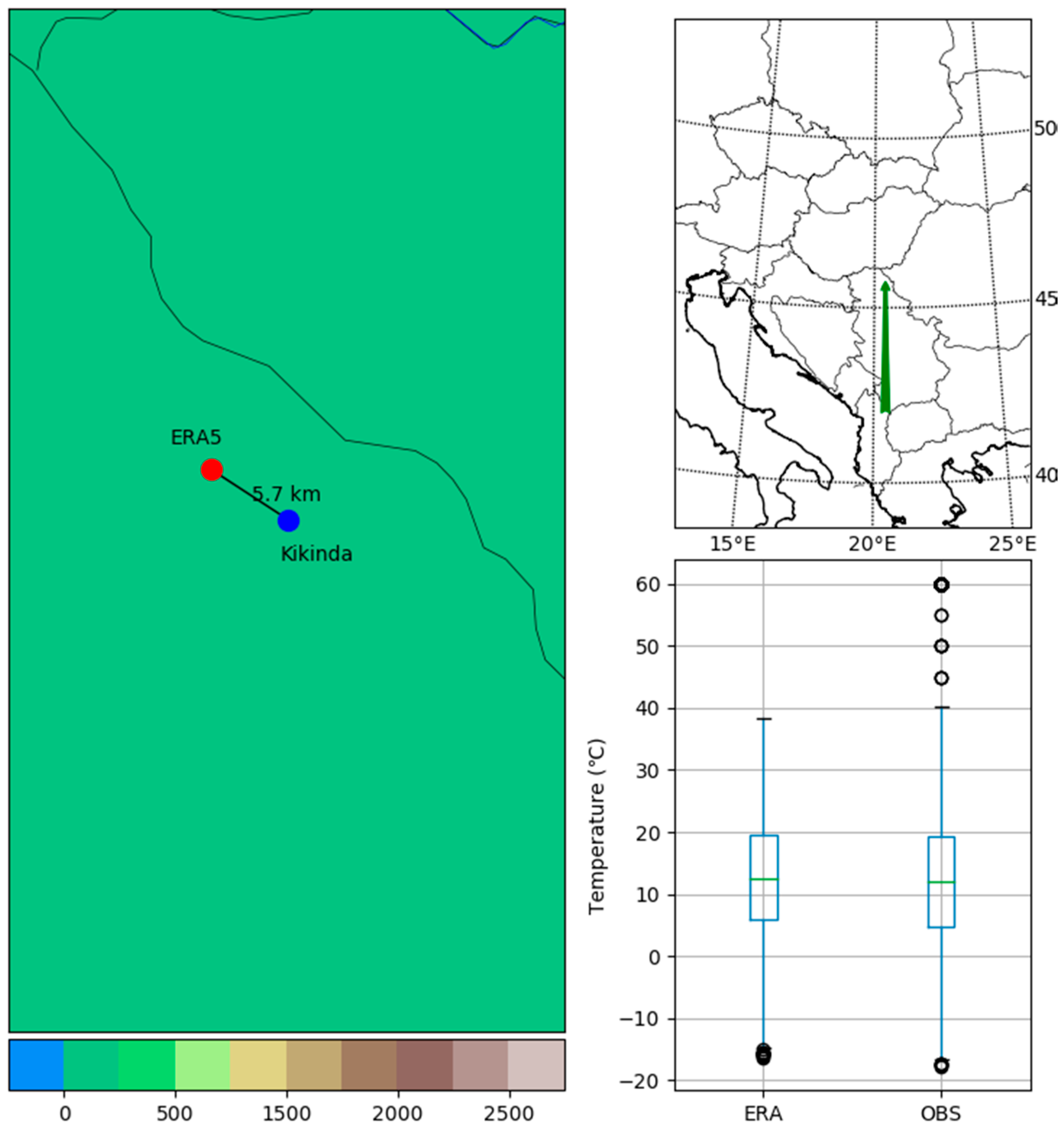
Lowland datasets were measured within the AWS network of the System of the Forecasting and Warning Service of Plant Protection of Serbia (PIS) (Novi Sad, Serbia). This AWS network was designed and set up to provide information about micrometeorological conditions in plant canopies, orchards, and vineyards to analyze the environmental conditions in which host plants and harmful organisms develop. The AWSs were equipped with sensors for the measurement of air and soil temperature, air relative humidity, soil moisture, precipitation amount, and leaf wetness duration. The temperature sensors were installed in fruit orchards, commonly at the mid-crown level (a height of approximately 1.2 m). All selected locations were in orchards situated in the Vojvodina (Northern Serbia) region, which is a part of the Pannonian lowlands (Figure 1). The data used in the study were measured during the 2014–2017 growing season (1 March–31 October).
The mountain dataset was measured at the Gumpenstein synoptic weather station within the network of the Zentralanstalt für Meteorologie und Geodynamik (ZAMG; Central Institute for Meteorology and Geodynamics) (Vienna, Austria). The Gumpenstein weather station is located in the Austrian province of Styria at an altitude of 700 m a.s.l. (Figure 2). The temperature measurements were made at a height of 2m in a standard meteorological shelter. Selected data series were measured during the 2014−2017 period. For the purpose of the study, the 01 May−30 November 2017 period was selected.
The desert dataset was measured in the el-Bahariya oasis in Egypt in the framework of the MosqDyn project AWS network. This AWS network was established and set up to monitor micrometeorological conditions and their suitability for the abundance and activity of local mosquito populations. The AWS was equipped with sensors for air temperature, precipitation, and relative humidity measurements. El-Bahariya is a depression and oasis in the Western Desert of Egypt located in the Giza Governorate. The oasis is situated 370 km southwest of Cairo. The valley hosts many guava, mango, and date groves and has a roughly oval shape covering an area of 2000 km². The sensors were installed at a height of 2 m in the northern part of the oasis (Figure 3).
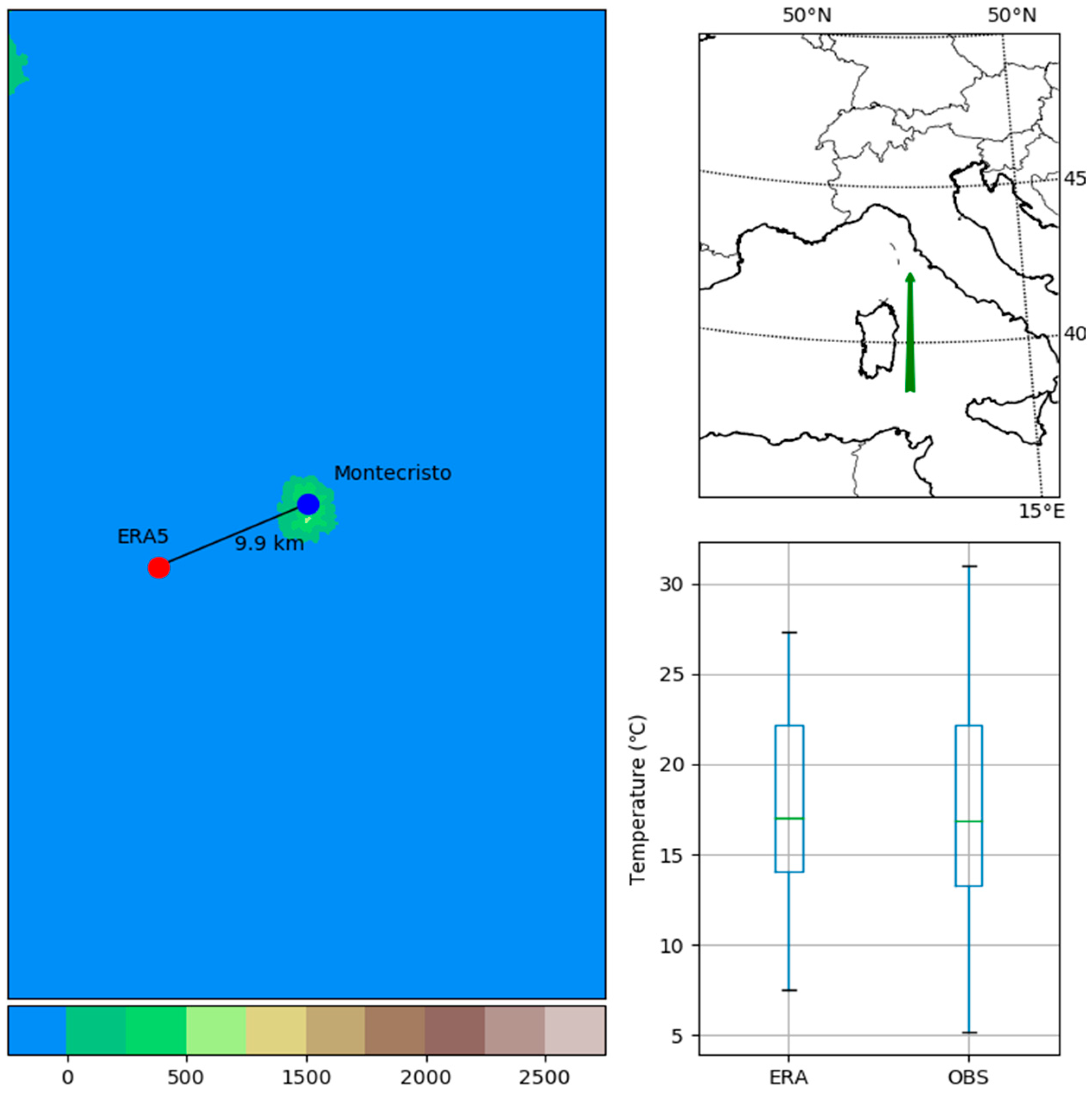
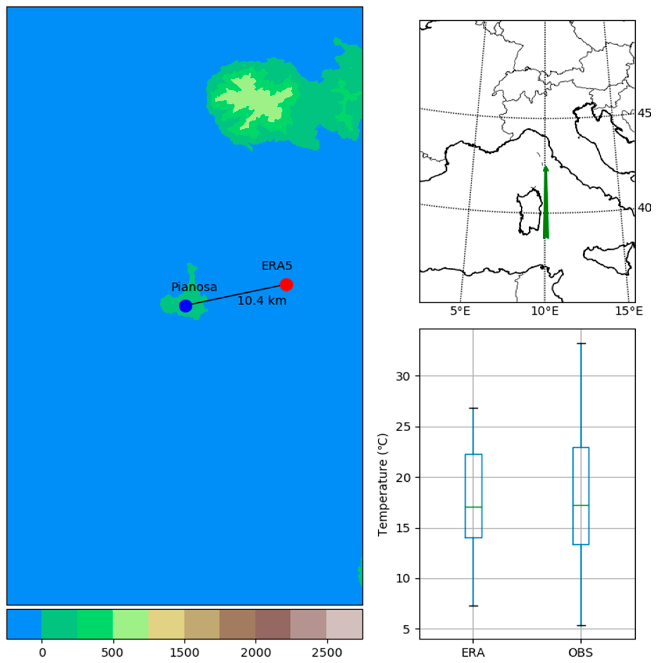
Island datasets were measured at the islands of Montecristo and Pianosa, Italy (Figure 4 and Figure 5) in the framework of the Environmental Modelling and Monitoring Laboratory for Sustainable Development (LAMMA) consortium activities [26]. Weather stations were located on stony elevated terrain that is highly exposed to atmospheric circulations and performed the following measurements: air temperature, humidity, wind direction, wind speed, precipitation, and the intensity of incoming solar radiation. Data used in this study were measured during the 1 May–15 November 2016 period.
2.2. Gap Filling Method Description
The designed gap filling method is based on the following assumptions:
- In the case of temperature data, due to the high autocorrelation of the time series, important information is contained within the time series before and after the gap [27]. Therefore, a portion of the time series that is not missing is used for the bias correction of ERA5 data;
- It is important to limit the amount of data used for the gap filling method (learning period) to avoid seasonal changes in temperature data; however, it is also important to use enough data to be able to exploit the high autocorrelation in the time series. The determination coefficient R2 was used to validate that enough data was present in the fitting process;
- Diurnal temperature biases [23] are recognized as a possible problem and new technique for filtering the learning data was applied to improve this methodology.
- To efficiently fill gaps in large datasets, a simple, fast, and reliable approach of linear regression was selected.
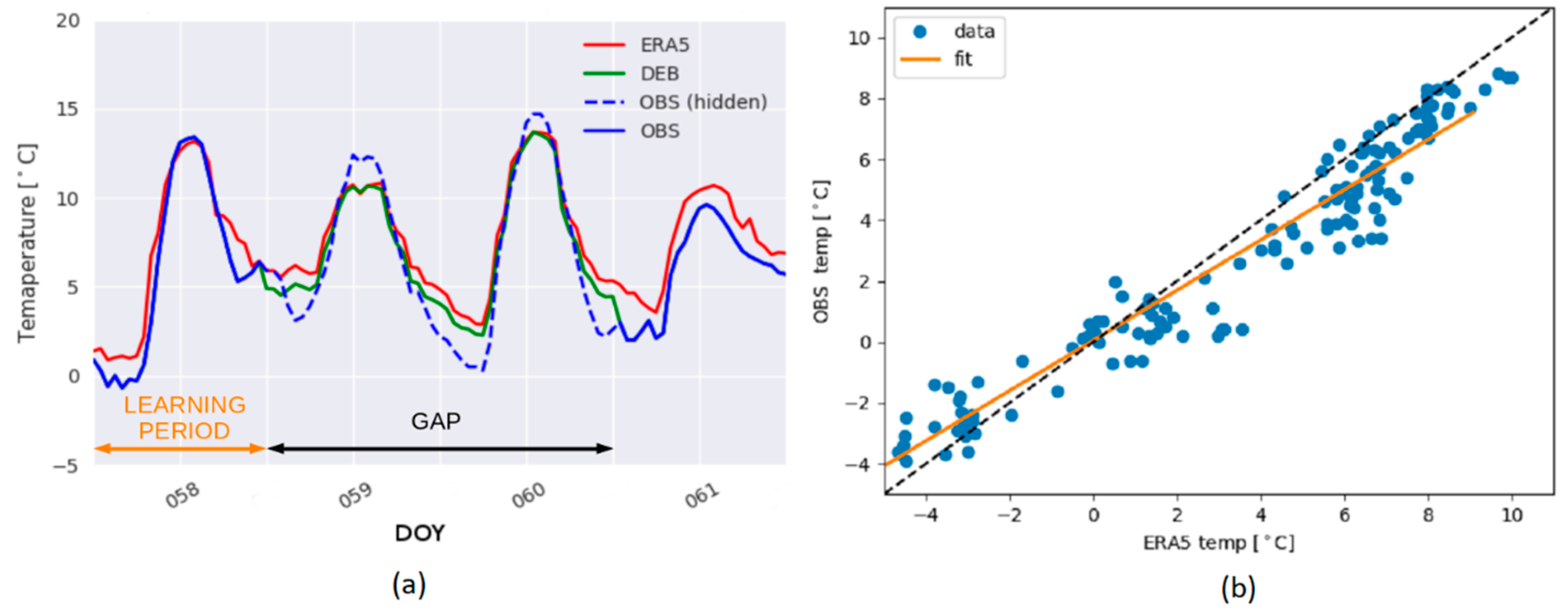
To fill the gaps in the time series, it was necessary to find the beginning of the gap and the gap length (shown in Figure 6a by the black left-to-right arrow). Gap filling was performed step by step by applying the debiasing technique for each missing observation in the gap period. Older missing observations were filled first. We proceeded step by step toward the gap end. During this process already filled values in the gap also influence the gap-filling process for later missing observations in the same gap.
To fill one missing observation in the gap, it was necessary to determine the relationship between the existing observations and the reanalysis for a certain period of time before the missing observation (learning period shown in Figure 6a by the orange left-to-right arrow). The learning period used in this study was 30 days and observations were hourly. The length of the learning period was chosen empirically so that it would be short enough not to be influenced by seasonal changes but long enough to contain an appropriate amount of data for linear regression.
Due to uncertainties in radiation, surface, and Planetary Boundary Layer (PBL) physics schemes in numerical models, diurnal variations in temperature biases can occur. To avoid this problem, a ± 3-h filter was applied to the time series. This way, data from the same part of the day were used. After reducingthe influence of the diurnal bias changes on the debiasing process with the filter, we calculated the linear regression coefficients (Figure 6b) and applied them to the reanalysis values for the missing observation time step.Thus, we reconstructed one-time step in the gap period. Linear regression was chosen as it is a computationally efficient and fast process that satisfies the requirements of this methodology.
3. Results
The described methodology was applied to all data sets for different gap lengths and seasons. To assess the effects of the bias correction, the bias score (B), expanded bias uncertainty (U(B)), and root mean square error (RMSE) were calculated for both ERA5-only (RMSEERA5) and ERA5-debiased (RMSEDEB)temperature gaps. Bias (B) is the systematic difference between a model predicted value (P) and a measured reference (M): . The expanded uncertainty U(B) is calculated as:
where k is the coverage factor and is the combined bias uncertainty which is calculated using the first-order uncertainty propagation formula in the following form [28]:
where u(P) and u(M) are the standard uncertainties of the predicted and measured values and PCC(P,M) is the Pearson’s correlation coefficient (PCC) which is calculated as the determination coefficient for all gap filling steps and for all experiment locations. More details about the expanded bias uncertainty (U(B)) calculation can be found in Appendix A, and plots of B and U(B), for all selected locations and gaps can be found in Appendix B.
D’Agostino and Pearson’s normality test [29,30] were used to estimate whether the dataset obeys a standard distribution, as the convergence factor of 1.96 is commonly used for normal Gaussian distributions or near-Gaussian distributions for the 95% confidence interval(CI). Since the tests showed that the data is not normally distributed, and for randomly selected parts of the dataset the skewness was above 1/3 and the kurtosis parameter values were negative, we could not calculate a variable coverage factor based on the distribution of each gap, and had to treat the distribution as non-normal and unknown. Therefore, the coverage factor was calculated from Chebyshev’s inequality giving k = 4.472 for the 95% CI [31].
Site-specific analysis was performed using RMSEDEB values, the differences between RMSEDEB and RMSEERA5 and the standard deviation of the observed data used for bias correction (Figures 7–12 and 14–16) as well as the bias and bias uncertainties calculated for each location (Figure A1, Figure A2, Figure A3, Figure A4 and Figure A5).
3.1. Lowland Data Sets
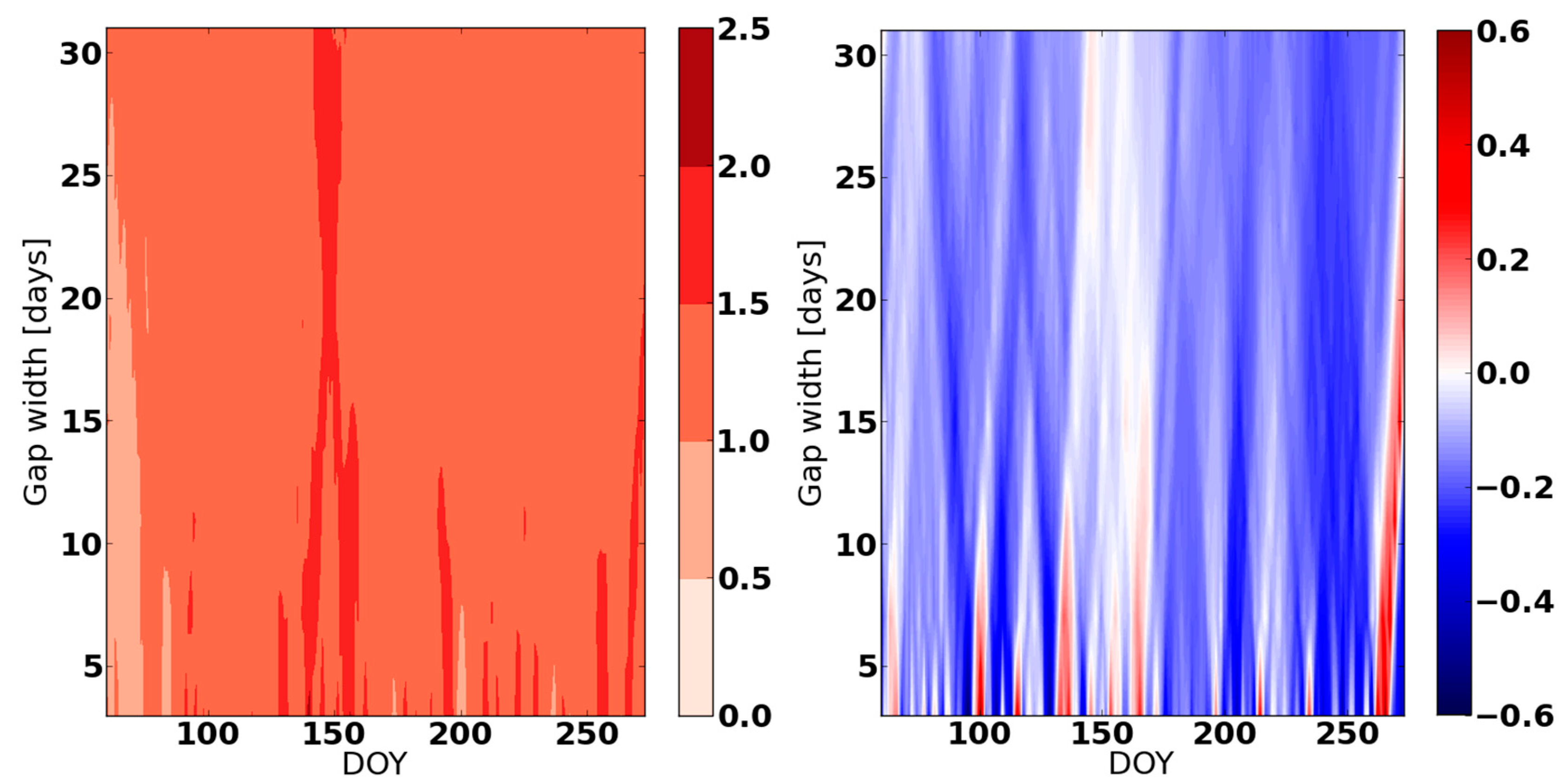
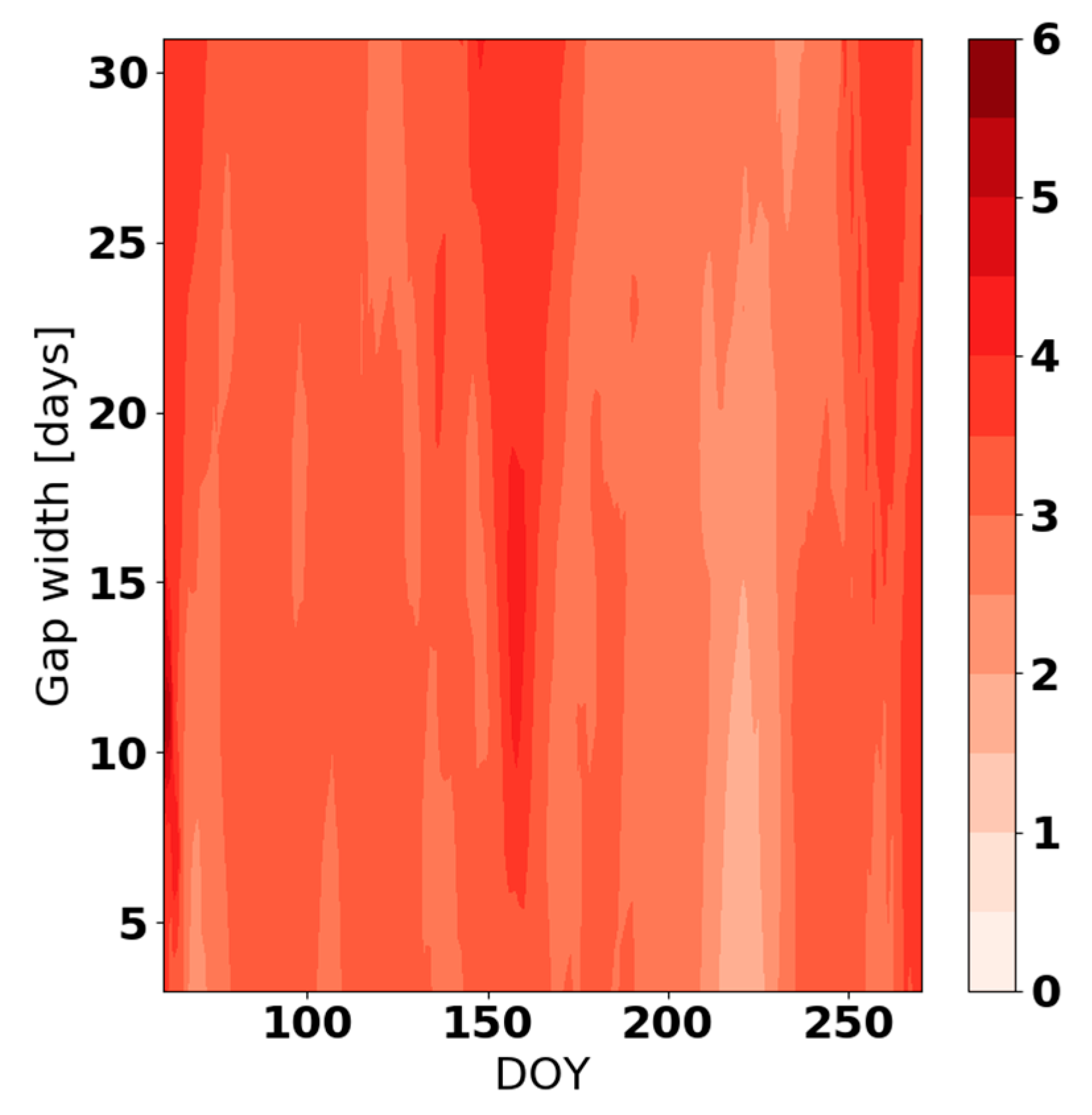
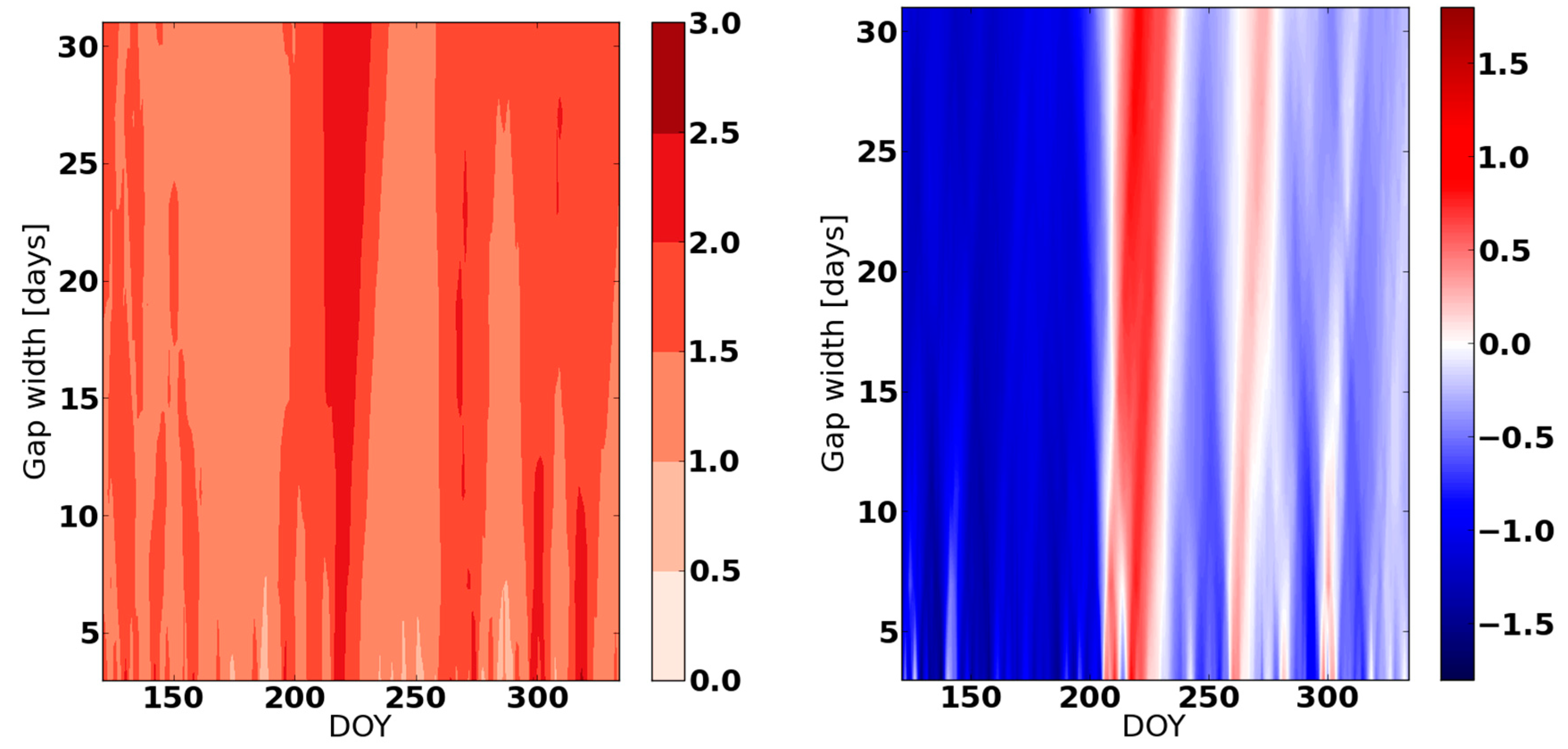
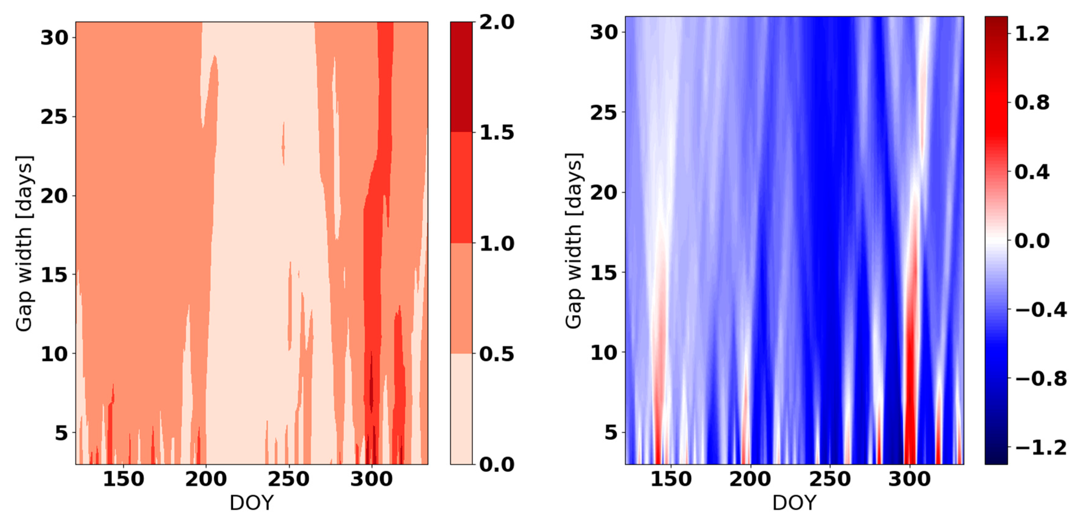
The RMSEDEB values varied between 0.5 and 2 °C, with commonly high values for up to 5-day gap lengths. Although the blue-dominated plot in the right panel of Figure 7 indicates that the debiased dataset produced lower RMSE values than the ERA5-only dataset, some red areas associated with gaps that were better filled by ERA5-only data are present in the figure. A possible source of this effect is indicated by the standard deviation of the observed data (Figure 8), as periods with relatively high standard deviations (more than 5 °C) can be identified beginning in March (DOY 50–65) and from the end of May until the end of June (DOY 142–182). During both indicated periods, positive bias (Figure A1) indicates that both data sets overestimate measurements; however, it is more pronounced for ERA5-only data. During the growing season (DOY 92–275), the highest bias uncertainties are obtained in the middle of the season when temperatures are highest as well as the exchange of energy and water vapour fluxes between canopy and atmosphere. An air temperature sensor was installed at a height corresponding to the middle of the crown, apple growth was an important factor affecting the variation in the measured air temperature; specifically, when the first leaves appeared (in March), they strongly affected the energy balance of the canopy by increasing the latent heat flux and energy absorbed and emitted by the leaves. Consequently, this affected the canopy air temperature and its variation over the period of intensive plant area development. When crowns formed (in May), the weekly or monthly variation in air temperature caused synoptic-scale atmospheric processes. In that period, intensive or sudden (“squall”) winds could instantaneously affect air temperature by increasing air canopy mixing, increasing the variation and standard deviation of the measured air temperature at the hourly scale. Since wind speed measurements were not performed at this location, we can suppose that this is the cause of the increase (albeit impermanent) in the standard deviation during the DOY 142–182 period for gap filling.
3.2. Mountain Data Sets
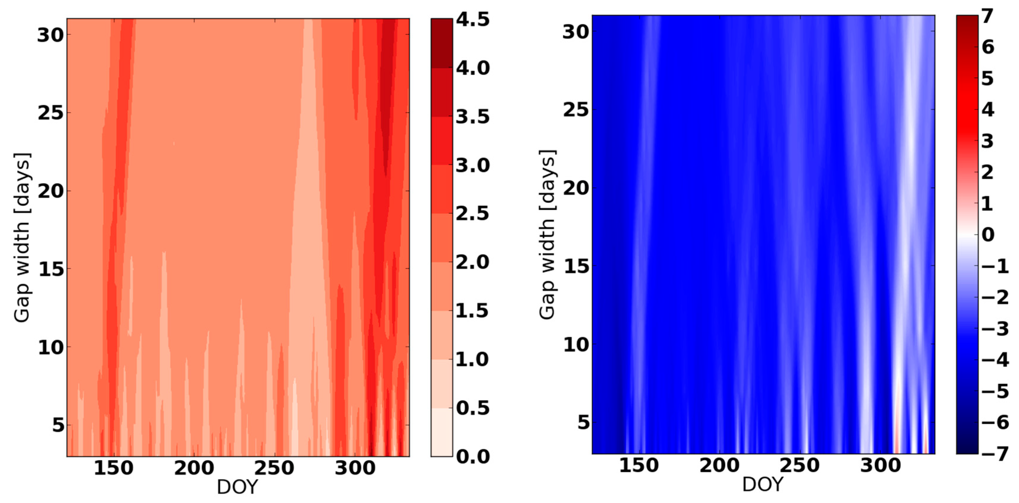
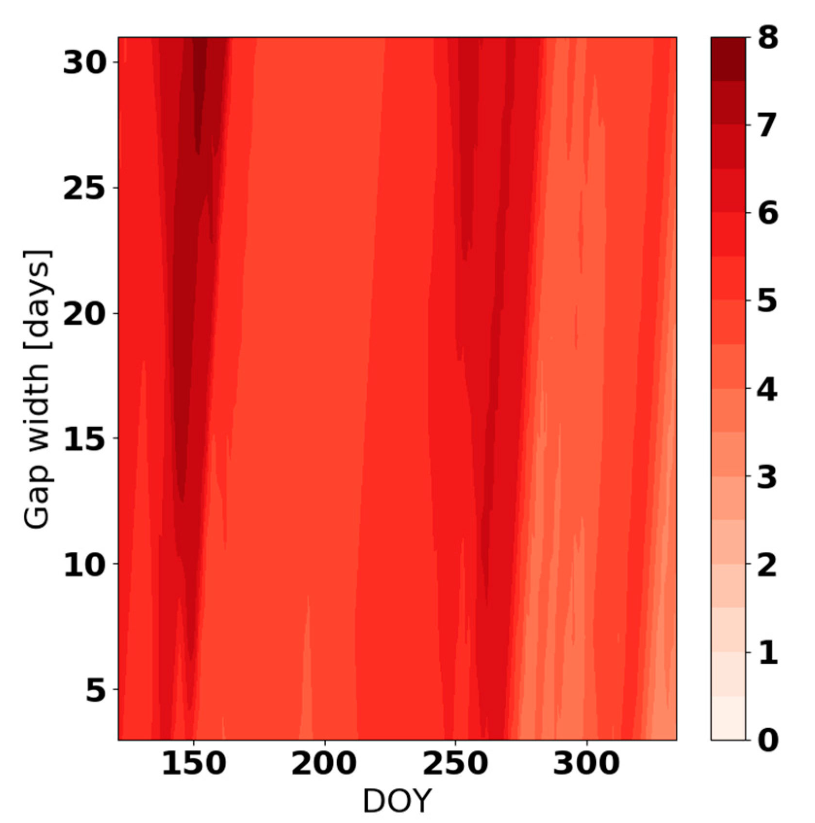
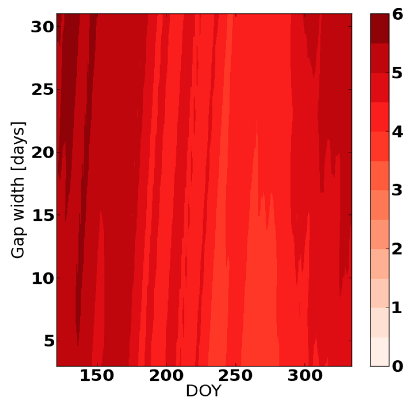
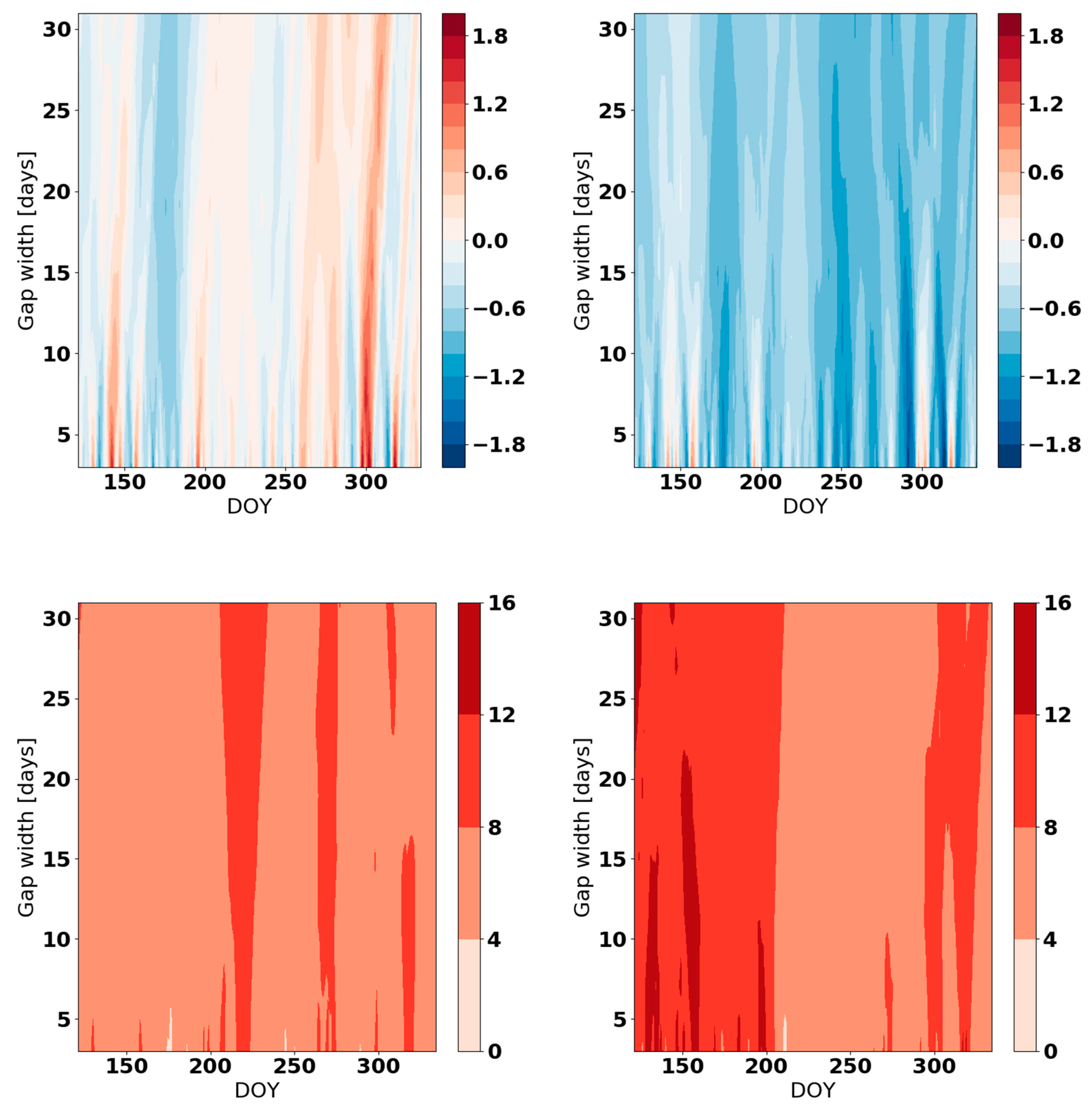
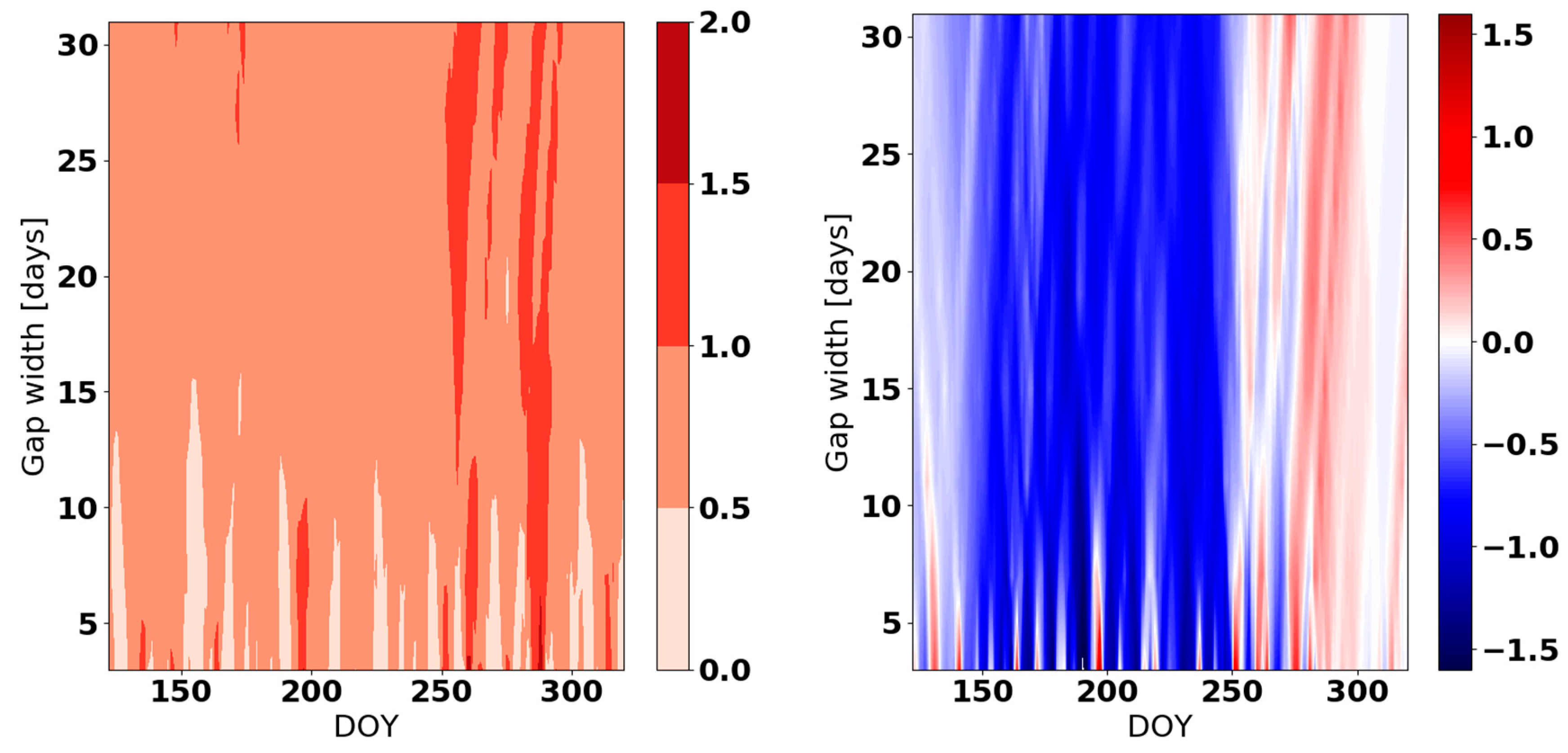
The superiority of the debiasing technique was expected in the case of Gumpenstein station. Figure 2 and Table 1 clearly show that the ERA5 point for this location was 380 m higher in the Alps, which is the result of the sub grid scales of the flat areas where the Gumpenstein AWS is located and the applied parameterization of sub grid-scale processes. Therefore, significant temperature differences between the observations and reanalysis were expected. The obtained bias for ERA5-only data (Figure A2) is more than 6 °C higher than for ERA5-debias data, while bias uncertainties for the debiased data set are much lower for all gap lengths. An interesting increase of bias uncertainty during the cold part of the year can be connected with late and early snowfall in mountains, which can affect temperature measurements and the accuracy of model simulations. High RMSEDEB at DOY 150 (Figure 9, left panel) is partly result of high standard deviation of observed data (Figure 10) which were used for bias correction. Differences in RMSE decreased towards winter (Figure 9), since the vertical temperature gradient in the Alps decreases from April to December [32]. Exceptions to this trend occurred in DOY 320–321 and DOY 327–329, when heavy snowing affected measurements and increased the standard deviation of measured data over 2017.
3.3. Desert Data Sets
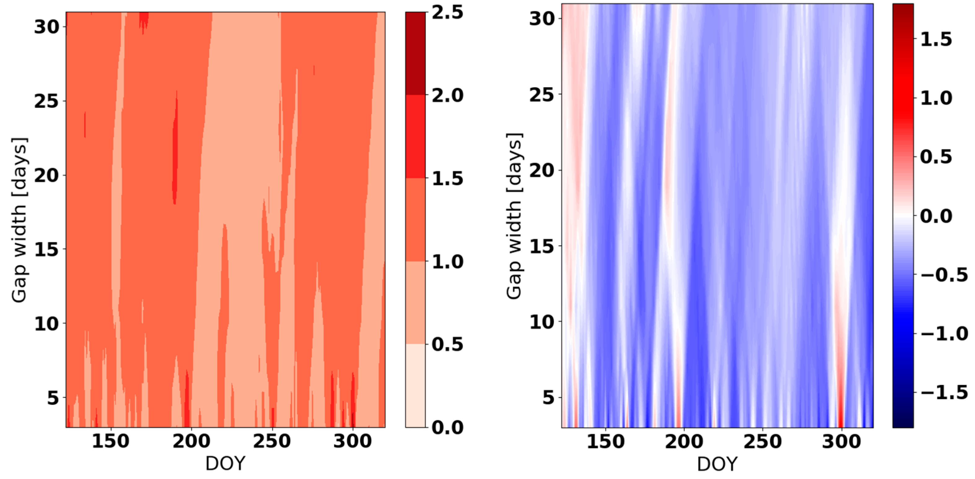
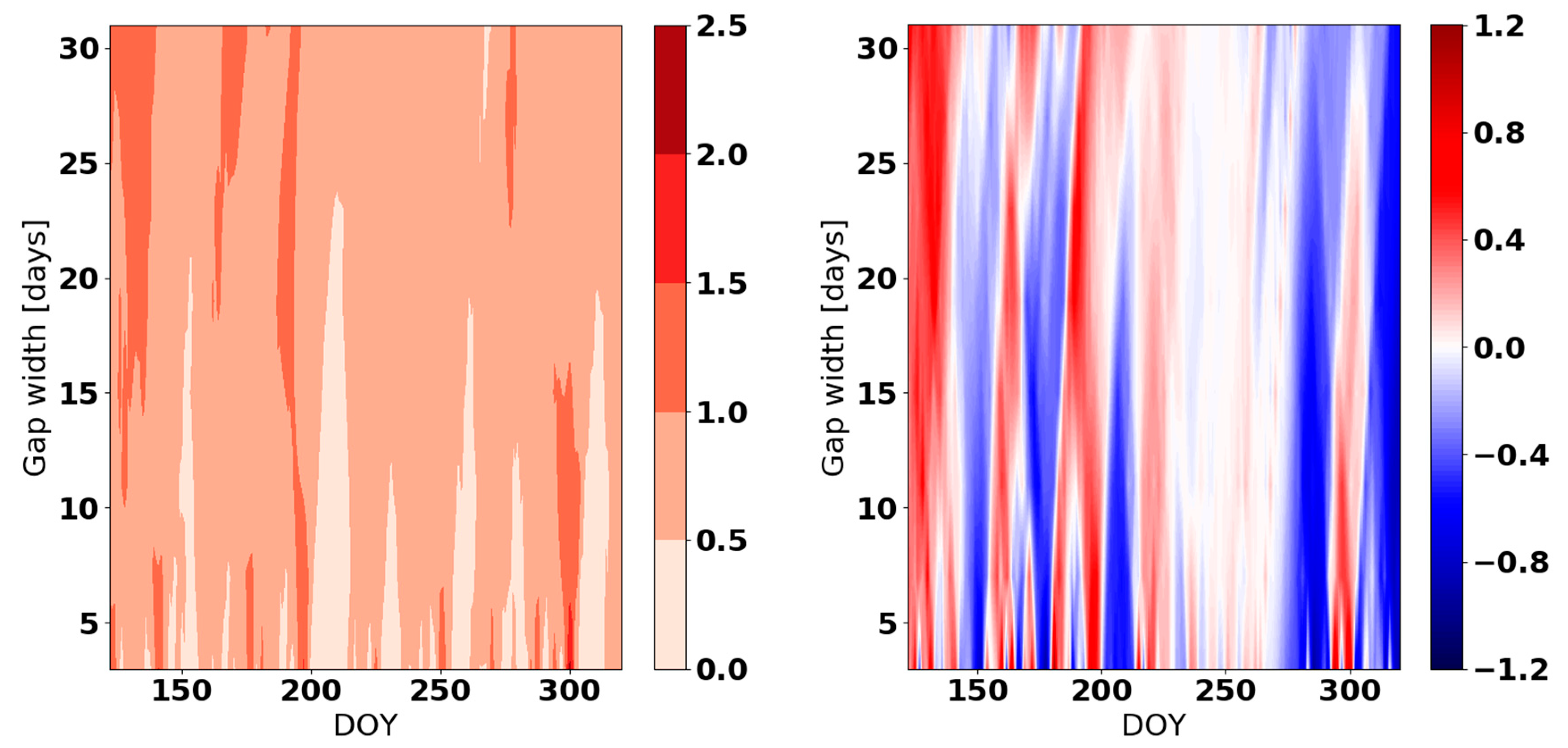
During the prevailing part of the period of interest, the applied bias correction gap-filing technique provided better results than the ERA5-only data (Figure 11) with significantly lower bias and bias uncertainty for all gap widths (Figure A3). However, there were some exceptions to this tendency, which deserve our attention. The desert landscape surrounding the Bahariya oasis AWS is very uniform (see Figure 3), with neither mountains nor significant vegetation to serve as a source of uncertainties in the ERA5 reanalysis. However, the constant inflow of desert air can produce significant variation in air temperature at an hourly time scale. Figure 12 clearly shows that a high standard deviation of the bias correction data for gaps between DOY 120 and DOY 172 corresponded to a high daily variation in air temperature (Figure 13). During September (DOY 250–275) and at the end of the year (after DOY 300), the variability in the daily amplitude was significant, ranging from 7.4 °C to 22.6 °C. This variability affected the bias correction procedure, particularly during the DOY 216–228 period when ERA5 obviously better reproduced the observed air temperature. During this period and the small time window in September, the bias uncertainty of ERA5-only data was lower than that of the debiased data set.
3.4. Island Data Sets
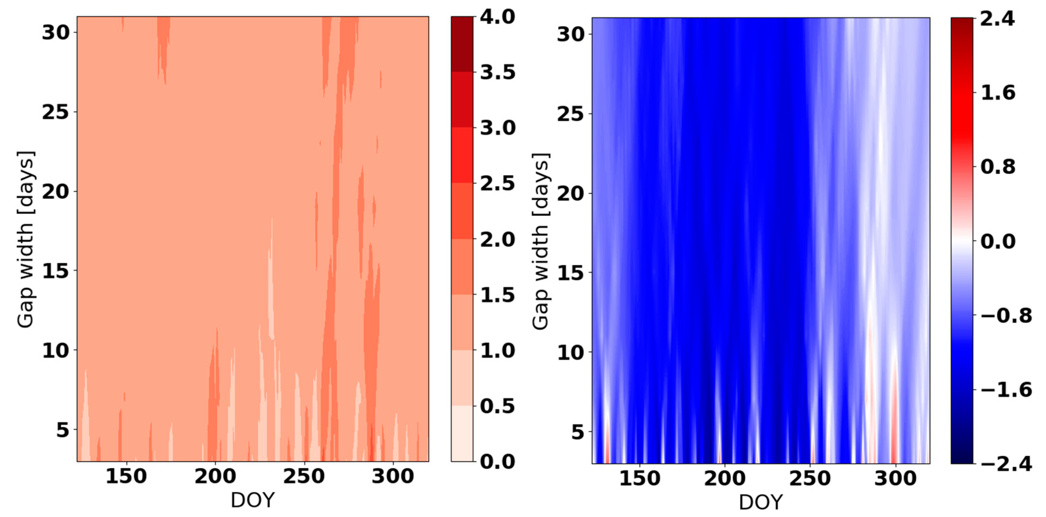
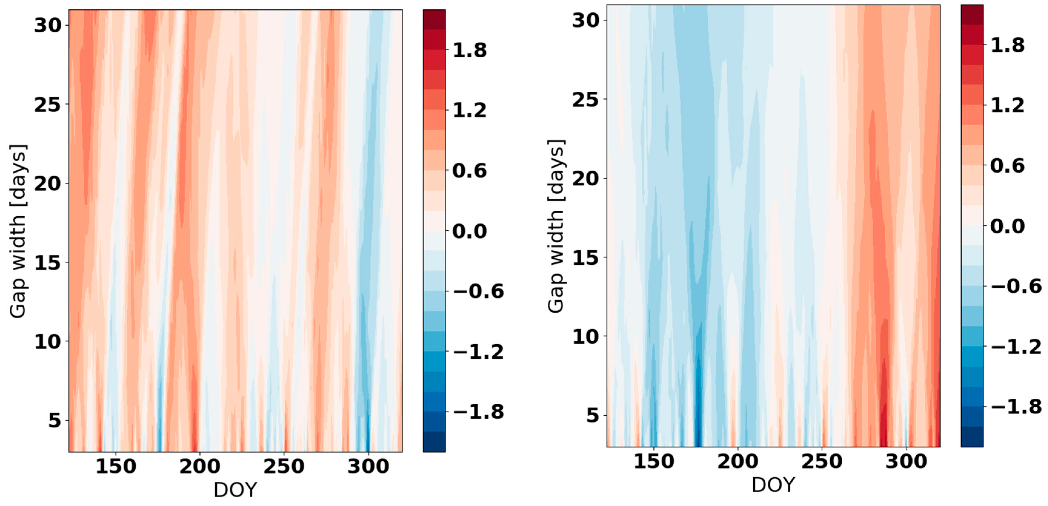
Due to the fact that the heat capacity of water is much higher than that of land, the air temperature variation above the sea surface was always much lower than that above land in the study period. Additionally, the daily and annual variation in air temperature above coastal areas and islands was much lower than above far-inland territories. Therefore, it is not surprising that there was a low and uniform (at the annual level) standard deviation in the observed data used for gap filling (Figure 14) for both Montecristo (2.3–2.8 °C) and Pianosa (2.5–2.7 °C) islands. With respect to the ERA5 mean orography, grid cells in which both islands were located were represented by water (Figure 4 and Figure 5), implying a low variation of reanalysis temperature. The last two circumstances demonstrate the high efficacy of the debiasing technique (Figure 15 and Figure 16, left panels) and low differences between RMSEDEB and RMSEERA5 (Figure 15 and Figure 16, right panels). According to the results presented in Figure A4 and Figure A5, the debiased data set slightly overestimates measurements in the spring and underestimates them in autumn. In the case of ERA5-only data, the situation is exactly the opposite. However, in both locations, bias uncertainty is lower, for all gaps, for debiased data sets than for ERA5-only data sets.
4. Discussion
The gap-filling methodology test results indicate that the presented ERA5-debiasing technique has different efficacies that vary with respect to location, gap width, and the standard deviation of the observed data used for bias correction. However, high values of the Pearson’s r coefficient and p-values below 0.05 (Table A1) for all locations and gap lengths indicate a strong linear relationship between ERA5 and the observed data used for gap filling and debiasing.
Overall, mean bias uncertainty and mean RMSE for all gap widths and all DOY are provided in Table 2. It is evident that the new technique significantly decreases bias, bias uncertainty, and root mean square error. The only exception is for Montecristo, for which ERA5 already had a small bias, and therefore the new technique wasnot able to improve the results here.
Particularly important is the propagation of standard uncertainties of input data (predicted and measured air temperature) (Table A2, Appendix A) towards gap bias. The comparison of the standard uncertainty of input data (Table A2) and mean bias uncertainty (Table 2) indicates that U(B) for debiased data is much closer to the uncertainty of input data than in the case of ERA5-only data.
The lowest average RMSEDEB was obtained for island locations (Montecristo = 1.06 °C, Pianosa = 1.26 °C), and the highest average RMSEDEB was obtained for mountain regions (Gumpenstein = 1.88 °C), as was expected according to the elaborated ERA5 reanalysis performances and standard deviations of the observations.
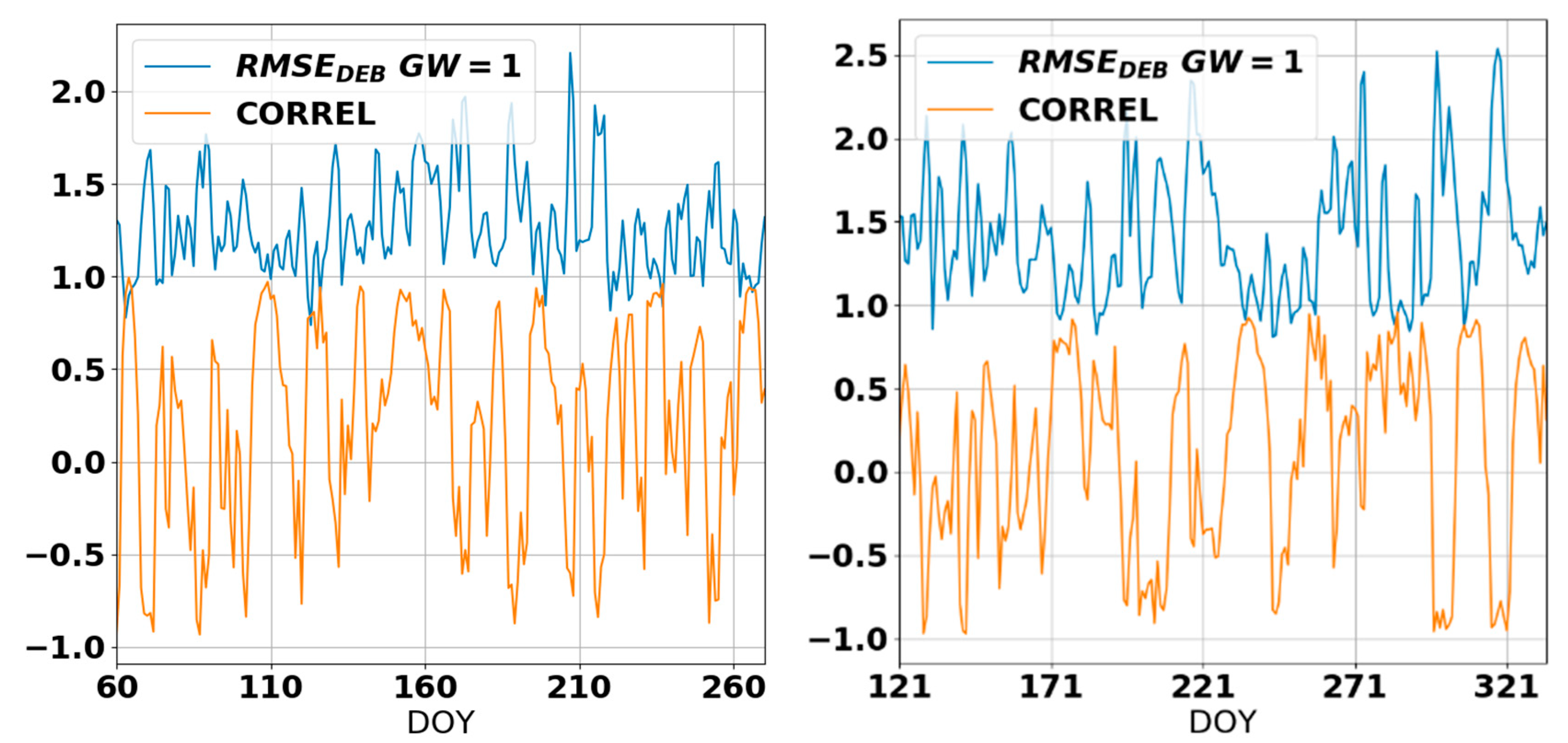
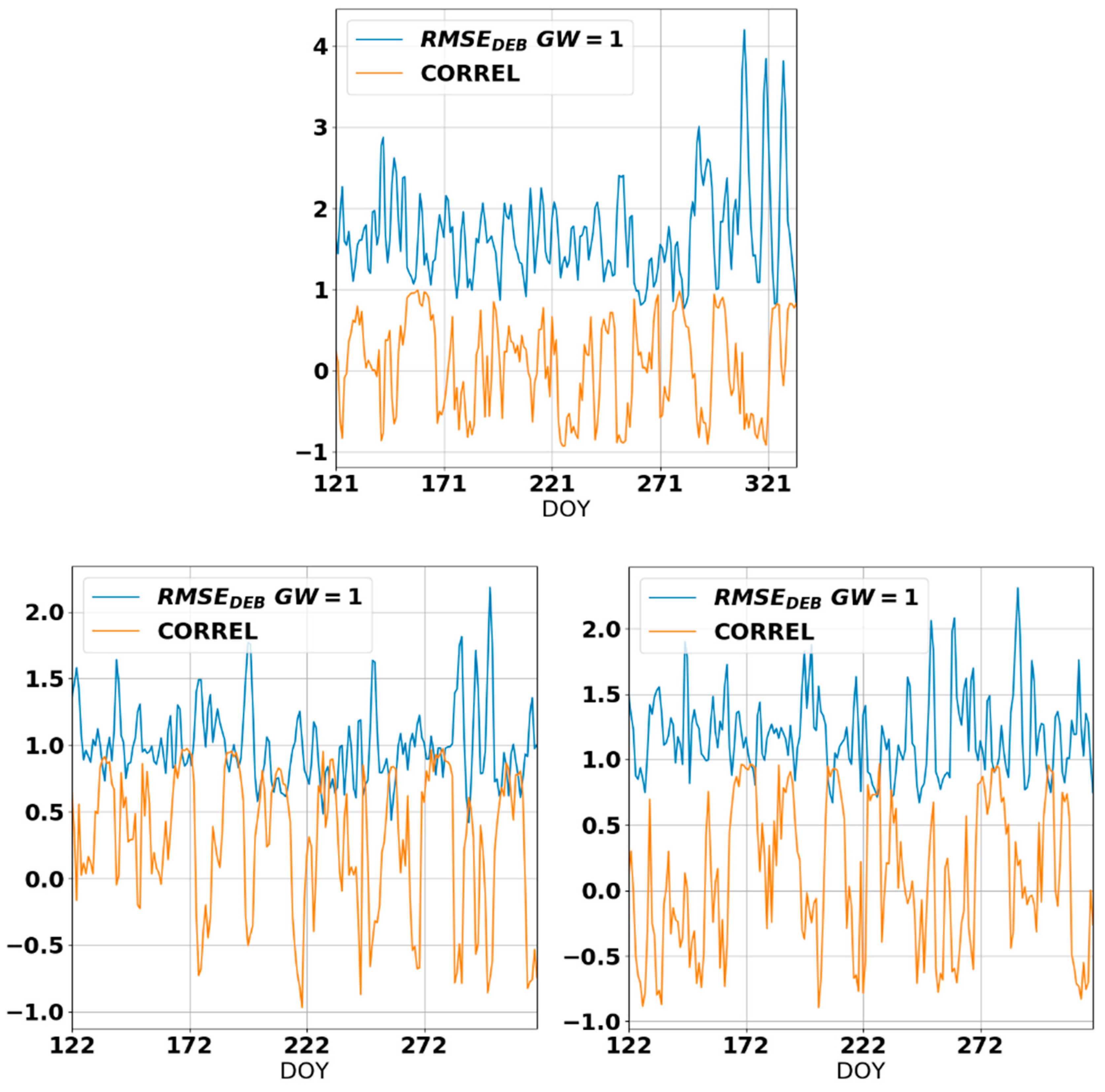
However, the high RMSEDEB in the case of small gaps has drawn our attention. For all examined locations, we identified strong correlations (r > 0.7) between the standard deviation of the observed data used for linear regression and RMSEDEB (Figure 17). The Pearson’s product-moment correlation coefficient is the test statistic that was used to measure this relationship together with the standardized criteria suggested by Evans [33] for estimating the strength of association. More specifically, we obtained high negative correlations for high RMSEDEB values and high positive correlations for low RMSEDEB values. At a seasonal scale, the correlation among curves was between −0.61 (Montecristo) and −0.60 (Kikinda), indicating a medium-intensity but stable correlation for all locations (Bahariya = −0.56, Gumpenstein = −0.37, Pianosa = −0.27).
We performed a detailed analysis of the measured data used for linear regression and the calculated data for gap filling with respect to the scale of the gap to identify the cause of such systematic behavior. The obtained results lead to the conclusion that RMSEDEB decreases when the standard deviation of the observed data increases with the gap width since for larger standard deviations, the interval of the observed values used for debiasing is broader. Accordingly, in further applications of this technique, it will be important to consider that the standard deviations of measured air temperatures are a result of meteorological and other environmental (the presence and development of plants, high mountains, deserts, and large water bodies) conditions, however the variation in RMSEDEB with standard deviation is the result of the applied calculation methodology.
In some exceptional situations, such as in Bahariya (DOY 216–228), the ERA5 deviation from measurements was reduced on a daily basis, producing a much better gap filling performance with the ERA5-only dataset. This could be linked to the observed seasonal shift in the variance and amplitude of the diurnal temperature range. The amplitude was high throughout the year, which is typical of a hot desert climate [34]. However, the variance in the diurnal range was much higher for autumn and spring than for other seasons, leading to a significantly smaller bias for ERA5 during the JJA June–August period. Similar behavior has been observed for ERA-Interim and ERA-40 reanalyses [35].
Finally, we discuss the merit of the presented gap-filling technique in performing daily data series. Even though the goal of this study is to develop and test the technique for filling gaps in hourly temperature data series, the analysis is fully justified since users demands are commonly related to daily weather data. At all locations and for all gap scales, the maximum RMSEDEB calculated using daily data (Table 3) is smaller in comparison to results obtained using hourly data. A lower RMSEDEB of daily temperature time series for different gap lengths and locations can be noticed in Figure A6, Figure A7, Figure A8, Figure A9 and Figure A10 (left panels). However, differences between RMSEDEB and RMSEERA5 are less pronounced for daily data except in the case of Gumpenstein (Table 3), where the maximum deviation for daily data is the highest. Almost the same results for (RMSEDEB-RMSEERA5) are obtained using hourly and daily gap-filling data (Figure A7, right panel), which clearly indicates that there is systematic deviation of ERA5 data from measurements.
Average RMSEDEB values obtained using hourly temperatures (Kikinda = 1.3 °C; Gumpenstein = 1.9 °C; Bahariya = 1.5 °C; Montecristo = 1.1 °C and Pianosa = 1.4 °C) are in the same range (1.5–2.0 °C) as those obtained by Chen et al. [32] for missing data values for daily temperature for the United States using a self-calibrating data quality control and which are described as “impressively low average”.
There are many fully statistical self-calibrated estimation methods (for example, Chen et al. [36]) as well as spatial, temporal, and spatio-temporal methods [2] that work very well. However, extreme weather events and high daily amplitudes of air temperature will become the new climate norm for many places in the world in the future. It is difficult for statistical techniques to infer data far from observations points. Therefore, we developed and tested gap-filling methods, that include dynamical and statistical concepts.
5. Conclusions
The presented technique and testing results offer a new methodology for gap filling based on a combined dynamical-statistical methodology that differs from the common statistical methods widely reported in the literature. Results obtained indicate that in the case when measured data are not available, ERA5 data can be used for temperature gap filling. However, in cases when the ERA5 grid point significantly deviates from the observation point, particularly on high mountains, debiasing of ERA5 data based on observations is necessary in order to obtain useful temperature data. Testing in different landscapes (from desert to mountains) and world regions (from subtropical latitudes to midlatitudes) addresses region-specific uncertainties that should be taken into account in further applications of this technique. The next step will be testing the presented concept for soil temperature and air humidity data gaps.
The goal of this study is to enhance climate change and weather data-related studies which rely on long term data series. The complete procedure of technique application andprogram installation and running will be posted on the H2020 SERBIA FOR EXCELL project web page (www.serbiaforexcell.com) until the end of 2018.
Supplementary Materials
The following are available at: https://www.mdpi.com/2073-4433/10/1/13/s1. Example Python code for gap filling and debiasing procedure and supplementary data.
Author Contributions
M.L. performed all coding and a major part of calculations, maps, plots, and error analysis, and contributed to writing; B.L.; analyzed requirements of AWS network gap filling, wrote a major part of the paper, and provided funds for open access publishing; L.D. designed solutions and contributed to calculation and writing; M.P. provided data for Bahariya station, contributed to calculation and writing. All authors contributed to the results discussion.
Funding
The research work described in this paper was realized as a part of the project ‘Studying climate change and its influence on the environment: impacts, adaptation and mitigation’ (III43007) funded by Ministry of Education, Science and Technological Development of the Republic of Serbia. This paper is supported by the SERBIA FOR EXCELL project which has received funding from the European Union’s Horizon 2020 research and innovation programme under grant agreement no. 691998.
Acknowledgments
The research work described in this paper was realized as a part of the project ‘Studying climate change and its influence on the environment: impacts, adaptation and mitigation’ (III43007) funded by Ministry of Education, Science and Technological Development of the Republic of Serbia. This paper is supported by the SERBIA FOR EXCELL project which has received funding from the European Union’s Horizon 2020 research and innovation programme under grant agreement no. 691998. The authors would like to thank Dr Anna Dalla Marta (UNIFI, Italy) and Prof. Josef Eitzinger (BOKU, Austria) for supplying temperature data. The measurements for the el-Bahariya Oasis (Egypt) was carried out under the MosqDyn project of the Belgium government led by Avia-GIS.
Conflicts of Interest
The authors declare no conflict of interest.
Appendix A
For calculating the expanded uncertainty U(B): First, we determined the input estimates for each input quantity: (mean ERA5 predicted 2m temperature), (mean DEBIAS predicted 2 m temperature), and (mean measured 2 m temperature) (. Where the (n − 1) degrees of freedom depend on the size of the gap (n is the number of observations in the gap). Second, we evaluated the standard uncertainty for each input estimate using a Type A evaluation (Table A1). The standard uncertainty of the input estimates is defined as the standard deviation:
The same is done for . Third, we calculated the covariances for all pairs of input estimates (significant correlations). We express the covariance as , where is the Pearson correlation coefficient. Fourth, we calculated the output estimate for ERA5 and DEBIAS as the difference between the predicted and measured value. Fifth, we determined the combined standard uncertainty of the bias, using the first order uncertainty propagation formula [28]:
In our case, the sensitivity coefficients . Sixth, we multiplied the combined uncertainty with the coverage factor () to obtain the expanded uncertainty U(B) and estimate the uncertainty interval .

Table A1.
Pearson r coefficient and p-value for ERA5 and measured data used for gap filing for DOY and gaps.
Table A1.
Pearson r coefficient and p-value for ERA5 and measured data used for gap filing for DOY and gaps.
| Pearson r | p Value | |||||||
|---|---|---|---|---|---|---|---|---|
| Min | Mean | Median | Max | Min | Mean | Median | Max | |
| Kikinda | 0.896 | 0.950 | 0.955 | 0.979 | 9.18 × 10−77 | 2.24 × 10−40 | 1.31 × 10−55 | 2.85 × 10−38 |
| Bahariya | 0.730 | 0.904 | 0.914 | 0.966 | 7.02 × 10−63 | 1.52 × 10⁻¹² | 1.72 × 10−38 | 1.83 × 10⁻¹⁰ |
| Gumpenstein | 0.762 | 0.889 | 0.894 | 0.957 | 4.01 × 10−36 | 7.66 × 10⁻¹⁰ | 8.25 × 10⁻²⁵ | 1.07 × 10⁻⁷ |
| Montecristo | 0.707 | 0.834 | 0.846 | 0.912 | 9.93 × 10⁻²⁸ | 5.80 × 10⁻¹⁰ | 3.75 × 10⁻¹⁸ | 3.49 × 10⁻⁸ |
| Pianosa | 0.545 | 0.760 | 0.747 | 0.939 | 5.69 × 10−36 | 0.002 | 1.83 × 10⁻⁹ | 0.029 |
Table A2.
Input estimates and standard uncertainties.
| Input Quantity | Description | Location | Input Estimate | Standard Uncertainty | Pearson r | Measurement Unit | Type of Evaluation |
|---|---|---|---|---|---|---|---|
| M | Measured two-meter temperature | Kikinda | 17.2 | 5.2 | °C | A | |
| Gumpenstein | 12.8 | 4.4 | °C | A | |||
| Bahariya | 27.2 | 5.5 | °C | A | |||
| Montecristo | 21.3 | 1.9 | °C | A | |||
| Pianosa | 22.0 | 2.4 | °C | A | |||
| Predicted two-meter temperature (ERA5 reanalysis) | Kikinda | 17.6 | 4.4 | 0.966 | °C | A | |
| Gumpenstein | 8.4 | 4.3 | 0.849 | °C | A | ||
| Bahariya | 26.4 | 5.1 | 0.940 | °C | A | ||
| Montecristo | 21.3 | 1.1 | 0.753 | °C | A | ||
| Pianosa | 21.3 | 1.1 | 0.562 | °C | A | ||
| Predicted two-meter temperature (DEBIAS) | Kikinda | 17.2 | 5.1 | 0.969 | °C | A | |
| Gumpenstein | 13.3 | 4.2 | 0.905 | °C | A | ||
| Bahariya | 27.1 | 5.4 | 0.961 | °C | A | ||
| Montecristo | 21.6 | 1.6 | 0.854 | °C | A | ||
| Pianosa | 22.3 | 2.1 | 0.862 | °C | A |
Appendix B
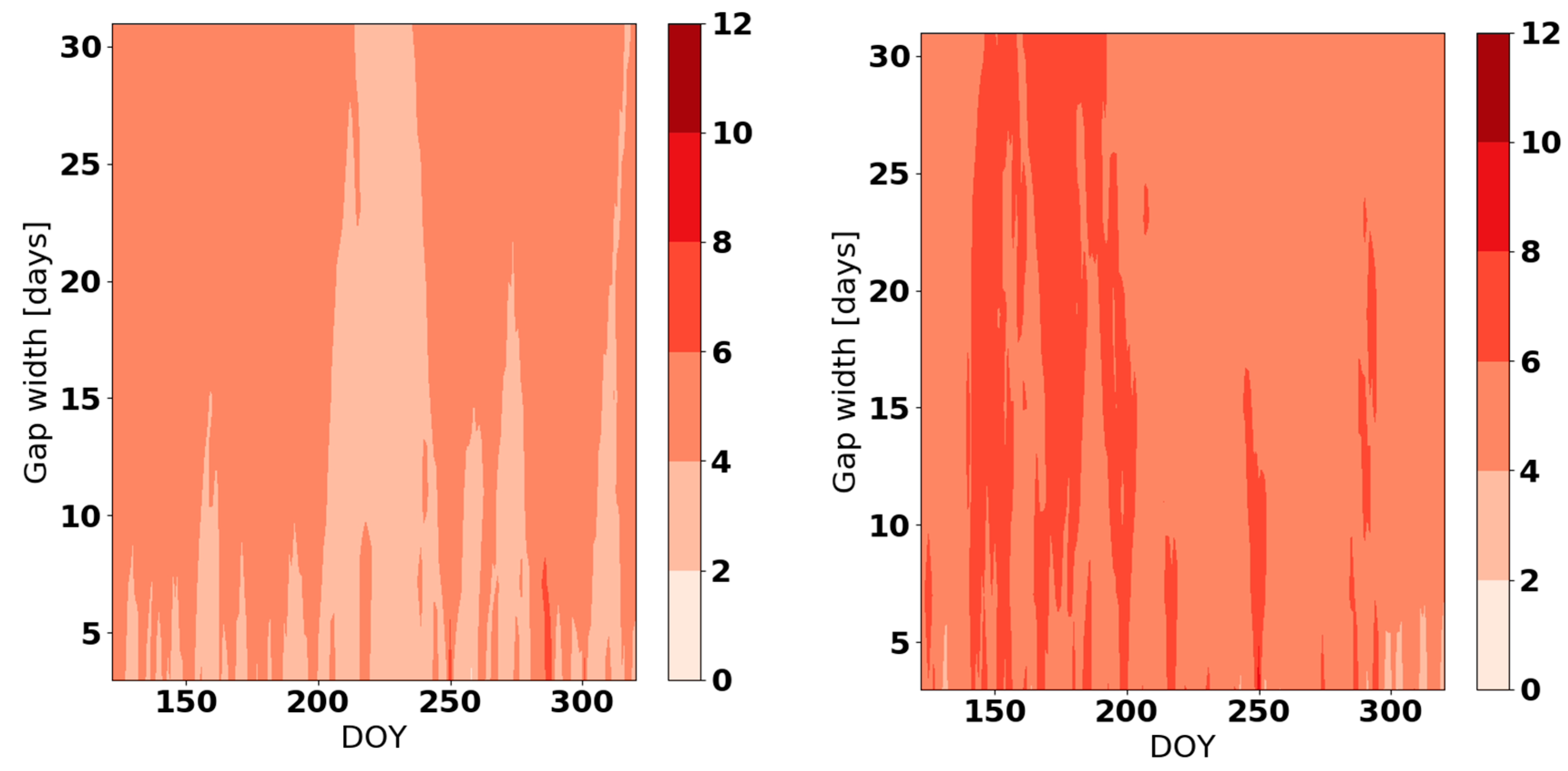
Figure A1.
BDEB (top, left panel), BERA5 (top, right panel), U(B)DEB (bottom, left panel), and U(B)ERA5(bottom, right panel) calculated using data for DOY 60-273 2014 in Kikinda.
Figure A1.
BDEB (top, left panel), BERA5 (top, right panel), U(B)DEB (bottom, left panel), and U(B)ERA5(bottom, right panel) calculated using data for DOY 60-273 2014 in Kikinda.

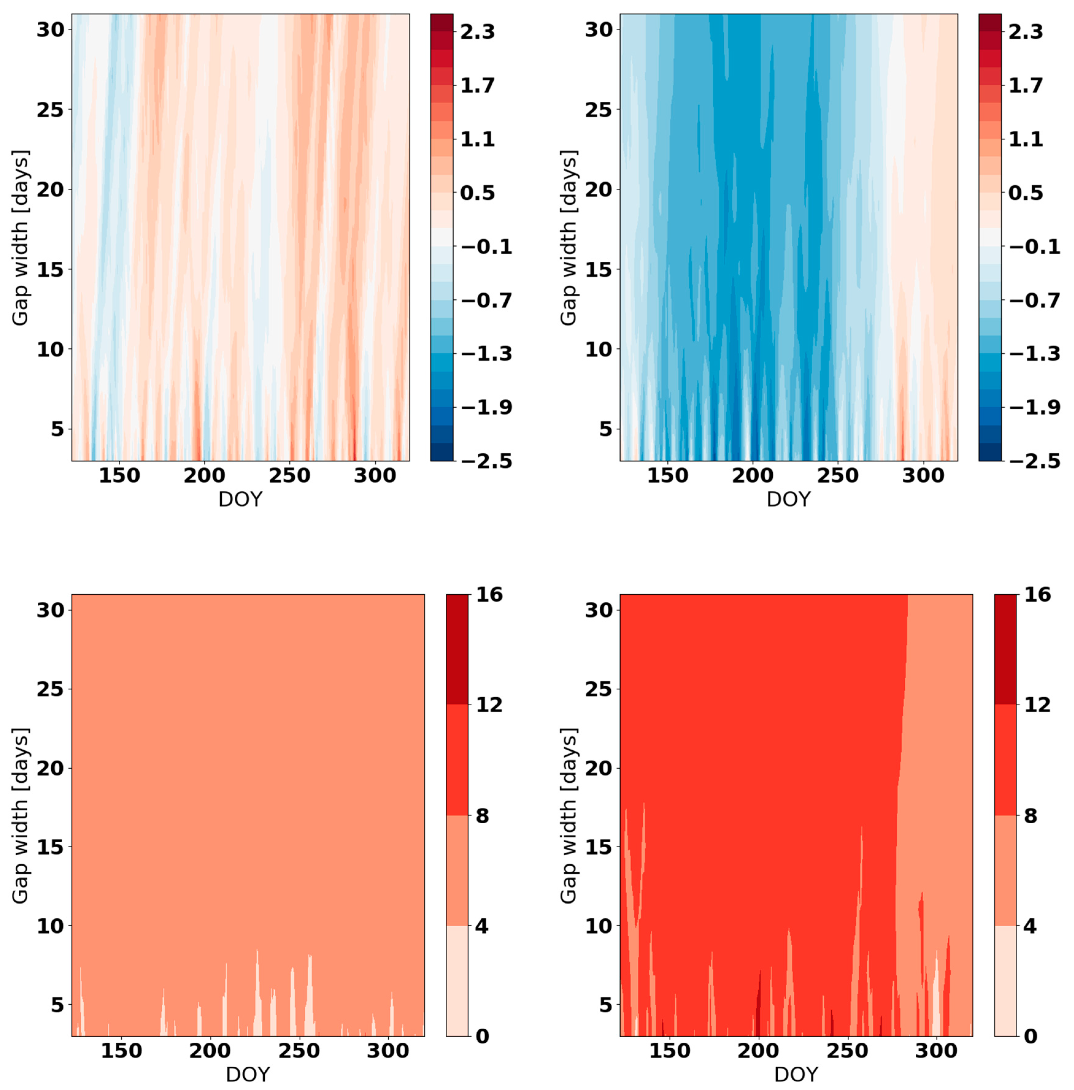
Figure A2.
BDEB (top, left panel), BERA5 (top, right panel), U(B)DEB (bottom, left panel), and U(B)ERA5 (bottom, right panel) calculated using data for DOY 121–334 2017 in Gumpenstein.
Figure A2.
BDEB (top, left panel), BERA5 (top, right panel), U(B)DEB (bottom, left panel), and U(B)ERA5 (bottom, right panel) calculated using data for DOY 121–334 2017 in Gumpenstein.

Figure A3.
BDEB (top, left panel), BERA5 (top, right panel), U(B)DEB (bottom, left panel), and U(B)ERA5 (bottom, right panel) calculated using data for DOY 121–334 2017 in Bahariya.
Figure A3.
BDEB (top, left panel), BERA5 (top, right panel), U(B)DEB (bottom, left panel), and U(B)ERA5 (bottom, right panel) calculated using data for DOY 121–334 2017 in Bahariya.

Figure A4.
BDEB (top, left panel), BERA5 (top, right panel), U(B)DEB (bottom, left panel), and U(B)ERA5 (bottom, right panel) calculated using data for DOY 122–320 2016 in Montecristo.
Figure A4.
BDEB (top, left panel), BERA5 (top, right panel), U(B)DEB (bottom, left panel), and U(B)ERA5 (bottom, right panel) calculated using data for DOY 122–320 2016 in Montecristo.


Figure A5.
BDEB (top, left panel), BERA5 (top, right panel), U(B)DEB (bottom, left panel), and U(B)ERA5 (bottom, right panel) calculated using data for DOY 122–320 2016 in Pianosa.
Figure A5.
BDEB (top, left panel), BERA5 (top, right panel), U(B)DEB (bottom, left panel), and U(B)ERA5 (bottom, right panel) calculated using data for DOY 122–320 2016 in Pianosa.

Appendix C
Figure A6.
RMSEDEB (left panel) and (RMSEDEB-RMSEERA5) difference (right panel) calculated using daily data for DOY 60-273 2014 in Kikinda.
Figure A6.
RMSEDEB (left panel) and (RMSEDEB-RMSEERA5) difference (right panel) calculated using daily data for DOY 60-273 2014 in Kikinda.

Figure A7.
RMSEDEB (left panel) and (RMSEDEB-RMSEERA5) difference (right panel) calculated using daily data for DOY 121–334 2017 in Gumpenstein.
Figure A7.
RMSEDEB (left panel) and (RMSEDEB-RMSEERA5) difference (right panel) calculated using daily data for DOY 121–334 2017 in Gumpenstein.

Figure A8.
RMSEDEB (left panel) and (RMSEDEB-RMSEERA5) difference (right panel) calculated using daily data calculated using daily data for DOY 121–334 2017 in Bahariya.
Figure A8.
RMSEDEB (left panel) and (RMSEDEB-RMSEERA5) difference (right panel) calculated using daily data calculated using daily data for DOY 121–334 2017 in Bahariya.

Figure A9.
RMSEDEB (left panel) and (RMSEDEB-RMSEERA5) difference (right panel) calculated using daily data for DOY 122-320 2016 in Montecristo.
Figure A9.
RMSEDEB (left panel) and (RMSEDEB-RMSEERA5) difference (right panel) calculated using daily data for DOY 122-320 2016 in Montecristo.

Figure A10.
RMSEDEB (left panel) and (RMSEDEB-RMSEERA5) difference (right panel) calculated using daily data for DOY 122-320 2016 in Pianosa.
Figure A10.
RMSEDEB (left panel) and (RMSEDEB-RMSEERA5) difference (right panel) calculated using daily data for DOY 122-320 2016 in Pianosa.

References
- Eischeid, J.K.; Pasteris, P.A.; Diaz, H.F.; Plantico, M.S.; Lott, N.J. Creating a serially complete, national daily time series of temperature and precipitation for the western United States. J. Appl. Meteorol. 2000, 39, 1580–1591. [Google Scholar] [CrossRef]
- Henn, B.; Raleigh, M.S.; Fisher, A.; Lundquist, J.D. A comparison of methods for filling gaps in hourly near-surface air temperature data. J. Hydrometeorol. 2013, 14, 929–945. [Google Scholar] [CrossRef]
- Vuichard, N.; Papale, D. Filling the gaps in meteorological continuous data measured at FLUXNET sites with ERA-Interim reanalysis. Earth Syst. Sci. Data 2015, 7, 157–171. [Google Scholar] [CrossRef] [Green Version]
- Daly, S.F.; Davis, R.; Ochs, E.; Pangburn, T. An approach to spatially distributed snow modelling of the Sacramento and San Joaquin basins, California. Hydrol. Process. 2000, 14, 3257–3271. [Google Scholar] [CrossRef]
- Daly, C.; Gibson, W.P.; Taylor, G.H.; Johnson, G.L.; Pasteris, P. A knowledge-based approach to the statistical mapping of climate. Clim. Res. 2002, 22, 99–113. [Google Scholar] [CrossRef] [Green Version]
- Tobin, C.; Nicotina, L.; Parlange, M.B.; Berne, A.; Rinaldo, A. Improved interpolation of meteorological forcings for hydrologic applications in a Swiss Alpine region. J. Hydrol. 2011, 401, 77–89. [Google Scholar] [CrossRef]
- Garen, D.C.; Johnson, G.L.; Hanson, C.L. Mean Areal Precipitation for daily hydrologic modeling in mountainous regions. JAWRA J. Am. Water Resour. Assoc. 1994, 30, 481–491. [Google Scholar] [CrossRef]
- Hartkamp, A.D.; De Beurs, K.; Stein, A.; White, J.W. Interpolation Techniques for Climate Variables; Cimmyt: Mexico City, Mexico, 1999. [Google Scholar]
- Stahl, K.; Moore, R.D.; Floyer, J.A.; Asplin, M.G.; McKendry, I.G. Comparison of approaches for spatial interpolation of daily air temperature in a large region with complex topography and highly variable station density. Agric. For. Meteorol. 2006, 139, 224–236. [Google Scholar] [CrossRef]
- Pape, R.; Wundram, D.; Löffler, J. Modelling near-surface temperature conditions in high mountain environments: An appraisal. Clim. Res. 2009, 39, 99–109. [Google Scholar] [CrossRef]
- Minder, J.R.; Mote, P.W.; Lundquist, J.D. Surface temperature lapse rates over complex terrain: Lessons from the Cascade Mountains. J. Geophys. Res. Atmos. 2010, 115. [Google Scholar] [CrossRef] [Green Version]
- Rolland, C. Spatial and seasonal variations of air temperature lapse rates in Alpine regions. J. Clim. 2003, 16, 1032–1046. [Google Scholar] [CrossRef]
- Dodson, R.; Marks, D. Daily air temperature interpolated at high spatial resolution over a large mountainous region. Clim. Res. 1997, 8, 1–20. [Google Scholar] [CrossRef] [Green Version]
- Claridge, D.E.; Chen, H. Missing data estimation for 1–6 h gaps in energy use and weather data using different statistical methods. Int. J. Energy Res. 2006, 30, 1075–1091. [Google Scholar] [CrossRef]
- Liston, G.E.; Elder, K. A meteorological distribution system for high-resolution terrestrial modeling (MicroMet). J. Hydrometeorol. 2006, 7, 217–234. [Google Scholar] [CrossRef]
- Von Storch, H.; Zwiers, F.W.; Livezey, R.E. Statistical analysis in climate research. Nature 2000, 404, 544. [Google Scholar]
- Beckers, J.-M.; Rixen, M. EOF calculations and data filling from incomplete oceanographic datasets. J. Atmos. Ocean. Technol. 2003, 20, 1839–1856. [Google Scholar] [CrossRef]
- Blyth, E.; Gash, J.; Lloyd, A.; Pryor, M.; Weedon, G.P.; Shuttleworth, J. Evaluating the JULES land surface model energy fluxes using FLUXNET data. J. Hydrometeorol. 2010, 11, 509–519. [Google Scholar] [CrossRef]
- Stöckli, R.; Lawrence, D.M.; Niu, G.-Y.; Oleson, K.W.; Thornton, P.E.; Yang, Z.-L.; Bonan, G.B.; Denning, A.S.; Running, S.W. Use of FLUXNET in the Community Land Model development. J. Geophys. Res. Biogeosci. 2008, 113. [Google Scholar] [CrossRef] [Green Version]
- Papale, D. Data gap filling. In Eddy Covariance; Springer: Berlin, Germany, 2012; pp. 159–172. [Google Scholar]
- Puri, K. Numerical weather prediction in the tropics. J. Meteorol. Soc. Jpn. Ser II 1986, 64, 605–631. [Google Scholar] [CrossRef]
- Sandu, I.; Bechtold, P.; Beljaars, A.; Bozzo, A.; Pithan, F.; Shepherd, T.G.; Zadra, A. Impacts of parameterized orographic drag on the Northern Hemisphere winter circulation. J. Adv. Model. Earth Syst. 2016, 8, 196–211. [Google Scholar] [CrossRef] [Green Version]
- Haiden, T.; Sandu, I.; Balsamo, G.; Arduini, G.; Beljaar, A. Addressing Biases in Near-Surface Forecasts; ECMWF Newsletter; European Centre for Medium-Range Weather Forecasts: Shinfield Park, Reading, UK, 2018; p. 157. [Google Scholar]
- Lim, Y.-K.; Cai, M.; Kalnay, E.; Zhou, L. Observational evidence of sensitivity of surface climate changes to land types and urbanization. Geophys. Res. Lett. 2005, 32. [Google Scholar] [CrossRef] [Green Version]
- ERA5 Data Documentation—Copernicus Knowledge Base—ECMWF Confluence Wiki. Available online: https://confluence.ecmwf.int//display/CKB/ERA5+data+documentation (accessed on 5 November 2018).
- LaMMA Consortium. Available online: http://www.lamma.rete.toscana.it/ (accessed on 24 November 2018).
- Raible, C.C.; Bischof, G.; Fraedrich, K.; Kirk, E. Statistical single-station short-term forecasting of temperature and probability of precipitation: Area interpolation and NWP combination. Weather Forecast. 1999, 14, 203–214. [Google Scholar] [CrossRef]
- FDA U. NIST: Multi-Agency Radiological Laboratory Analytical Protocols Manual (MARLAP); FDA, USGS, NUREG-1576. EPA 402-B-04-001C, NTIS PB2004-105421; FDA: Alexandria, VA, USA, 2004. [Google Scholar]
- D’Agostino, R.B. An omnibus test of normality for moderate and large size samples. Biometrika 1971, 58, 341–348. [Google Scholar] [CrossRef]
- D’Agostino, R.B.; Pearson, E.S. Tests for departure from normality. Empirical results for the distributions of b 2 and√ b. Biometrika 1973, 60, 613–622. [Google Scholar] [CrossRef]
- Pavlovič, F.; Nastran, J.; Nedeljković, D. Determining the 95% Confidence Interval of Arbitrary Non-Gaussian probability distributions. Available online: http://www.imeko2009.it.pt/Papers/FP_81.pdf (accessed on 13 October 2018).
- Dumas, M.D. Changes in temperature and temperature gradients in the French Northern Alps during the last century. Theor. Appl. Climatol. 2013, 111, 223–233. [Google Scholar] [CrossRef]
- Evans, J.D. Straightforward Statistics for the Behavioral Sciences; Brooks/Cole Publishing Company: Pacific Grove, CA, USA, 1996; ISBN 978-0-534-23100-2. [Google Scholar]
- Cao, H.X.; Mitchell, J.F.B.; Lavery, J.R. Simulated Diurnal Range and Variability of Surface Temperature in a Global Climate Model for Present and Doubled CO2 Climates. J. Clim. 1992, 5, 920–943. [Google Scholar] [CrossRef]
- Decker, M.; Brunke, M.A.; Wang, Z.; Sakaguchi, K.; Zeng, X.; Bosilovich, M.G. Evaluation of the reanalysis products from GSFC, NCEP, and ECMWF using flux tower observations. J. Clim. 2012, 25, 1916–1944. [Google Scholar] [CrossRef]
- Chen, Z. A Serially Complete, U.S. Dataset of Temperature and Precipitation for Decision Support Systems. J. Environ. Inform. 2006, 8, 86–99. [Google Scholar] [CrossRef]
Figure 1.
Altitude (m a.s.l.) and position of the Kikinda (Serbia) automated weather station (AWS).

Figure 2.
Altitude (m a.s.l.) and position of the Gumpenstein (Austria) automated weather station (AWS).
Figure 2.
Altitude (m a.s.l.) and position of the Gumpenstein (Austria) automated weather station (AWS).

Figure 3.
Altitude (m a.s.l.) and position of the el-Bahariya oasis (Egypt) automated weather station (AWS).
Figure 3.
Altitude (m a.s.l.) and position of the el-Bahariya oasis (Egypt) automated weather station (AWS).

Figure 4.
Altitude (m a.s.l.) and position of the Montecristo Island (Italy) automated weather station (AWS).
Figure 4.
Altitude (m a.s.l.) and position of the Montecristo Island (Italy) automated weather station (AWS).

Figure 5.
Altitude (m a.s.l.) and position of the Pianosa Island (Italy) automated weather station (AWS).
Figure 5.
Altitude (m a.s.l.) and position of the Pianosa Island (Italy) automated weather station (AWS).

Figure 6.
(a) Time series with a gap in temperature observations. The blue line represents observations, the dashed blue line represents hidden observations, the red line represents ERA5 values for the nearest grid point, and the green line represents the result of the debiasing process; (b) Linear regression of learning data for one-time step in the gap following the standard equation: .

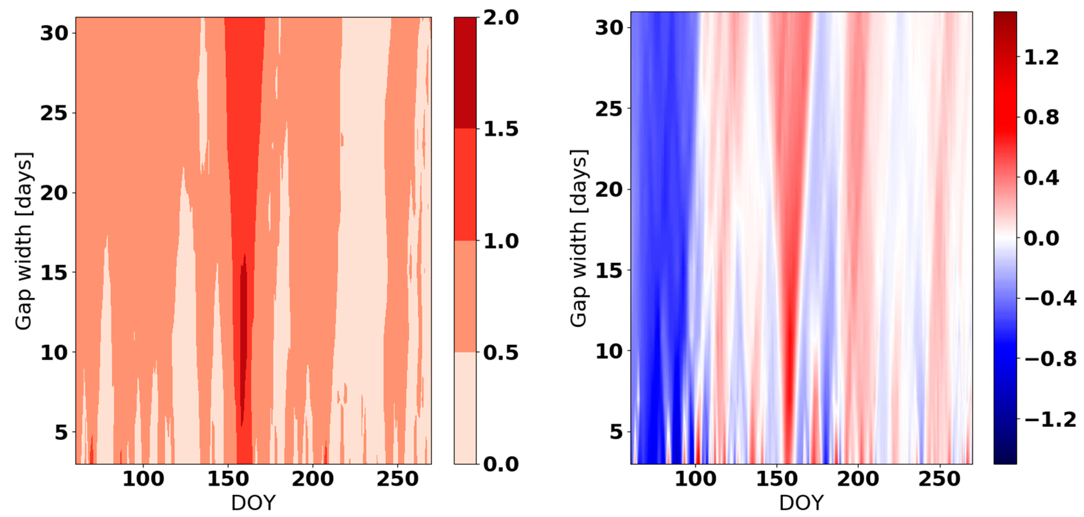
Figure 7.
RMSEDEB (left panel) and (RMSEDEB-RMSEERA5) difference (right panel) for DOY 60–273 in 2014 in Kikinda (Serbia).
Figure 7.
RMSEDEB (left panel) and (RMSEDEB-RMSEERA5) difference (right panel) for DOY 60–273 in 2014 in Kikinda (Serbia).

Figure 8.
Standard deviation of the observed data which are used for bias correction for DOY 60–273 in 2014 in Kikinda (Serbia).
Figure 8.
Standard deviation of the observed data which are used for bias correction for DOY 60–273 in 2014 in Kikinda (Serbia).

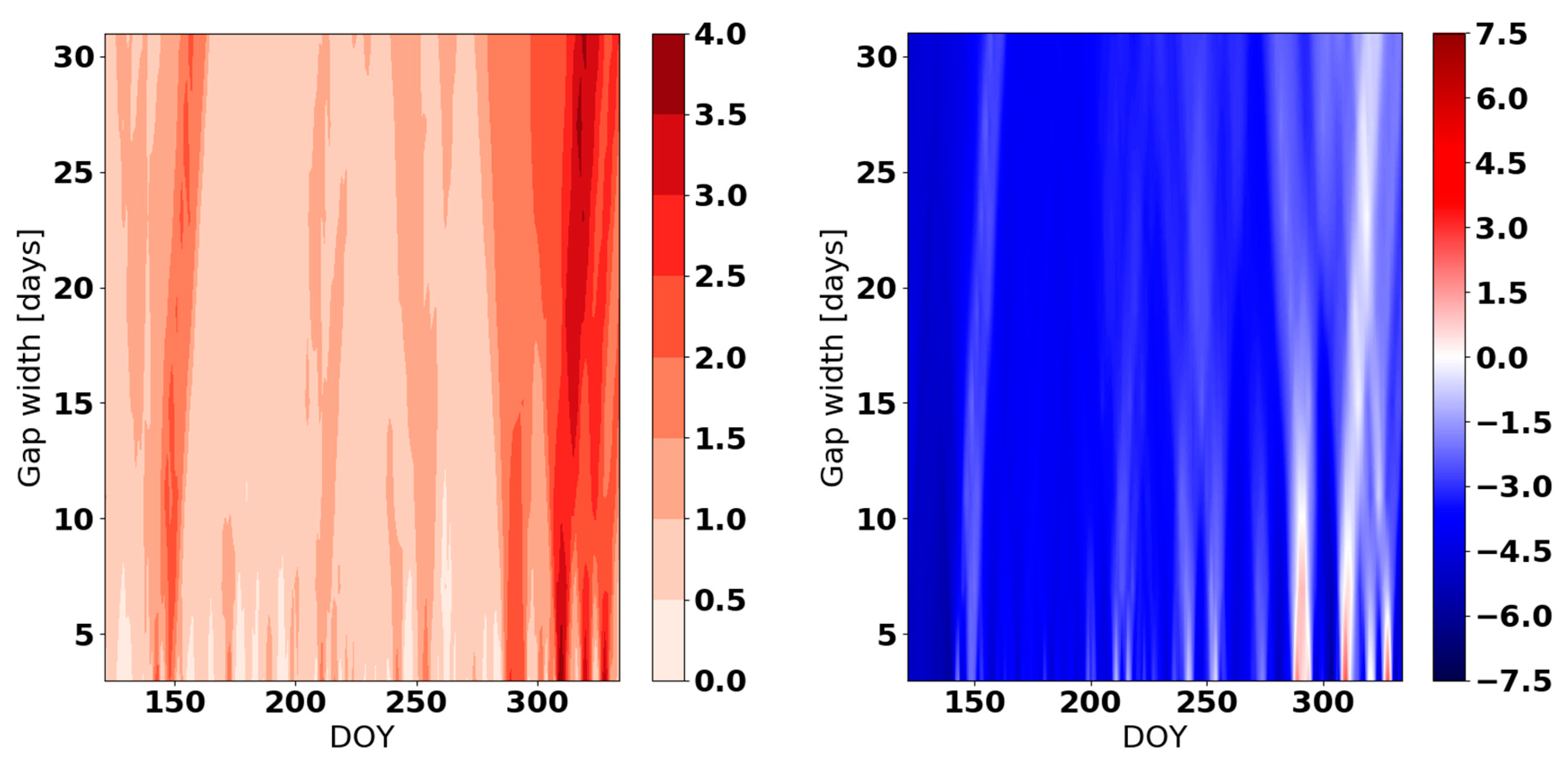
Figure 9.
RMSEDEB (left panel) and (RMSEDEB-RMSEERA5) difference (right panel) for DOY 121–334 in 2017 in Gumpenstein (Austria).
Figure 9.
RMSEDEB (left panel) and (RMSEDEB-RMSEERA5) difference (right panel) for DOY 121–334 in 2017 in Gumpenstein (Austria).

Figure 10.
Standard deviation of observed data which were used for bias correction for DOY 121–334 in 2017 in Gumpenstein (Austria).
Figure 10.
Standard deviation of observed data which were used for bias correction for DOY 121–334 in 2017 in Gumpenstein (Austria).

Figure 11.
RMSEDEB (left panel) and (RMSEDEB-RMSEERA5) difference (right panel) for DOY 121–334 in 2017 in Bahariya (Egypt).
Figure 11.
RMSEDEB (left panel) and (RMSEDEB-RMSEERA5) difference (right panel) for DOY 121–334 in 2017 in Bahariya (Egypt).

Figure 12.
Standard deviation of observed data which are used for bias correction for DOY 121–334 in 2017 in Bahariya (Egypt).
Figure 12.
Standard deviation of observed data which are used for bias correction for DOY 121–334 in 2017 in Bahariya (Egypt).

Figure 13.
Daily variation in air temperature for DOY 215–226 inBahariya (Egypt).

Figure 14.
Standard deviation of the observed data which were used for bias correction for the islands of Montecristo (left panel) and Pianosa (right panel) for the DOY 122–320 in 2016.
Figure 14.
Standard deviation of the observed data which were used for bias correction for the islands of Montecristo (left panel) and Pianosa (right panel) for the DOY 122–320 in 2016.

Figure 15.
RMSEDEB (left panel) and (RMSEDEB-RMSEERA5) difference (right panel) for DOY 122–320in 2016 in Montecristo Island (Italy).
Figure 15.
RMSEDEB (left panel) and (RMSEDEB-RMSEERA5) difference (right panel) for DOY 122–320in 2016 in Montecristo Island (Italy).

Figure 16.
RMSEDEB (left panel) and (RMSEDEB-RMSEERA5) difference (right panel) for DOY 122–320 in 2016 in Pianosa Island (Italy).
Figure 16.
RMSEDEB (left panel) and (RMSEDEB-RMSEERA5) difference (right panel) for DOY 122–320 in 2016 in Pianosa Island (Italy).

Figure 17.
RMSEDEB for gap width = 1 and the correlation coefficient between the standard deviation of the observed data used for linear regression and RMSEDEB for Kikinda (Serbia; top left), Bahariya (Egypt; top right), Gumpenstein (Austria; middle), Montecristo (Italy; bottom left) and Pianosa (Italy; bottom right).


Table 1.
Locations used in the study (* see surface on ERA5).
| Location | Time Series | Landscape | Position | ERA5 | ||||
|---|---|---|---|---|---|---|---|---|
| Latitude (°) | Longitude (°) | Altitude (m) | Latitude (°) | Longitude (°) | Altitude (m) | |||
| Kikinda | 2014–2017 | Lowland | 45.87 | 20.46 | 82 | 45.9 | 20.4 | 75 |
| Gumpenstein | 2014–2017 | Mountains | 47.49 | 14.09 | 700 | 47.4 | 14.1 | 1080 |
| Bahariya | 2017 | Desert | 28.41 | 28.93 | 99 | 28.4 | 28.9 | 97 |
| Montecristo | 2016 | Island | 42.34 | 10.31 | 645 | 42.3 | 10.2 | * |
| Pianosa | 2016 | Island | 42.58 | 10.08 | 29 | 42.6 | 10.2 | * |
Table 2.
Mean bias, mean bias uncertainty, and mean RMSE for all gap widths in selected locations.
| Mean B | Mean U(B) | Mean RMSE | ||||
|---|---|---|---|---|---|---|
| ERA5 | DEB | ERA5 | DEB | ERA5 | DEB | |
| Kikinda | 0.387 | −0.027 | 6.56 | 5.61 | 1.563 | 1.321 |
| Bahariya | −0.723 | −0.033 | 8.39 | 6.67 | 2.046 | 1.536 |
| Gumpenstein | −4.385 | 0.556 | 10.18 | 7.37 | 4.969 | 1.877 |
| Montecristo | −0.009 | 0.284 | 5.58 | 4.27 | 1.367 | 1.079 |
| Pianosa | −0.769 | 0.222 | 8.69 | 5.32 | 2.158 | 1.260 |
Table 3.
Maximum absolute values of (RMSEDEB-RMSEERA5) difference and RMSEDEB calculated using hourly and daily data for gap filling.
Table 3.
Maximum absolute values of (RMSEDEB-RMSEERA5) difference and RMSEDEB calculated using hourly and daily data for gap filling.
| Location | Bahariya (°C) | Gumpenstein (°C) | Kikinda (°C) | Montecristo (°C) | Pianosa (°C) |
|---|---|---|---|---|---|
| max(|RMSEDEB-RMSEERA5|) for hourly data | 1.81 | 6.34 | 0.87 | 0.95 | 2.12 |
| max(|RMSEDEB-RMSEERA5|) for daily average | 1.31 | 7.32 | 1.03 | 1.08 | 1.63 |
| max(|RMSEDEB|) for hourly data | 2.54 | 4.19 | 2.21 | 2.18 | 2.31 |
| max(|RMSEDEB|) for daily average | 1.82 | 4.02 | 1.69 | 2.06 | 1.98 |
© 2019 by the authors. Licensee MDPI, Basel, Switzerland. This article is an open access article distributed under the terms and conditions of the Creative Commons Attribution (CC BY) license (http://creativecommons.org/licenses/by/4.0/).
Share and Cite
MDPI and ACS Style
Lompar, M.; Lalić, B.; Dekić, L.; Petrić, M. Filling Gaps in Hourly Air Temperature Data Using Debiased ERA5 Data. Atmosphere 2019, 10, 13. https://doi.org/10.3390/atmos10010013
AMA Style
Lompar M, Lalić B, Dekić L, Petrić M. Filling Gaps in Hourly Air Temperature Data Using Debiased ERA5 Data. Atmosphere. 2019; 10(1):13. https://doi.org/10.3390/atmos10010013
Chicago/Turabian StyleLompar, Miloš, Branislava Lalić, Ljiljana Dekić, and Mina Petrić. 2019. "Filling Gaps in Hourly Air Temperature Data Using Debiased ERA5 Data" Atmosphere 10, no. 1: 13. https://doi.org/10.3390/atmos10010013
Note that from the first issue of 2016, this journal uses article numbers instead of page numbers. See further details here.