Ensemble Sensitivity Analysis-Based Ensemble Transform with 3D Rescaling Initialization Method for Storm-Scale Ensemble Forecast

Key Laboratory of Meteorological Disaster of Ministry of Education/Collaborative Innovation Center on Forecast and Evaluation of Meteorological Disasters, Nanjing University of Information Science & Technology, Nanjing 210044, China
*
Author to whom correspondence should be addressed.
Atmosphere 2019, 10(1), 24; https://doi.org/10.3390/atmos10010024
Submission received: 8 December 2018
/
Revised: 26 December 2018
/
Accepted: 8 January 2019
/
Published: 10 January 2019
(This article belongs to the Special Issue Advancements in Mesoscale Weather Analysis and Prediction)
Abstract
:In order to further investigate the influence of ensemble generation methods on the storm-scale ensemble forecast (SSEF) system, a new ensemble sensitivity analysis-based ensemble transform with 3D rescaling (ET_3DR_ESA) method was developed. The Weather Research and Forecasting (WRF) Model was used to numerically simulate a squall line that occurred in the Jianghuai region in China on 12 July 2014. In this study, initial perturbations were generated via ET_3DR_ESA, and the ensemble forecast performance was compared to that of the dynamical downscaling (Down) method and the ensemble transform with 3D rescaling (ET_3DR) method. Results from a set of experiments indicate that ET_3DR_ESA linked to multi-scale environmental fields generates initial perturbations that can not only capture analysis uncertainties, but also match the actual synoptic conditions. Such perturbations produce faster ensemble spread growth, lower root-mean-square error, and a lower percentage of outliers, especially during the peak period of the squall line. In addition, ET_3DR_ESA can effectively reduce the energy dissipation on different scales through the analysis of the power spectrum. Moreover, the intensity and distribution forecasts of heavy rainfall from the ET_3DR_ESA ensemble forecast system were demonstrated to better match the observation. Furthermore, according to results of the relative operating characteristic (ROC) test, Brier score (BS), and equitable threat score (ETS), ET_3DR_ESA significantly improved the forecast skills for heavy rain (15–30 mm/12 h) and extreme rain (>30 mm/12 h), which are critical to the realization of accurate storm-scale system precipitation forecasts. In general, these results suggest that ET_3DR_ESA can be effectively applied to SSEF systems.
1. Introduction
Ensemble forecasting, which is an effective method to estimate forecast uncertainties, can achieve higher numerical forecast skill than deterministic forecasts [1]. To date, global medium-range ensemble forecast (forecast time: 3–15 d, horizontal resolution: 30–100 km) [2,3] and regional short-range ensemble forecast techniques (forecast time: 1–3 d, horizontal resolution: 10–20 km) [4] have been relatively effective. However, because of the short life history, small spatial scale, and complex three-dimensional structure of storm-scale systems [5], their error growth mode is quite different from that of large-scale and meso-scale systems. Therefore, the development of a reasonable and effective storm-scale ensemble forecast (SSEF) system (forecast time: less than 1 d, horizontal resolution: 1–4 km) [6,7] is particularly critical, and has become a research focus for international numerical weather prediction centers.
Ensemble generation methods seek to create a set of initial perturbations that can represent analysis errors in a numerical weather prediction system in order to improve its probabilistic forecast performance [8]. A reasonable ensemble generation method is the foundation of SSEF systems. Accurately representing analysis uncertainties, adapting to model resolutions and regions, and matching the lateral boundary perturbations are three basic conditions for initial perturbations in regional and SSEF systems [4].
Dynamical downscaling (Down) [9] is a common ensemble generation method that directly interpolates global ensemble forecast perturbations into the grid domain of an SSEF system to generate initial perturbations. This method has been proven to effectively minimize computational resources and match lateral boundary perturbations. However, it is unable to obtain small-scale perturbations, which are essential for storm-scale systems [10]. The ensemble transform with rescaling (ETR) method has been proven to be an effective global ensemble generation method in the National Centers for Environmental Prediction (NCEP) global forecast system [11]. This method entails transforming forecast perturbations into analysis perturbations via an ensemble transformation matrix, and then imposing a regional rescaling process.
Ma et al. [8] defined the rescaling factor as the ratio of the mask to the square root of the kinetic energy norm of analysis perturbations at each grid point in NCEP’s operational ETR. The mask was calculated based on the long-term-averaged root-mean-square of the analysis error variance in the kinetic energy norm at the 500 hPa level. However, the two-dimensional mask was found to have the following three problems: (1) It is unable to represent the vertical structure of analysis uncertainties, (2) it is unable to update the mask with the real-time data assimilation system, and (3) it is more reasonable to use the total energy norm than the kinetic energy norm.
Thus, an ensemble generation method, the ensemble transform with 3D rescaling (ET_3DR) method, was introduced with a new mask that uses the total energy norm obtained from the 80-member ensemble analysis generated by the NCEP’s hybrid 3D-Var/EnKF system [12]. Results from experiments revealed that the ensemble spread of ET_3DR grew faster, and that the ET_3DR forecast outperformed that of the ETR. Alternatively, in contrast to Down, the initial perturbations generated by ET_3DR contain analysis uncertainties, and are in agreement with the model resolutions. This implies that applying ET_3DR to SSEF systems makes sense.
Considering the differences between storm-scale systems and synoptic systems, it is particularly important to establish the statistical relationship between convective forecasts and the previous environmental fields to find the more sensitive factors [13]. Torn et al. [14] proposed an ensemble sensitivity analysis (ESA) method, which can quickly and strictly estimate the linear relationship between forecast variables and the initial conditions by using ensemble statistics. ESA can intuitively reflect the growth features of the ensemble initial perturbations in the model and the influence of the synoptic-scale environmental field on the model forecast. To date, ESA has been widely used to analyze synoptic-scale systems, such as extratropical cyclones [14,15,16] and tropical cyclones [17,18,19,20]. In recent years, the utility of ESA has been investigated on the meso-scale [21,22,23]. Wile et al. [24] developed an ESA-based technique to directly control ensemble initial perturbations. Such perturbations can effectively match the synoptic conditions and link to the environmental field, thereby verifying the ability of ESA to identify sensitive factors.
Because SSEF systems are necessary to realize accurate severe convection forecasts, further research and the development of SSEF-based effective ensemble generation methods are essential. As mentioned above, ET_3DR can effectively increase the accuracy of global ensemble forecasts. However, it is not suitable for SSEF systems. Alternatively, perturbations controlled via ESA have been proven to better match the synoptic conditions. Therefore, it is possible to implement ESA within ET_3DR; this technique is hereafter referred to as ET_3DR_ESA. In order to investigate the error growth modes of ET_EDR_ESA-generated initial perturbations and the resulting impact on ensemble forecasts, we performed a set of experiments on a squall line that occurred in the Jianghuai region of China by using the Weather Research and Forecasting (WRF) model to compare the results of Down, ET_3DR, and ET_3DR_ESA.
2. Data and Methods
2.1. Experimental Design
A squall line occurred in the Jianghuai region of China from 0300 UTC to 1200 UTC on 12 July 2014, and reached its peak in southern Anhui at 0800 UTC, with a maximum radar reflectivity of 55 dBZ. Up until 1200 UTC, the squall line convection zone weakened to form stratiform clouds. The movement of the precipitation zone corresponded well with that of the squall line convection system. The 12-h accumulated precipitation that was present from 0000 UTC to 1200 UTC was mainly distributed from east to west, and the precipitation center located in southern Anhui and southern Jiangsu reported the maximum precipitation to be close to 70 mm.
We performed three experiments (Table 1) to evaluate the impact of ET_3DR_ESA on a SSEF system, and its advantages over Down and ET_3DR. In this study, Down was purposed to directly interpolate the NCEP global ensemble forecast perturbations into the inner domain as initial perturbations. In addition, in order to qualitatively compare the three methods, perturbations were only added to the inner domain; thus, lateral boundary and model perturbations were not introduced into the experiments.
In each experiment, the WRF model (WRF 3.9.1.1) was applied to data spanning 0000 UTC through 1200 UTC on 12 July 2014. The nested model domain had 34 levels in the vertical direction. The inner domain (i.e., the analysis domain) had 4-km horizontal grid spacing and 168 × 168 grid points, covering the entire Jianghuai region (see Figure 2); the outer domain was assigned 12-km horizontal grid spacing and 160 × 160 grid points. Moreover, the following physical parameterizations were applied: the WSM5 microphysical scheme [25], the YSU PBL physics scheme [26], the RRTM longwave radiation scheme [27], the Dudhia shortwave radiation scheme [28], and the Kain-Fritsch cumulus parameterization scheme [29] (only used in the outer domain).
The initial and lateral boundary conditions were determined based on the global 1° × 1° NCEP FNL reanalysis data, with NCEP 20-member global 0.5° × 0.5° ensemble forecast data implemented as the initial perturbations of the inner domain for each experiment. NCEP operational 80-member hybrid 3D-Var/EnKF data assimilation system data were used to update perturbations in ET_3DR and ET_3DR_ESA. In addition, the hourly 0.1° × 0.1° real-time precipitation blending data from the National Meteorological Information Center (China) were employed as the observed precipitation data.
2.2. ET_3DR_ESA Method
In the ET_3DR scheme [8], the analysis perturbations matrix is generated from the forecast perturbations matrix via a transformation matrix , as follows:
As shown in Wei et al. [11], the transformation matrix is calculated as follows:
matrix contains the orthonormal eigenvectors of the matrix , and matrix contains the corresponding eigenvalues, where n represents the ensemble size. From Wei et al. [11], we know that the first eigenvalues are nonzero, whereas the last eigenvalue is zero, and its associated eigenvector is a constant. Thus, a diagonal matrix Ғ is defined by setting the last eigenvalue in to equal a nonzero constant α. The diagonal matrix contains the analysis error variances.
After the transformation, all perturbations are orthogonal, but not centered. In order to re-center the initial perturbations around the analysis field to improve the performance of the ensemble mean, we need to perform a simplex transformation with on all analysis perturbations, as follows:
To ensure that the initial spread distribution is similar to the analysis error variance, we impose a regional rescaling process; this means that will be rescaled by using a rescaling factor , which is given as
where pertb is the square root of the total energy norm from , and the mask denotes the root-mean-square of the total energy norm computed from the NCEP operational 80-member hybrid 3D-Var/EnKF data assimilation system. According to Equation (4), the mask will only suppress the amplitude of perturbations, and not increase it.
As discussed in Section 1, in consideration of the complexity of storm-scale systems, ESA is used to establish the statistical relationship between convective forecasts and the environmental fields before convection. Ancell et al. [30] proposed that, for a chosen model forecast variable R, its ensemble sensitivity (ES) to the model state variable x at an earlier time can be defined as
where cov and var denote the covariance and variance of the given variables, respectively, and measure the linear relationship between two variables and the analysis spread of x relative to the ensemble mean.
In this study, we employed ESA to control ET_3DR-generated perturbations in order to obtain the initial perturbations of ET_3DR_ESA. The control process entailed multiplying the analysis perturbations obtained via ET_3DR with the ES (subsequent to passing a 0.05-level significance test) after standardization. A schematic diagram of the ET_3DR_ESA ensemble forecast system is shown in Figure 1. The experiment cycled for three days, from 0000 UTC on 9 July 2014 to 0000 UTC on 12 July 2014, and the perturbation variables and model state variables were selected as temperature T, zonal wind U, radial wind V, and water vapor mixing ratio Q. The perturbations at the initial time were obtained from NCEP 20-member global 0.5° × 0.5° ensemble forecast data, and then implemented in a 6-h forecast simulation for the 20 members to obtain the 9 July 0600 UTC forecast perturbations. The perturbations were subsequently updated every six hours by using ET_3DR_ESA. At 0000 UTC on 12 July 2014, the ultimate analysis perturbations were incorporated into the initial conditions for a 12-h ensemble forecast experiment.
3. Results
3.1. General Nature of Convective Ensemble Sensitivity
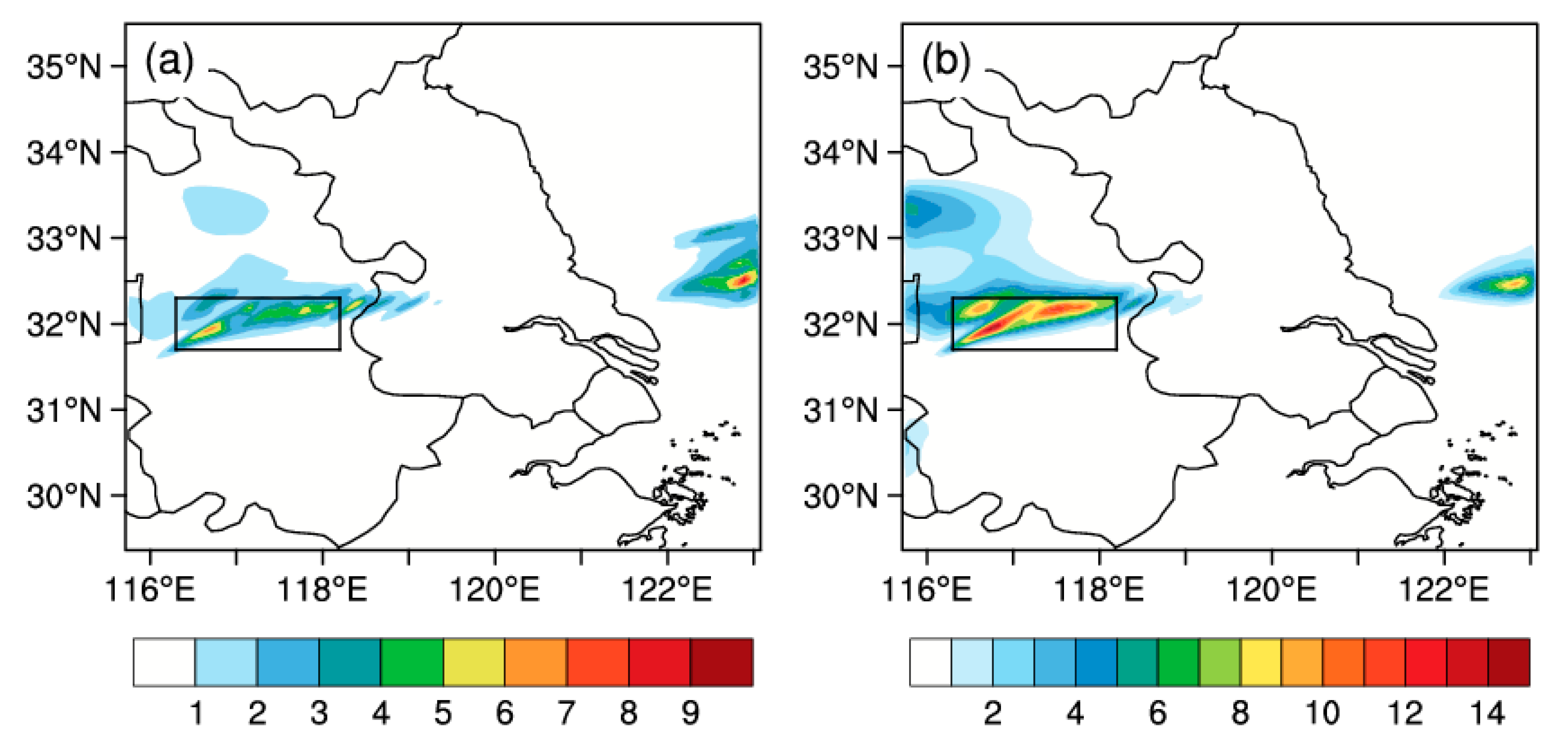
In order to avoid spurious correlations and to accurately reflect the linear relationship between forecast variables and state variables, before the 12-h ensemble forecast, the inspection of ensemble sensitivity was applied to the squall line by using the forecast variable R that was defined as the accumulated precipitation from 0000 UTC to 0300 UTC on 12 July 2014, (i.e., before the squall line occurred) over the response region indicated in Figure 2 by a black rectangle. As shown in Figure 2, most of the heavy precipitation and the majority of the large spread region are located in central Anhui. This shows that there are significant differences between ensemble members in the heavy precipitation region; this information is important in precipitation forecasts.
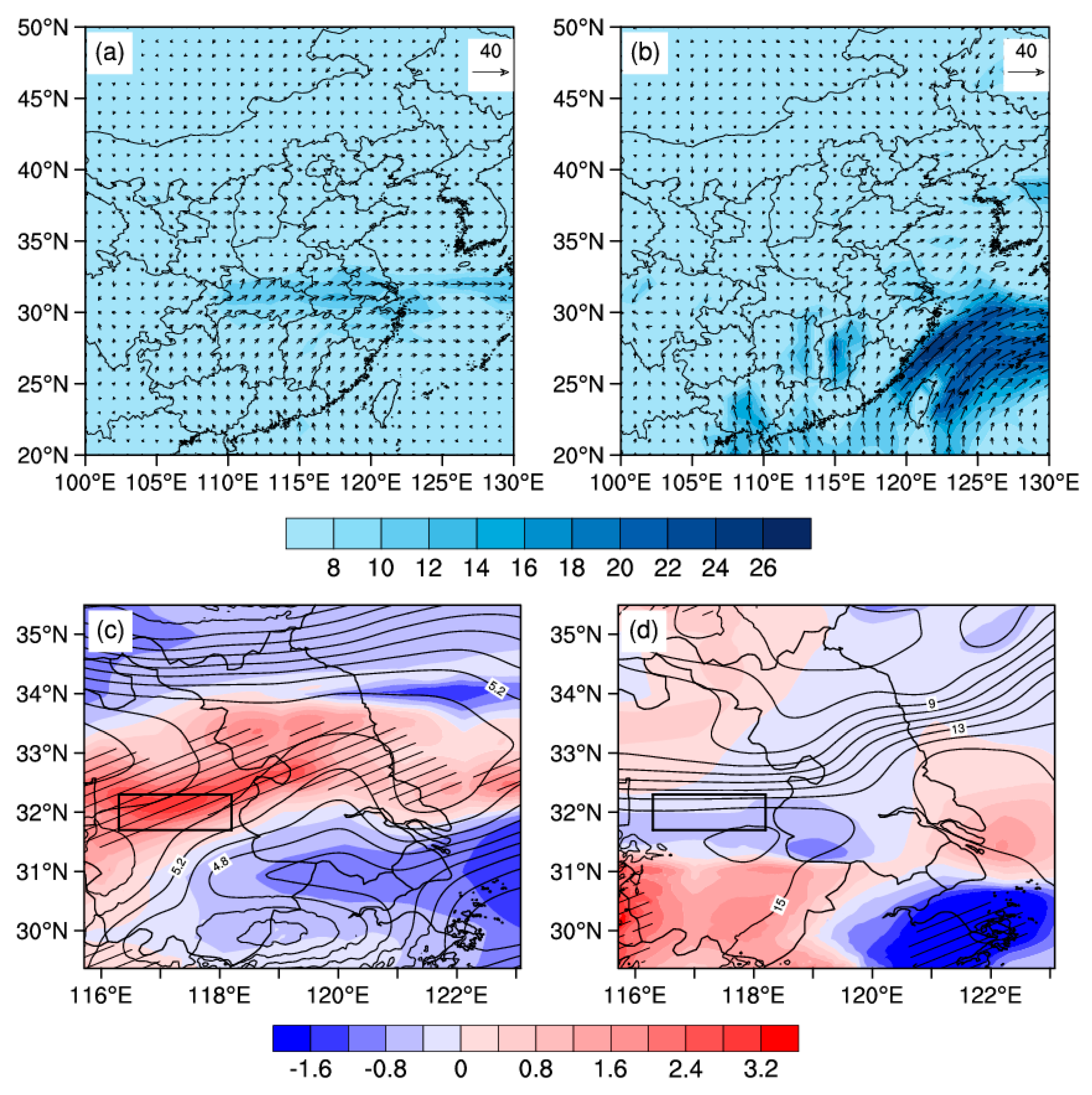
The general nature and reliability of ensemble sensitivity for this squall line process can be analyzed via sensitivity fields and environmental fields. This analysis enables inspection of the thermodynamic sensitivity, which provides information about relatively small-scale features while also maintaining a relationship with the synoptic-scale features [21]. The synoptic-scale circulation patterns are shown in Figure 3a,b. Before the occurrence of the squall line, the Jianghuai region was located to the south of a 200-hPa upper jet stream, and in front of a deep 500-hPa upper trough. Also during this time, the subtropical high shifted to 35 °N, and a large amount of warm-wet air was transported to the Jianghuai region; additionally, there was a strong 850-hPa trough. The wind on the north side of the trough was weak, and that on the south side was strong; these conditions were conducive to the precipitation and accumulation of warm-wet air in the Jianghuai region.
The sensitivity of the forecast variable R to 500-hPa and 850-hPa temperature highlights a number of features (Figure 3c,d). The first is the positive sensitivity in the response region at 500 hPa, which indicates a relatively warmer temperature in this region that is related to more precipitation during this time. Because of the large amount of precipitation in the response region, this feature is interpreted as the relationship between R and the variables that it affects. Another prominent feature is a highly negative sensitivity area over the Jianghuai region at 500 hPa; this area corresponds to the strong cold trough in western Jiangsu and the weak cold trough in southern Jiangsu. This feature suggests that the relatively colder temperature there positively contributes to the precipitation in the response area. The significant positive sensitivity surrounding the response region at 850 hPa indicates that the relatively warmer temperature caused by warm-wet air contributes to precipitation; this feature is identical to that of 850-hPa synoptic-scale circulation patterns.
Abundant moisture is the main source of the convection energy. Water vapor flux can be used to analyze the water vapor transport of strong convections (Figure 4a,b). At 0000 UTC on 12 July 2014, a large water vapor area covered the Jianghuai region at 500 hPa; water vapor in the south was transported to this area under the influence of a southwest air current, which contributed to the precipitation in the Jianghuai region. Considering the sensitivity to moisture (Figure 4c,d), the area of positive sensitivity over the Jianghuai region at 500 hPa is in the same location as negative sensitivity to temperature, which is in the previously mentioned cold air. This feature suggests that colder and wetter air there is related to increased precipitation which is a consequence of the downdraft. At 850 hPa, the significant positive sensitivity region in southwestern Anhui, which corresponds to the large water-vapor flux region in Figure 4b, proves that the southwest warm-wet air current produces more precipitation, as this feature is known to be associated with water vapor flux.
Through the analysis of thermodynamic and moisture sensitivities, it has been found that the features of ESA in finer-scale information and linkages to the synoptic-scale facilitate a better understanding of the sensitivity of a precipitation forecast to the state variables, implying that it is meaningful to apply ESA to control initial perturbations.
3.2. Quantitative Evaluation of the Ensemble Forecasts
In an ideal ensemble forecast system, the relationship between the growth rate of initial perturbations and the forecast error should not change [31]. The ensemble spread, which measures the deviation of ensemble members from the ensemble mean, is the method used to evaluate the growth rate of perturbations.
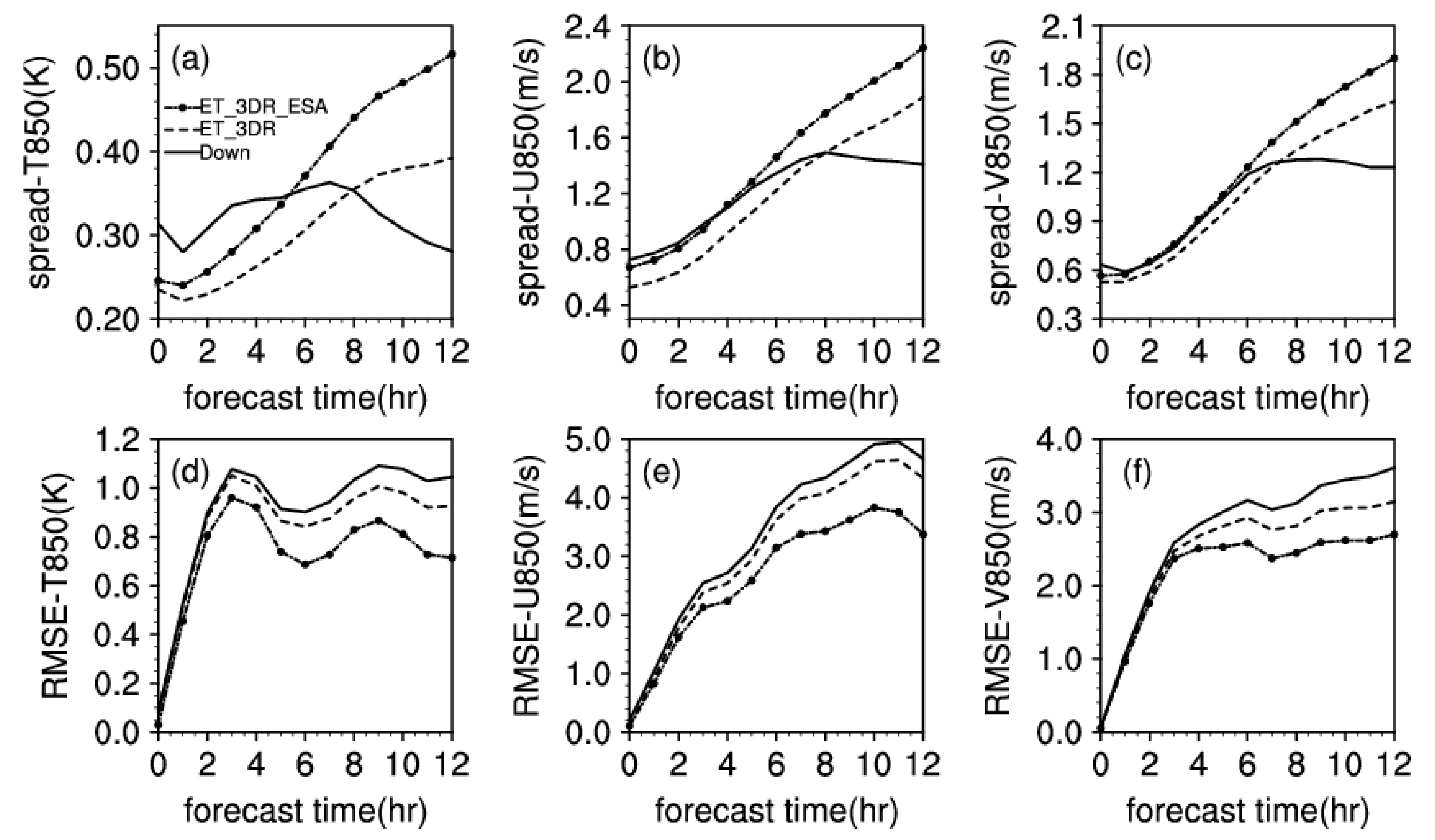
Figure 5a–c shows the 850-hPa T, U, and V ensemble spreads for each of the three representative experiments (Down, ET_3DR, and ET_3DR_ESA). Prior to the occurrence of the squall line (forecast time: 0–3 h), the Down spread containing only large-scale perturbations was larger than that of the other two experiments. However, during the developmental period (forecast time: 4–6 h) and peak period (forecast time: 7–9 h), the ET_3DR_ESA and ET_3DR spreads exceeded the corresponding Down spreads, exhibiting fast growth throughout the forecast time; during these two periods, the corresponding Down spreads began to decrease. In addition, the ET_3DR ESA spread grew faster and covered a larger area than the ET_3DR spread; this was particularly evident during the peak period of the squall line. The superior performance of ET_3DR_ESA is attributed to the multi-scale interaction in ESA that enables a more accurate reflection of the growth of initial errors.
The ensemble spread is merely a statistic to test the differences among the ensemble members. Thus, the root-mean-square error (RMSE) must be used to measure the distance between forecasts and analyses [32]. The NCEP reanalysis data mentioned before is used as analyses for verification when computing the RMSE. The RMSE values for the three representative experiments confirm that the features are similar to those of the corresponding ensemble spreads (Figure 5d–f).
Before the occurrence of the squall line, the RMSEs of the three experiments are comparable. However, as the squall line developed, the RMSE of ET_3DR_ESA was found to be the smallest, and that of Down was the largest; the difference is particularly prominent during the peak period of the squall line. This feature suggests that ET_3DR_ESA has the best forecast performance, and that it can realize the same conclusions as the ensemble spread. Additionally, unlike the RSME values for U and V, the RMSEs of T for all three experiments fluctuated as the squall line developed. This implies that the squall line is relatively sensitive to temperature; this feature agrees with the previous sensitivity analysis results.
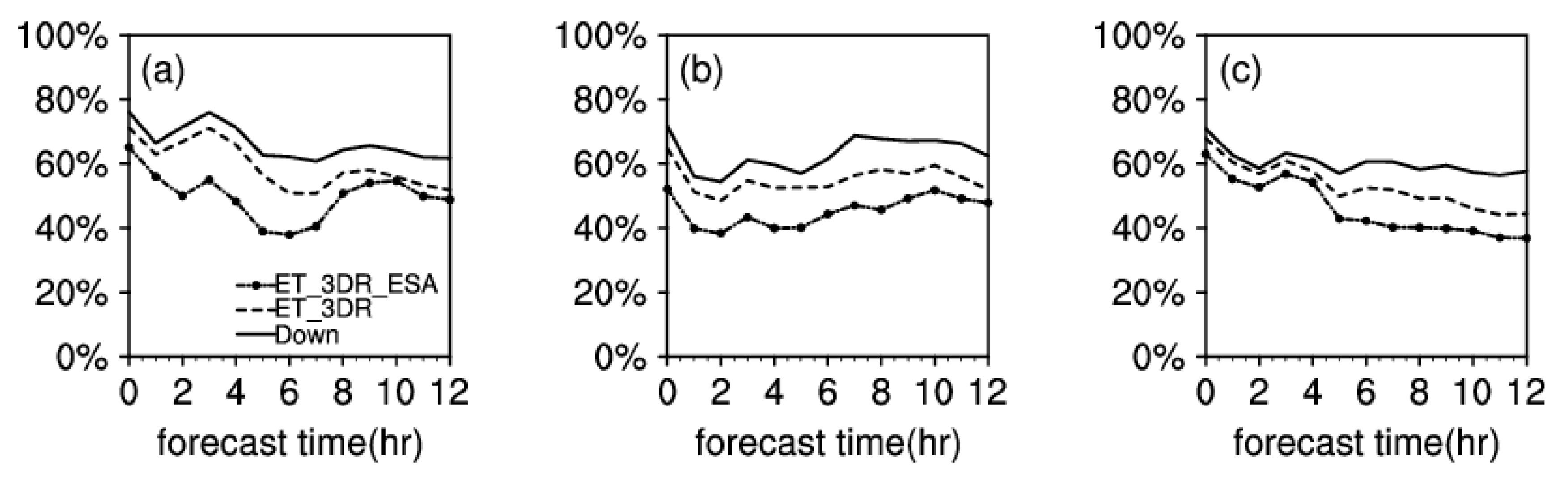
In order to further verify the reliability of the three ensemble forecast systems, the percentage of outliers was evaluated and compared; this is a statistic for the number of cases when the verifying analysis at any grid point lies outside the whole ensemble. The reliability of the ensemble forecast system increases as the percentage of outliers approaches , where n is the ensemble size [4].
Figure 6 shows the percentages of outliers for the values of T, U, and V for the three experiments under the 500-hPa condition. Before the occurrence of the squall line, the percentages of outliers for all three variables were within the range of 60–70%. However, as the squall line developed, the percentage exhibited a downward trend, decreasing by approximately 10% at the end of the forecast; these results indicate that all three of these ensemble forecast systems have a certain degree of reliability. Comparing the results of all three experiments revealed that the percentage of outliers for ET_3DR_ESA is lower than that of the other two experiments, thereby confirming that the ensemble members generated by ET_3DR_ESA can accurately represent the environmental conditions. In addition, the RMSE and percentage of outlier temperature results exhibited similar trends, suggesting that the temperature is particularly sensitive to squall line development.
A reasonable and effective ensemble forecast system is necessary to obtain comprehensive information on analysis uncertainties, i.e., both larger-scale and smaller-scale information [10]. Therefore, the two-dimensional discrete cosine transform (2D-DCT) [33] method was used to perform power spectrum analysis.
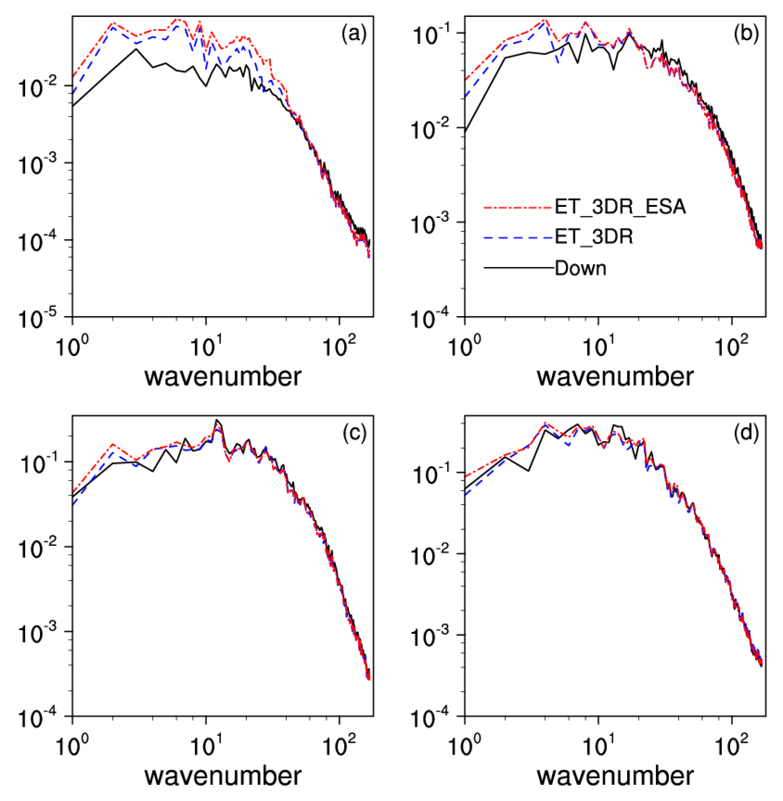
Figure 7 shows the 3-, 6-, 9-, and 12-h power spectrums for 850-hPa total energy as a function of the wavenumber for each of the three experiments. In the early forecast period, the power of Down is significantly less than that of the other two experiments. As the squall line developed, the scale-related features of all three experiments become more similar, and the large-scale power significantly increased. However, ET_3DR_ESA was found to have the highest power throughout the squall line development; this indicates that ET_3DR_ESA effectively reduces the dissipation of total energy on all scales. In addition, the small-scale power results for all experiments showed good stability at 6-h post-squall line occurrence, and the large-scale power results showed an increasing trend; these results suggests that, as a squall line develops, the total energy tends to propagate to the large scale.
3.3. Subjective Evaluation of the Precipitation Forecasts
Unlike temperature, which tends to mimic a Gaussian distribution, precipitation forecasts tend toward a positively skewed distribution [34]. Because a simple ensemble mean (EM) of precipitation may smooth out the peak values of precipitation, especially for extreme rainfall events [35], Ebert [36] proposed the probability matched (PM) method. The PM mean can yield the most accurate intensity, shape, and distribution forecasts for heavy rain. It is calculated as follows:
Here, n is the ensemble size and m is the total number of grid points. The variable x contains the precipitation amounts for all ensemble members at all grid points which have been sorted in descending order. and denote the simple ensemble mean and the PM mean, respectively. In order to obtain the PM mean, a new variable with the same size of is picked out of every n values from x. Then, the simple EM at each grid point is computed and then sorted at all grid points from largest to smallest into the variable . Finally, beginning from the grid point with the largest EM value in , the largest value of is taken as the PM mean value of this grid point and put it into . All grid points are then calculated to yield the PM mean field, . It should be noted that, when the EM value of a grid point is zero, the corresponding PM mean value must also be zero in order to maintain the same PM mean and EM field structure.
In recent years, the PM mean has been widely implemented in SSEF [35,37]; the corresponding reports show that the PM mean is capable of realizing forecasts that are more accurate than those resulting from use of the traditional ensemble mean.
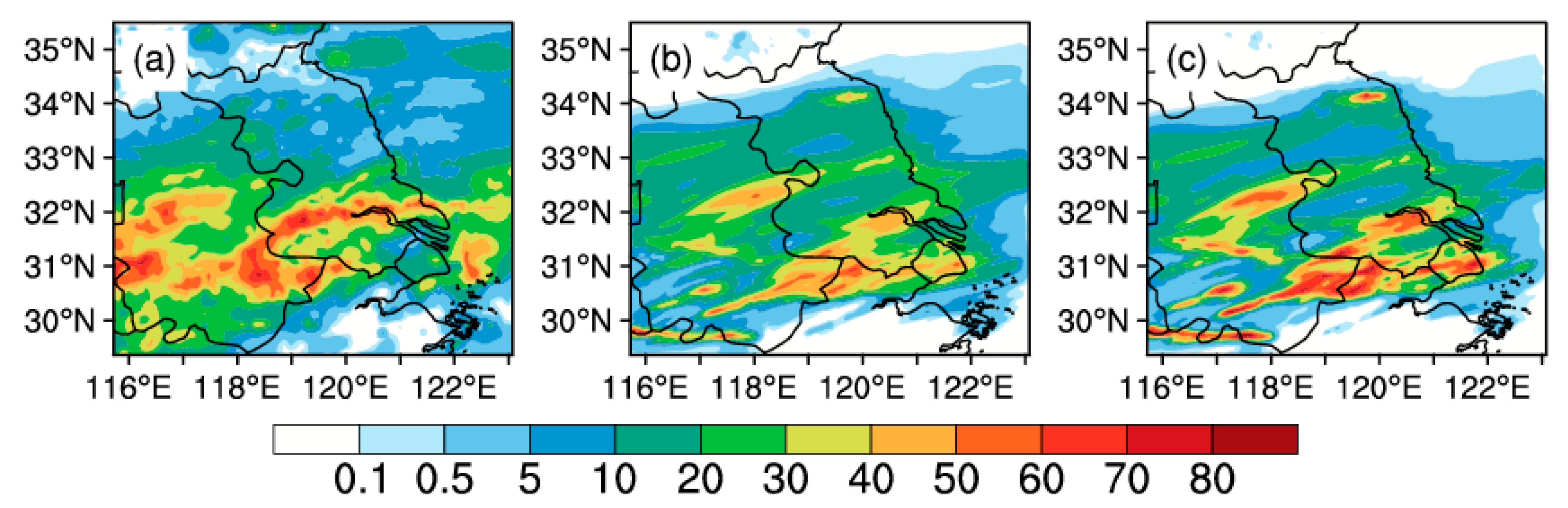
To verify that use of the PM mean improves forecasts related to regional precipitation and the intensity of squall line development, the EM and PM mean were used to forecast the 12-h accumulated precipitation that was observed from 0000 UTC to 1200 UTC on 12 July 2014; the results and their respective comparisons to the observed amount of precipitation are shown in Figure 8.
There are two large precipitation regions in the observation. One was located in western Anhui, and the other, shown as a circular precipitation region, was located in southeastern Anhui. Comparison of the EM and PM mean revealed the EM-based precipitation forecast to be significantly less than the observed amount; in general, this results in an underestimation of the amount of rainfall. Considering the diversified ability of ensemble members to forecast precipitation intensity and location, the PM mean can better capture the intensity and spatial distribution of precipitation; this is evidenced by the fact that the PM mean-based results match well with the observed result for the heavy precipitation that occurred in southeastern Anhui.
In general, the PM mean algorithm ensures that the maximum value of the PM mean at all grid points is near the maximum value of all ensemble members. Thus, the domain using the PM mean should only cover the related precipitation systems [35]. However, in this study, the PM mean achieved a satisfying level of performance under the conditions of a squall line with a relatively narrow and long precipitation band. Thus, if the PM mean is applied to forecast the amount of precipitation occurring in isolated convective systems, it will yield better performance.
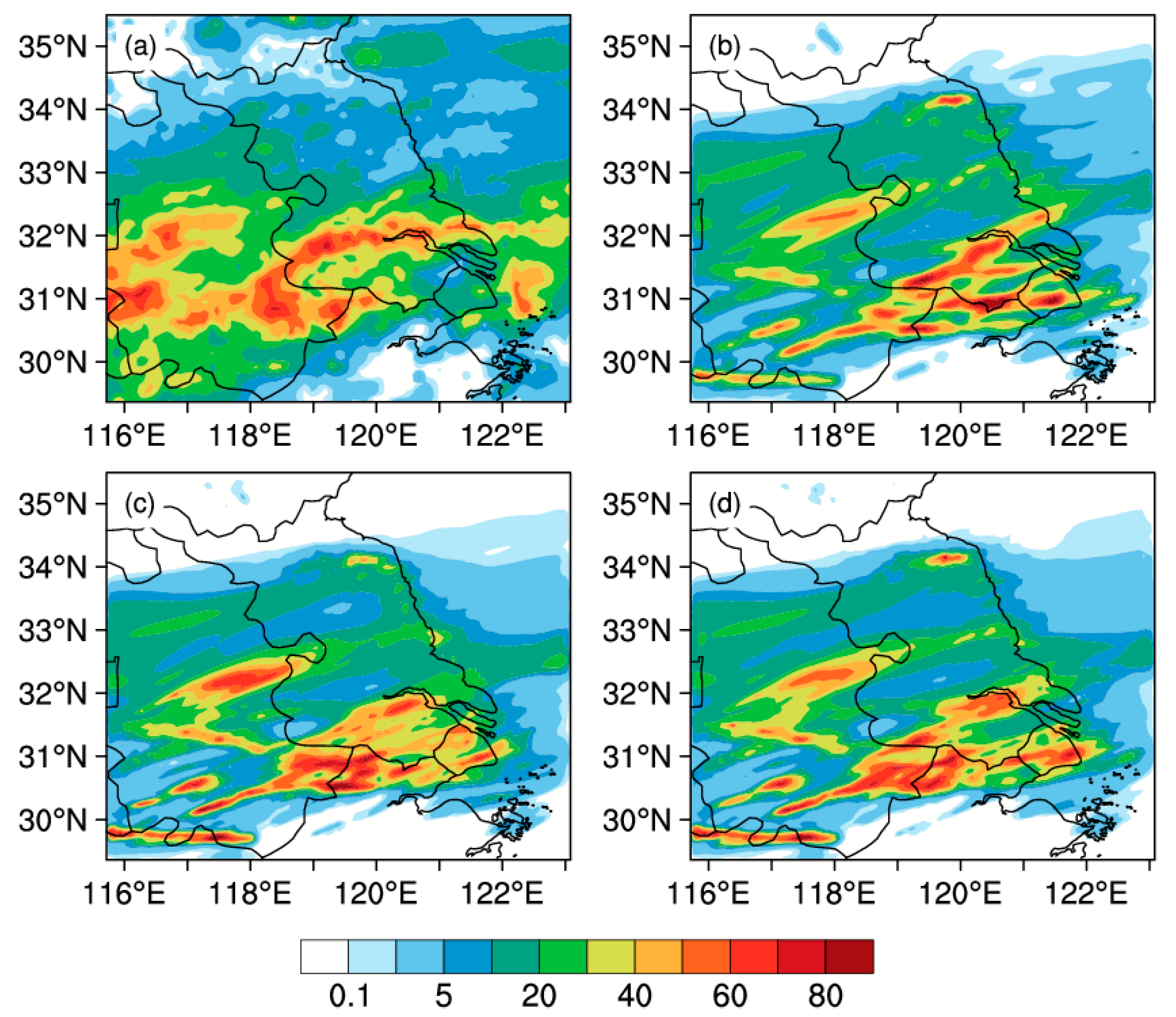
After evaluating the performance of the PM mean, the PM mean-based 12-h accumulated precipitation forecasts for the three representative experiments were compared to the observed precipitation amount (Figure 9). None of the three experiments were able to accurately forecast the large precipitation region in western Anhui. The reason for this is that the region is located near the boundary of the analysis domain; it should be noted that lateral boundary perturbations were not considered for qualitative analysis. Comparison of the three experiments revealed that Down was unable to accurately forecast the heavy precipitation that occurred in southeastern Anhui, and that it overestimated the amount of precipitation in southern Jiangsu.
Conversely, the precipitation distribution forecasts from ET_3DR and ET_3DR_ESA were similar, yielding sufficiently accurate forecasts for the circular precipitation region. However, the ET_3DR_ESA forecast better matched the observed precipitation results for southeastern Anhui and southern Jiangsu. To quantify the pattern-matching improvements, the spatial correlation relative to observation has been analyzed (not shown) and the ET_3DR_ESA obtains the highest value of 0.531, overtaking that of ET_3DR (0.494) and Down (0.476). Therefore, ET_3DR_ESA tended to yield forecasts that were more accurate than the other two experiments, and was thus able to moderately improve the performance of precipitation forecasts.
3.4. Quantitative Evaluation of the Precipitation Forecasts
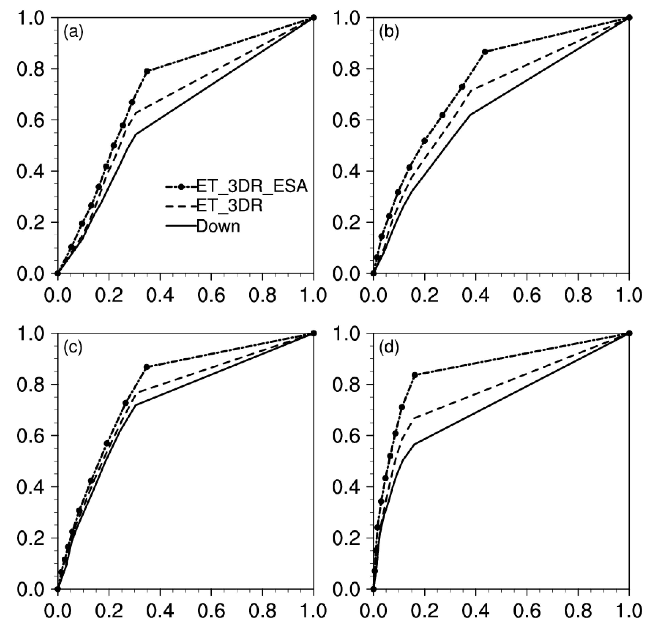
In this subsection, precipitation forecasts are evaluated by using several objective methods to verify the performances of the three representative ensemble forecast systems. The relative operating characteristic (ROC) test [38] is a commonly used method to measure the forecast performance for precipitation; when the ROC curve is closer to the Y axis, the precipitation forecast is more accurate.
Figure 10 shows the three ROC curves for 12-h accumulated precipitation and varying rain intensity. As can be seen, the ROC curves for the three experiments are consistently above the diagonal threshold line. This means that all three ensemble forecast systems are capable of forecasting with a certain degree of reliability. As compared to the other two experiments, the ROC curves for ET_3DR_ESA are consistently closer to the Y axis; this means that this method yields more accurate precipitation forecasts. However, all three experiments realized an acceptable forecast performance level under extreme rain conditions. Considering the conditions of the squall line utilized in this study, these results are relatively satisfying. It is worth noting that a similar trend in the ROC curves was observed for all rain intensities; this is possibly due to the squall line itself having high predictability, which minimized the differences related to the location of the precipitation forecast.
The Brier score (BS) [39] was used to measure the mean-square error between the probabilistic forecast and the actual observation, with a value of zero indicating a perfect system. It is calculated as follows:
Here, N is the ensemble size, and are forecast probability and observation probability for each gird point. For a specific threshold, if a grid point in the observation meet the threshold, then equals one. Otherwise, it is zero.
Unlike the BS, the equitable threat score (ETS) [40] is a deterministic score method. Its advantage lies in the punishment of misses and false alarms. Furthermore, in contrast to the BS, a perfect system has an ETS value of one. It is calculated as follows:
Here, total is the total number of grid points. , , and denote the number of grid points of hits, misses and false alarms, respectively. The BS and ETS were employed to further verify and evaluate the precipitation forecasts by obtaining a probabilistic and deterministic score.
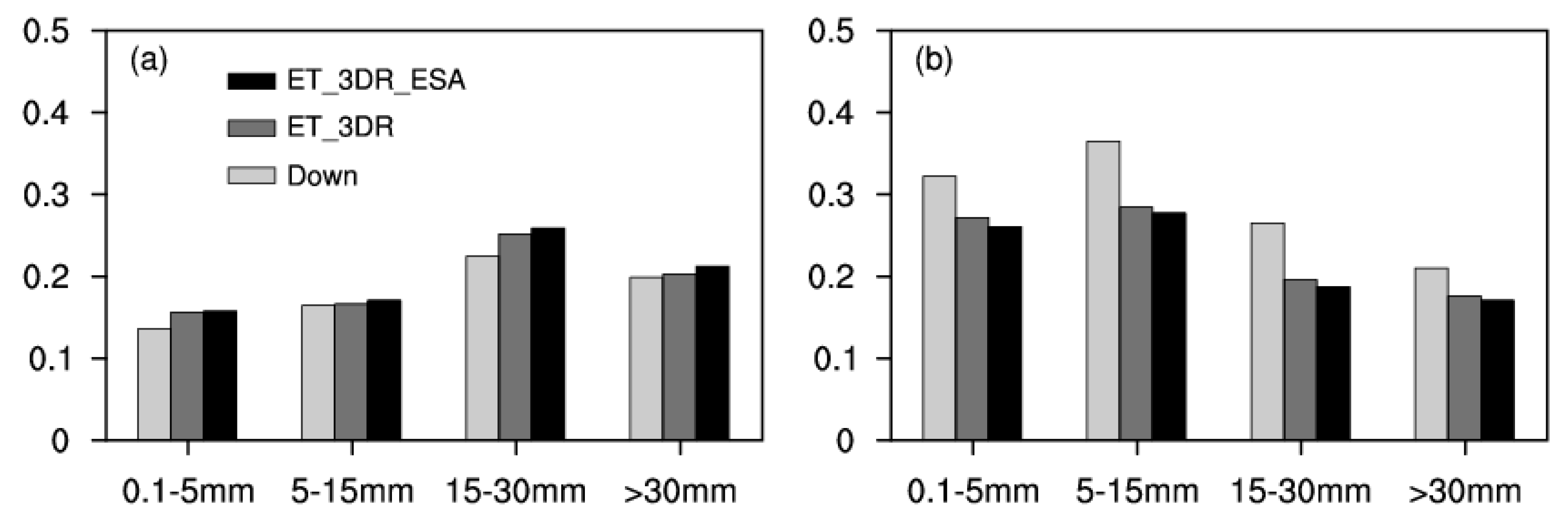
The ETS and BS for varying levels of 12-h accumulated precipitation are shown in Figure 11 for all three experiments. As was observed in the ROC curve results, the ETS and BS results corresponded to relatively accurate forecasts for all three experiments under the conditions of heavy and extreme rain. As can be seen in Figure 11, ET_3DR_ESA yielded the highest ETS and lowest BS for all four rain intensities; this means that the precipitation forecast produced by ET_3DR_ESA is more reliable. Additionally, neither the BS nor the ETS of ET_3DR_ESA was significantly improved compared to that of ET_3DR; this is due to the similar distribution of the precipitation forecasts that was mentioned in Section 3.2.
4. Conclusions
In order to develop ensemble generation methods for SSEF systems, three ensemble forecast experiments for a squall line that occurred in the Jianghuai region of China were carried out as based on the Down, ET_3DR, and ET_3DR_ESA methods. The features of ESA were investigated, and a quantitative evaluation of the ensemble forecasts, and subjective and quantitative evaluations of precipitation forecasts, were performed in order to evaluate the effectiveness of combining ET_3DR and ESA to produce initial perturbations in SSEF systems.
It was found that by analyzing the thermodynamic and moisture sensitivity, ESA was able to provide information about finer-scale features, while also being able to maintain a relationship with the synoptic-scale; furthermore, ESA can be used to generate initial perturbations that are in agreement with the synoptic conditions. In addition, measures such as ensemble spread, RMSE, the percentage of outliers, and the power spectrum were applied to evaluate three ensemble forecast systems. The results indicated that as the squall line developed, ET_3DR_ESA yielded the fastest spread growth, lowest RMSE, and lowest percentage of outliers, especially during the peak period of the squall line; these results suggest that, of the three ensemble forecast systems evaluated in this study, ET_3DR_ESA achieved the best performance. Moreover, the fact that ET_3DR_ESA achieved the highest power throughout the squall line process implies that ET_3DR_ESA effectively reduced the dissipation of total energy on all scales; additionally, the increasing trend of large-scale power indicates that the total energy tended to propagate to the large scale.
In addition, the PM mean method was estimated to achieve better precipitation forecast performance than the EM method. Comparing these two methods revealed that the PM mean yielded better forecasts for the precipitation intensity and distribution. Overall, comparing the three ensemble forecast systems revealed that ET_3DR_ESA was able to more accurately forecast the precipitation location and intensity of the circular precipitation region in southeastern Anhui. Additionally, to further improve the performance of precipitation forecasts, the ROC test, deterministic score ETS, and probabilistic BS were performed and used to respectively evaluate each of the three ensemble forecast systems. The results demonstrated that ET_3DR_ESA was best able to forecast the precipitation conditions for all precipitation intensities, and that all three experiments achieved relatively high forecast accuracy under the conditions of heavy and extreme rain, which is meaningful for storm-scale systems.
In this study, by using a squall line in the Jianghuai region as a reference, and by considering the features of storm-scale systems, a new ensemble generation method that combines ET_3DR and ESA was introduced for application to SSEF systems. The applicability of an ET_3DR_ESA-based storm-scale ensemble forecast was discussed in detail. The results showed that although ET_3DR is capable of achieving relatively good performance, perturbations controlled by ESA were able to improve the reliability of the ensemble forecast system.
Bednarczyk et al. [21] showed that ESA provided a measure of forecast sensitivity that intrinsically possessed error growth dynamics. Li et al. [41] focused on the short-range Numerical Weather Prediction of warm-season mesoscale systems over south-west China with the ESA method, and found that the ESA method helped to improve the movement and intensity forecast of Southwest Vortex. Therefore, ET_3DR_ESA may also be effective for another event. However, further work needs to concentrate on the relationship between the error growth features of ET_3DR_ESA and severe convective systems with varying predictability and features. In addition, because lateral boundary perturbations help improve ensemble spread [42], the introduction of lateral boundary perturbations, and how to improve their compatibility with initial perturbations, will also be further investigated.
Author Contributions
Y.F. conceived and designed the experiment. The paper was written by Y.F. with an important contribution by J.M. X.Z. and S.W. analyzed the data and presented the results.
Acknowledgments
This work was primarily supported by the National Key Research and Development Program of China (Grant Nos. 2017YFC1502103), the National Science Foundation of China (Grant No. 41430427), National Natural Science Foundation of China (G41805016, G41805070), Natural Science Foundation of Jiangsu Province (BK20170940, BK20160954), the Open Project of the Key Laboratory of Meteorological Disaster of Ministry of Education, Nanjing University of Information Science and Technology (KLME201807, KLME201808), Beijige Funding from Jiangsu Research Institute of Meteorological Science (BJG201604).
Conflicts of Interest
The authors declare no conflict of interest.
References
- Zhu, Y.; Ma, J. Predictability, Probabilistic Forecasting and Ensemble Prediction System; Lecture Notes on Numerical Weather Prediction; WMO Regional Training Center, NUIST: Nanjing, China, 2010; pp. 43–60. [Google Scholar]
- Toth, Z.; Kalnay, E. Ensemble Forecasting at NCEP and the Breeding Method. Mon. Weather Rev. 1997, 125, 3297–3319. [Google Scholar] [CrossRef] [Green Version]
- Wang, X.; Bishop, C.H. A Comparison of Breeding and Ensemble Transform Kalman Filter Ensemble Forecast Schemes. J. Atmos. Sci. 2003, 60, 1140–1158. [Google Scholar] [CrossRef]
- Wang, Y.; Bellus, M.; Geleyn, J.-F.; Ma, X.; Tian, W.; Weidle, F. A New Method for Generating Initial Condition Perturbations in a Regional Ensemble Prediction System: Blending. Mon. Weather Rev. 2014, 142, 2043–2059. [Google Scholar] [CrossRef]
- Ray, P.S.; Johnson, B.C.; Johnson, K.W.; Bradberry, J.S.; Stephens, J.J.; Wagner, K.; Wilhelmson, R.B.; Klemp, J.B. The Morphology of Several Tornadic Storms on 20 May 1977. J. Atmos. Sci. 1981, 38, 1643–1663. [Google Scholar] [CrossRef] [Green Version]
- Gebhardt, C.; Theis, S.E.; Paulat, M.; Ben Bouallègue, Z. Uncertainties in COSMO-DE precipitation forecasts introduced by model perturbations and variation of lateral boundaries. Atmos. Res. 2011, 100, 168–177. [Google Scholar] [CrossRef]
- Tennant, W. Improving initial condition perturbations for MOGREPS-UK: Improving Initial Condition Perturbations for MOGREPS-UK. Q. J. R. Meteorol. Soc. 2015, 141, 2324–2336. [Google Scholar] [CrossRef]
- Ma, J.; Zhu, Y.; Hou, D.; Zhou, X.; Peña, M. Ensemble Transform with 3D Rescaling Initialization Method. Mon. Weather Rev. 2014, 142, 4053–4073. [Google Scholar] [CrossRef]
- Szintai, B.; Ihász, I. The dynamical downscaling of ECMWF EPS products with the ALADIN mesoscale limited area model: Preliminary evaluation. Idojárás 2006, 110, 253–277. [Google Scholar]
- Craig, G.C.; Keil, C.; Leuenberger, D. Constraints on the impact of radar rainfall data assimilation on forecasts of cumulus convection. Q. J. R. Meteorol. Soc. 2012, 138, 340–352. [Google Scholar] [CrossRef]
- Wei, M.; Toth, Z.; Wobus, R.; Zhu, Y. Initial perturbations based on the ensemble transform (ET) technique in the NCEP global operational forecast system. Tellus A Dyn. Meteorol. Oceanogr. 2008, 60, 62–79. [Google Scholar] [CrossRef]
- Wang, X.; Parrish, D.; Kleist, D.; Whitaker, J. GSI 3DVar-Based Ensemble Variational Hybrid Data Assimilation for NCEP Global Forecast System: Single-Resolution Experiments. Mon. Weather Rev. 2013, 141, 4098–4117. [Google Scholar] [CrossRef]
- Hill, A.J.; Weiss, C.C.; Ancell, B.C. Ensemble Sensitivity Analysis for Mesoscale Forecasts of Dryline Convection Initiation. Mon. Weather Rev. 2016, 144, 4161–4182. [Google Scholar] [CrossRef]
- Torn, R.D.; Hakim, G.J. Ensemble-Based Sensitivity Analysis. Mon. Weather Rev. 2008, 136, 663–677. [Google Scholar] [CrossRef] [Green Version]
- Chang, E.K.M.; Zheng, M.; Raeder, K. Medium-Range Ensemble Sensitivity Analysis of Two Extreme Pacific Extratropical Cyclones. Mon. Weather Rev. 2013, 141, 211–231. [Google Scholar] [CrossRef]
- McMurdie, L.A.; Ancell, B. Predictability Characteristics of Landfalling Cyclones along the North American West Coast. Mon. Weather Rev. 2014, 142, 301–319. [Google Scholar] [CrossRef]
- Torn, R.D. Ensemble-Based Sensitivity Analysis Applied to African Easterly Waves. Weather Forecast. 2010, 25, 61–78. [Google Scholar] [CrossRef]
- Ito, K.; Wu, C.-C. Typhoon-Position-Oriented Sensitivity Analysis. Part I: Theory and Verification. J. Atmos. Sci. 2013, 70, 2525–2546. [Google Scholar] [CrossRef]
- Xie, B.; Zhang, F.; Zhang, Q.; Poterjoy, J.; Weng, Y. Observing Strategy and Observation Targeting for Tropical Cyclones Using Ensemble-Based Sensitivity Analysis and Data Assimilation. Mon. Weather Rev. 2013, 141, 1437–1453. [Google Scholar] [CrossRef]
- Torn, R.D. The Impact of Targeted Dropwindsonde Observations on Tropical Cyclone Intensity Forecasts of Four Weak Systems during PREDICT. Mon. Weather Rev. 2014, 142, 2860–2878. [Google Scholar] [CrossRef]
- Bednarczyk, C.N.; Ancell, B.C. Ensemble Sensitivity Analysis Applied to a Southern Plains Convective Event. Mon. Weather Rev. 2015, 143, 230–249. [Google Scholar] [CrossRef]
- Berman, J.D.; Torn, R.D.; Romine, G.S.; Weisman, M.L. Sensitivity of Northern Great Plains Convection Forecasts to Upstream and Downstream Forecast Errors. Mon. Weather Rev. 2017, 145, 2141–2163. [Google Scholar] [CrossRef]
- Torn, R.D.; Romine, G.S.; Galarneau, T.J. Sensitivity of Dryline Convection Forecasts to Upstream Forecast Errors for Two Weakly Forced MPEX Cases. Mon. Weather Rev. 2017, 145, 1831–1852. [Google Scholar] [CrossRef] [Green Version]
- Wile, S.M.; Hacker, J.P.; Chilcoat, K.H. The Potential Utility of High-Resolution Ensemble Sensitivity Analysis for Observation Placement during Weak Flow in Complex Terrain. Weather Forecast. 2015, 30, 1521–1536. [Google Scholar] [CrossRef]
- Hong, S.-Y.; Dudhia, J.; Chen, S.-H. A Revised Approach to Ice Microphysical Processes for the Bulk Parameterization of Clouds and Precipitation. Mon. Weather Rev. 2004, 132, 103–120. [Google Scholar] [CrossRef] [Green Version]
- Hong, S.-Y.; Noh, Y.; Dudhia, J. A New Vertical Diffusion Package with an Explicit Treatment of Entrainment Processes. Mon. Weather Rev. 2006, 134, 2318–2341. [Google Scholar] [CrossRef] [Green Version]
- Mlawer, E.J.; Taubman, S.J.; Brown, P.D.; Iacono, M.J.; Clough, S.A. Radiative transfer for inhomogeneous atmospheres: RRTM, a validated correlated-k model for the longwave. J. Geophys. Res. Atmos. 1997, 102, 16663–16682. [Google Scholar] [CrossRef] [Green Version]
- Dudhia, J. Numerical Study of Convection Observed during the Winter Monsoon Experiment Using a Mesoscale Two-Dimensional Model. J. Atmos. Sci. 1989, 46, 3077–3107. [Google Scholar] [CrossRef] [Green Version]
- Kain, J.S.; Fritsch, J.M. A One-Dimensional Entraining/Detraining Plume Model and Its Application in Convective Parameterization. J. Atmos. Sci. 1990, 47, 2784–2802. [Google Scholar] [CrossRef] [Green Version]
- Ancell, B.; Hakim, G.J. Comparing Adjoint- and Ensemble-Sensitivity Analysis with Applications to Observation Targeting. Mon. Weather Rev. 2007, 135, 4117–4134. [Google Scholar] [CrossRef] [Green Version]
- Dey, S.R.A.; Leoncini, G.; Roberts, N.M.; Plant, R.S.; Migliorini, S. A Spatial View of Ensemble Spread in Convection Permitting Ensembles. Mon. Weather Rev. 2014, 142, 4091–4107. [Google Scholar] [CrossRef]
- Fortin, V.; Abaza, M.; Anctil, F.; Turcotte, R. Why Should Ensemble Spread Match the RMSE of the Ensemble Mean? J. Hydrometeorol. 2014, 15, 1708–1713. [Google Scholar] [CrossRef]
- Denis, B.; Côté, J.; Laprise, R. Spectral Decomposition of Two-Dimensional Atmospheric Fields on Limited-Area Domains Using the Discrete Cosine Transform (DCT). Mon. Weather Rev. 2002, 130, 1812–1829. [Google Scholar] [CrossRef]
- Hamill, T.M.; Hagedorn, R.; Whitaker, J.S. Probabilistic Forecast Calibration Using ECMWF and GFS Ensemble Reforecasts. Part II: Precipitation. Mon. Weather Rev. 2008, 136, 2620–2632. [Google Scholar] [CrossRef]
- Zhu, K.; Xue, M. Evaluation of WRF-based convection-permitting multi-physics ensemble forecasts over China for an extreme rainfall event on 21 July 2012 in Beijing. Adv. Atmos. Sci. 2016, 33, 1240–1258. [Google Scholar] [CrossRef]
- Ebert, E.E. Ability of a Poor Man’s Ensemble to Predict the Probability and Distribution of Precipitation. Mon. Weather Rev. 2001, 129, 2461–2480. [Google Scholar] [CrossRef]
- Clark, A.J.; Gallus, W.A.; Xue, M.; Kong, F. A Comparison of Precipitation Forecast Skill between Small Convection-Allowing and Large Convection-Parameterizing Ensembles. Weather Forecast. 2009, 24, 1121–1140. [Google Scholar] [CrossRef] [Green Version]
- Kharin, V.V.; Zwiers, F.W. Improved Seasonal Probability Forecasts. J. Clim. 2003, 16, 1684–1701. [Google Scholar] [CrossRef]
- Candille, G.; Talagrand, O. Evaluation of probabilistic prediction systems for a scalar variable. Q. J. R. Meteorol. Soc. 2005, 131, 2131–2150. [Google Scholar] [CrossRef] [Green Version]
- Brill, K.F.; Mesinger, F. Applying a General Analytic Method for Assessing Bias Sensitivity to Bias-Adjusted Threat and Equitable Threat Scores. Weather Forecast. 2009, 24, 1748–1754. [Google Scholar] [CrossRef]
- Li, J.; Du, J.; Zhang, D.-L.; Cui, C.; Liao, Y. Ensemble-based analysis and sensitivity of mesoscale forecasts of a vortex over southwest China: Mesoscale Ensemble Forecast Sensitivity of Southwest Vortex in China. Q. J. R. Meteorol. Soc. 2014, 140, 766–782. [Google Scholar] [CrossRef]
- Saito, K.; Seko, H.; Kunii, M.; Miyoshi, T. Effect of lateral boundary perturbations on the breeding method and the local ensemble transform Kalman filter for mesoscale ensemble prediction. Tellus A Dyn. Meteorol. Oceanogr. 2012, 64, 11594. [Google Scholar] [CrossRef]
Figure 1.
Schematic diagram illustrating the ET_3DR_ESA ensemble forecast system.

Figure 2.
12 July 2014, 0000 UTC to 0300 UTC results. (a) Spread of 3-h accumulated precipitation (unit: mm) and (b) 3-h accumulated precipitation (unit: mm). The black box indicates the response region.
Figure 2.
12 July 2014, 0000 UTC to 0300 UTC results. (a) Spread of 3-h accumulated precipitation (unit: mm) and (b) 3-h accumulated precipitation (unit: mm). The black box indicates the response region.

Figure 3.
12 July 2014, 0000 UTC results. (a) 500-hPa geopotential height (shaded and contoured, unit: dagpm) and 200-hPa wind (vectors, unit: m/s), (b) 850-hPa geopotential height and wind, (c) sensitivity of forecast variable R with respect to the 500-hPa temperature (shaded, unit: °C; the dashed area indicates that the sensitivity passed a 0.05-level significance test) and 500-hPa temperature (contoured, unit: °C), and (d) sensitivity of forecast variable R with respect to the 850-hPa temperature and 850-hPa temperature. The black box indicates the response region.

Figure 4.
12 July 2014, 0000 UTC results. (a) 500-hPa water vapor flux (vectors and shaded, unit: g/(s·cm·hPa)), (b) 850-hPa water vapor flux, (c) sensitivity of forecast variable R with respect to a 500-hPa water-vapor mixing ratio (shaded, unit: kg/kg, the dashed area indicates that the sensitivity passed a 0.05-level significance test) and a 500-hPa water-vapor mixing ratio (contoured, unit: kg/kg), and (d) sensitivity of forecast variable R with respect to an 850-hPa water-vapor mixing ratio and 850-hPa water-vapor mixing ratio. The black box indicates the response region.

Figure 5.
(a–c) Ensemble spread and (d–f) RMSE for the three ensemble forecast systems under 850-hPa conditions; (a,d) temperature T (unit: K), (b,e) zonal wind U (unit: m/s), and (c,f) radial wind V (unit: m/s).
Figure 5.
(a–c) Ensemble spread and (d–f) RMSE for the three ensemble forecast systems under 850-hPa conditions; (a,d) temperature T (unit: K), (b,e) zonal wind U (unit: m/s), and (c,f) radial wind V (unit: m/s).

Figure 6.
Percentage of outliers for the three ensemble forecast systems under 500-hPa conditions; (a) temperature T (unit: K), (b) zonal wind U (unit: m/s), and (c) radial wind V (unit: m/s).
Figure 6.
Percentage of outliers for the three ensemble forecast systems under 500-hPa conditions; (a) temperature T (unit: K), (b) zonal wind U (unit: m/s), and (c) radial wind V (unit: m/s).

Figure 7.
Power spectrum for 850-hPa total energy as a function of the wavenumber for the three ensemble forecast systems; (a) 3 h, (b) 6 h, (c) 9 h, and (d) 12 h.
Figure 7.
Power spectrum for 850-hPa total energy as a function of the wavenumber for the three ensemble forecast systems; (a) 3 h, (b) 6 h, (c) 9 h, and (d) 12 h.

Figure 8.
2-h accumulated precipitation distribution for 0000 UTC to 1200 UTC on 12 July 2014 (unit: mm); (a) observation, (b) EM, and (c) PM mean.
Figure 8.
2-h accumulated precipitation distribution for 0000 UTC to 1200 UTC on 12 July 2014 (unit: mm); (a) observation, (b) EM, and (c) PM mean.

Figure 9.
12-h accumulated precipitation distribution for 0000 UTC to 1200 UTC on 12 July 2014 (unit: mm); (a) observation, (b) Down, (c) ET_3DR, and (d) ET_3DR_ESA.
Figure 9.
12-h accumulated precipitation distribution for 0000 UTC to 1200 UTC on 12 July 2014 (unit: mm); (a) observation, (b) Down, (c) ET_3DR, and (d) ET_3DR_ESA.

Figure 10.
12-h accumulated precipitation relative operating characteristic (ROC) curves for the three ensemble forecast systems. (a) light rain (0.1–5 mm), (b) moderate rain (5–15 mm), (c) heavy rain (15–30 mm), and (d) extreme rain (>30 mm).
Figure 10.
12-h accumulated precipitation relative operating characteristic (ROC) curves for the three ensemble forecast systems. (a) light rain (0.1–5 mm), (b) moderate rain (5–15 mm), (c) heavy rain (15–30 mm), and (d) extreme rain (>30 mm).

Figure 11.
12-h accumulated precipitation (a) equitable threat score (ETS) and (b) Brier score (BS) for the three ensemble forecast systems.
Figure 11.
12-h accumulated precipitation (a) equitable threat score (ETS) and (b) Brier score (BS) for the three ensemble forecast systems.


Table 1.
Schemes for different ensemble forecast experiments.
| Experiment | Ensemble Generation Method | Members |
|---|---|---|
| Down | Dynamical downscaling method | 20 |
| ET_3DR | ET_3DR method | 20 |
| ET_3DR_ESA | Blending ET_3DR and ESA method | 20 |
© 2019 by the authors. Licensee MDPI, Basel, Switzerland. This article is an open access article distributed under the terms and conditions of the Creative Commons Attribution (CC BY) license (http://creativecommons.org/licenses/by/4.0/).
Share and Cite
MDPI and ACS Style
Feng, Y.; Min, J.; Zhuang, X.; Wang, S. Ensemble Sensitivity Analysis-Based Ensemble Transform with 3D Rescaling Initialization Method for Storm-Scale Ensemble Forecast. Atmosphere 2019, 10, 24. https://doi.org/10.3390/atmos10010024
AMA Style
Feng Y, Min J, Zhuang X, Wang S. Ensemble Sensitivity Analysis-Based Ensemble Transform with 3D Rescaling Initialization Method for Storm-Scale Ensemble Forecast. Atmosphere. 2019; 10(1):24. https://doi.org/10.3390/atmos10010024
Chicago/Turabian StyleFeng, Yuxuan, Jinzhong Min, Xiaoran Zhuang, and Shiqi Wang. 2019. "Ensemble Sensitivity Analysis-Based Ensemble Transform with 3D Rescaling Initialization Method for Storm-Scale Ensemble Forecast" Atmosphere 10, no. 1: 24. https://doi.org/10.3390/atmos10010024
Note that from the first issue of 2016, this journal uses article numbers instead of page numbers. See further details here.