A Review on a Deep Learning Perspective in Brain Cancer Classification

 ,
,
Abstract
:1. Introduction
2. Pathophysiology of Brain Cancer
2.1. Cellular Level Architecture
- (i)
- The first category is known as tumor suppressors that controls the cell death cycle (apoptosis) [14]. This process has two signaling pathways. In the first pathway, the signal is generated by a cell to kill itself while in the second, the cell receives the death signal from nearby cells. This process of cell death is slowed down by a mutation in one of the pathways. It stops completely if this mutation happens in both pathways, leading to unstoppable cell growth [14,15]. Some examples of cell suppressor genes are RB1, PTEN, which are responsible for cell death [16].
- (ii)
- The second category of genes is responsible for the repair of the DNA. Example of DNA repair genes are MGMT and p53 protein. Any malfunctioning in them may trigger cancer.
- (iii)
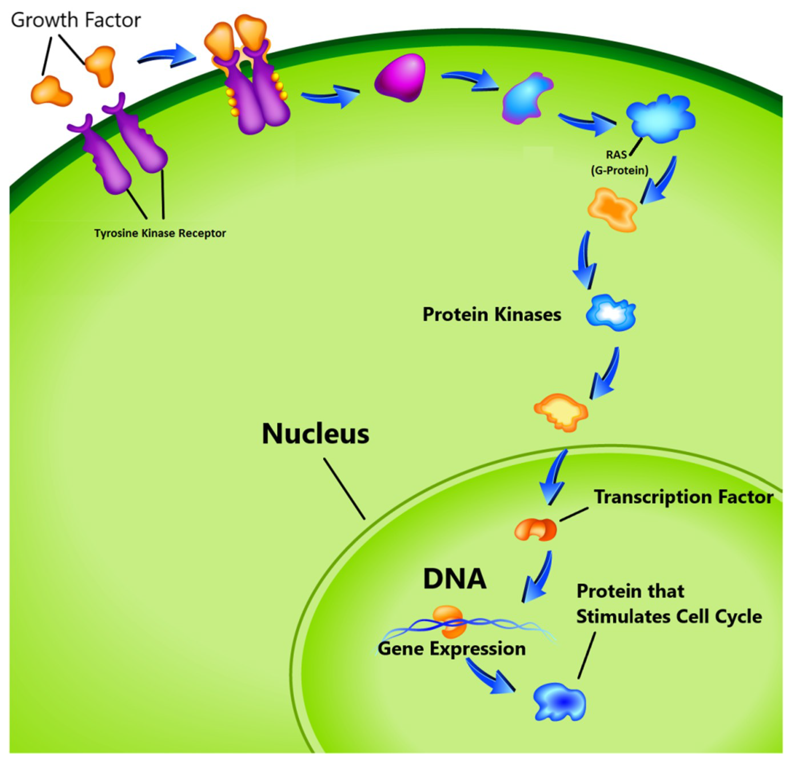
- The third group known as proto-oncogenes, are in opposition to the function of the tumor suppressor genes and are responsible for the production of the protein fostering the division process and inhibiting the normal cell death [17,18]. In healthy cells, the cell division cycle is controlled by proto-oncogenes via protein signals which are generated by the cell itself or the connected cells. Once the signal is generated, it goes through a series of different steps, which is called signal transduction cascade or pathway as shown in Figure 1. This signal may be generated by the cell itself or from the nearby cells that are directly connected to it. In this pathway, many proteins are involved to carry the signal from the cell membrane to nucleus through the cytoplasm. In this process the cell membrane receptor accepts the signal and carries the message to nucleolus through various intermediate factors. Once, the signal reaches to the nucleus, the responsible genes for transcription is activated and performs the cell division task. One of the known proto-oncogenes responsible for the transcription is RAS which acts as a switch to turn ‘on’ or ‘off’ the cell division process [19]. Mutation alters its functionality which leads to transform this gene into an oncogene. In this situation the gene is unable to switch off the cell division signal and unstoppable growth of the cells may begin.
2.2. Relevancy between Brain Tumor and Genes
3. Imaging Modality
3.1. Computed Tomography Imaging
3.2. Magnetic Resonance Imaging
3.3. Biopsy
3.4. Hyperstereoscopy Imaging
3.5. MR Spectroscopy
4. World Health Organization Guidelines for Tumor Grading
5. Brain Tumor Tests
5.1. Biomarker Test
5.2. Biopsy
5.3. Imaging Test
6. Classification Methods
6.1. Machine Learning
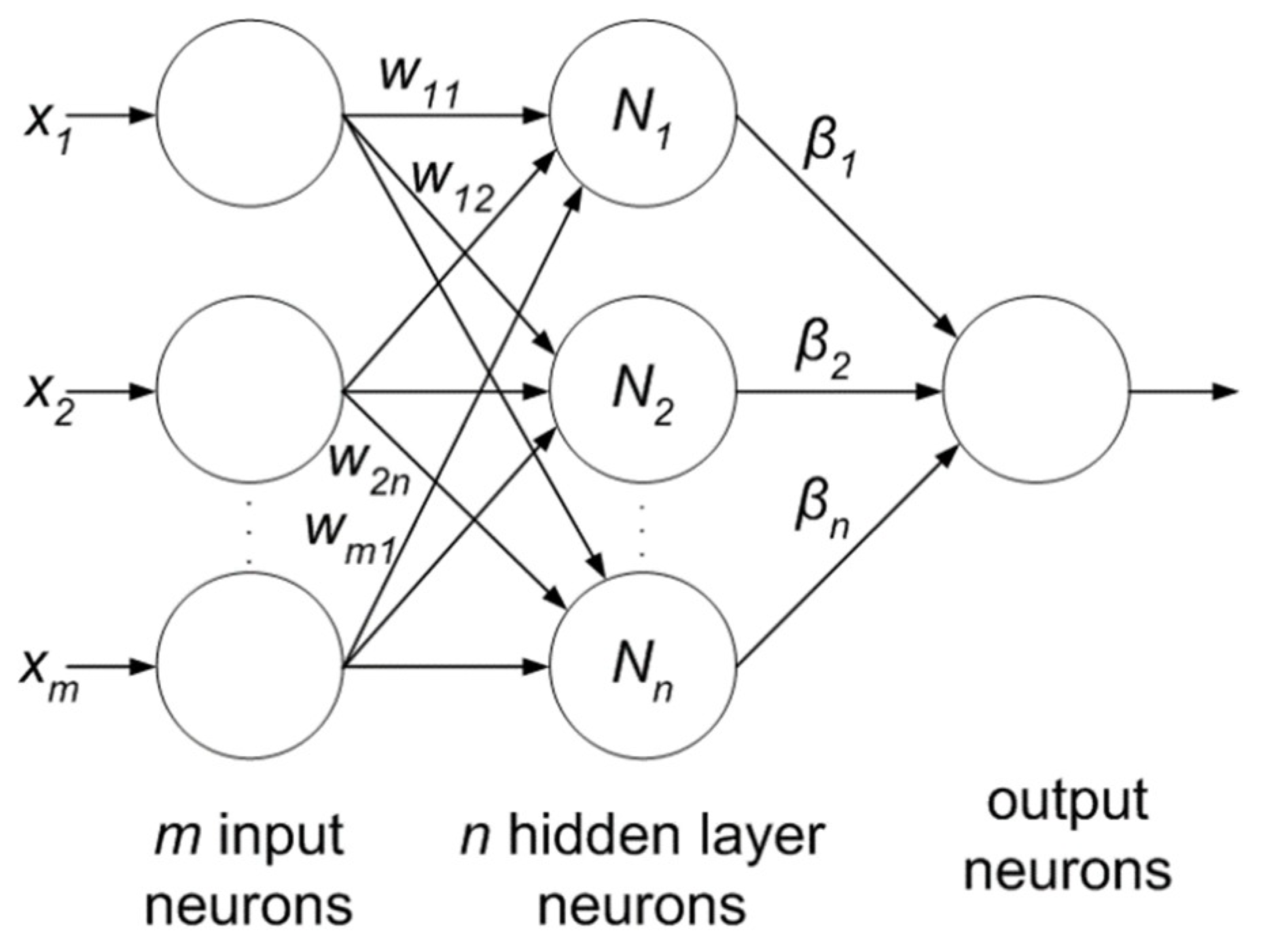
6.1.1. ANN-Based MRI Brain Tumor Classification Using Genetic Features
6.1.2. A Hybrid Characterization System for Brain Cancer Tumors
6.1.3. A Characterization System for Grading Brain Cancer Tumors
6.1.4. A Multi-Parametric Tissue Characterization System for Brain Neoplasm
6.1.5. Extreme Learning Machine
6.2. Deep Learning
6.2.1. Input Image Format
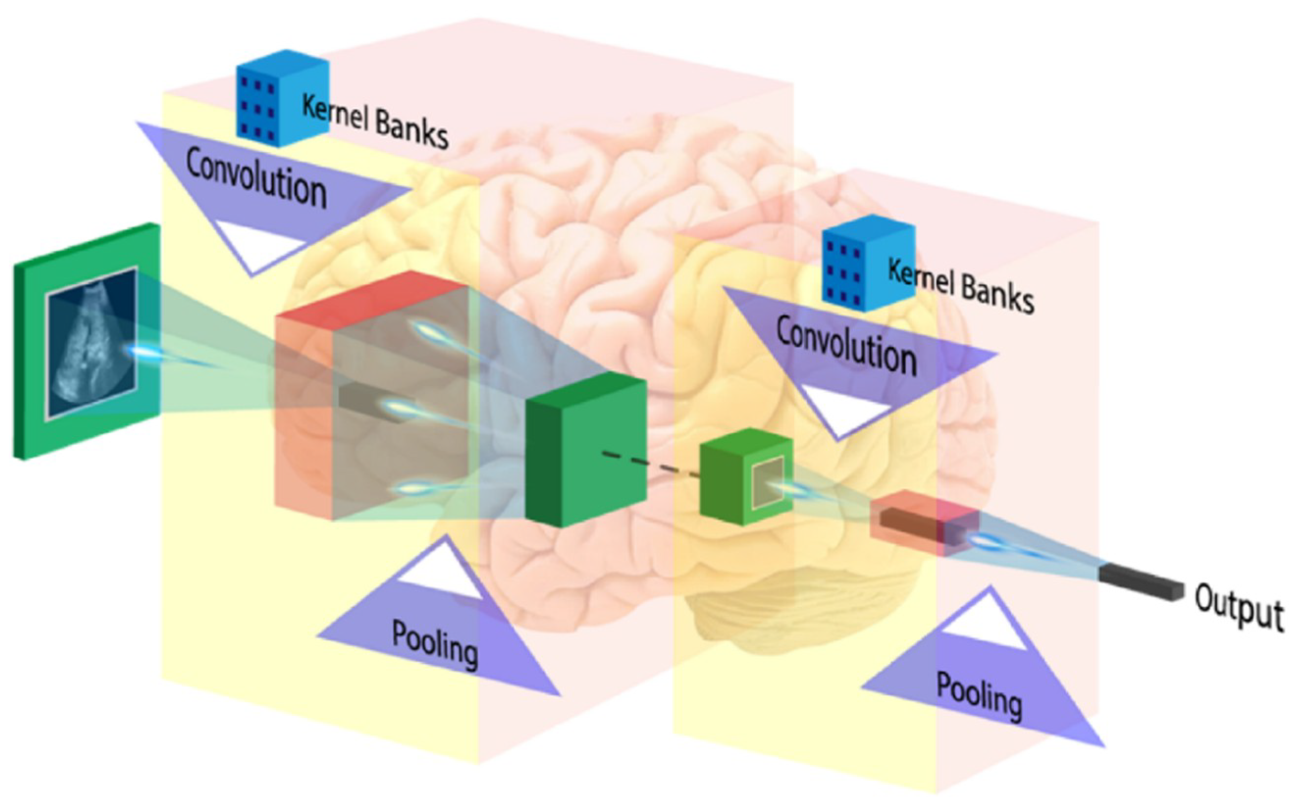
6.2.2. Convolution Layer
6.2.3. Activation Function
6.2.4. Pooling Layer
6.2.5. Fully Connected Layer
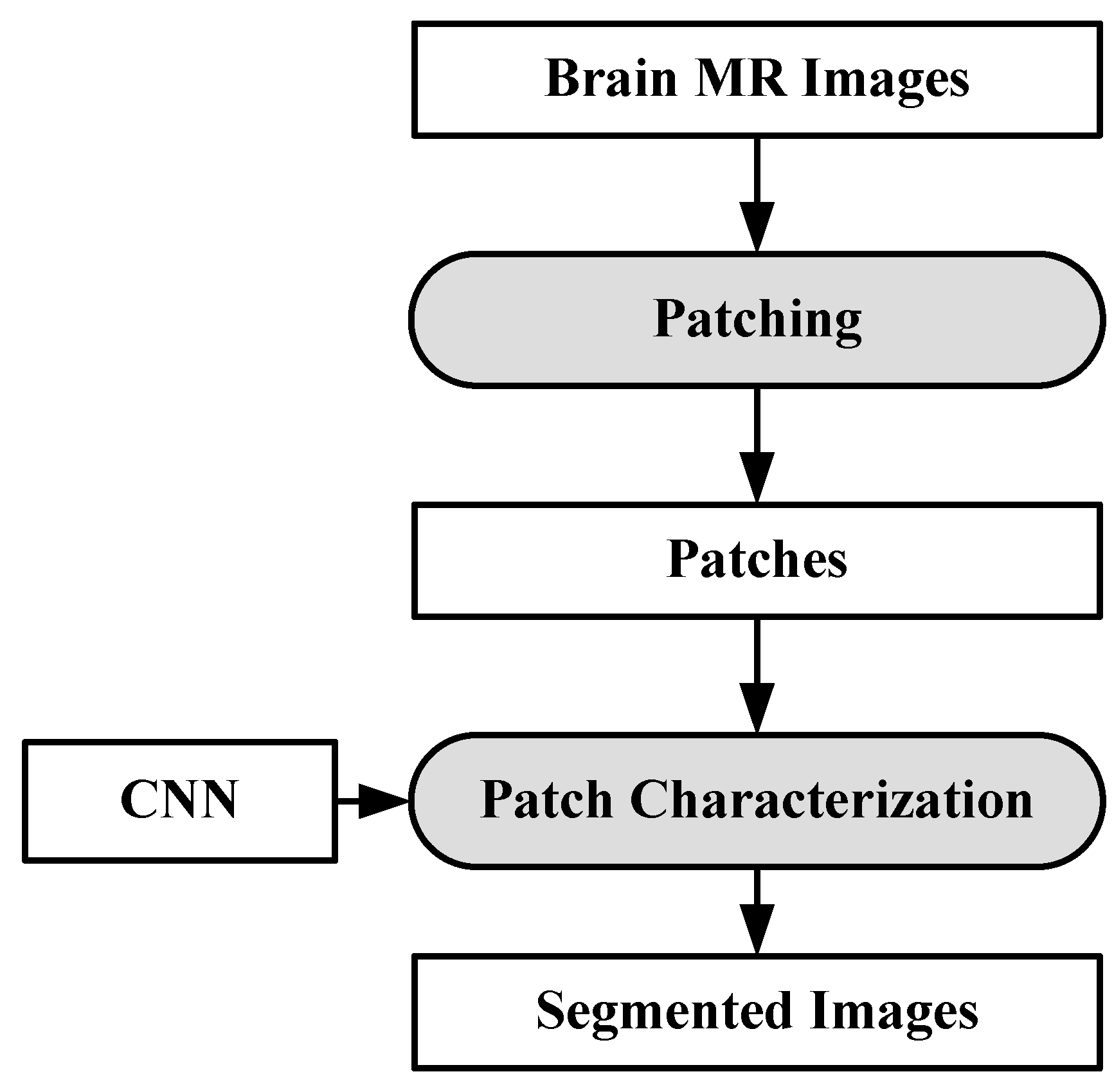
6.3. Brain Image Analysis Using Deep Learning
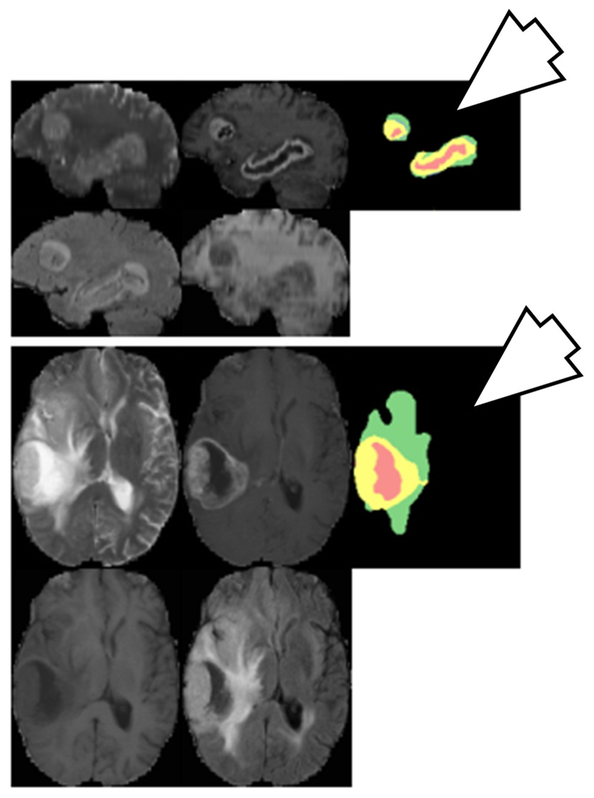
6.3.1. DL-Based Inter-Institutional Brain Tumor Segmentation
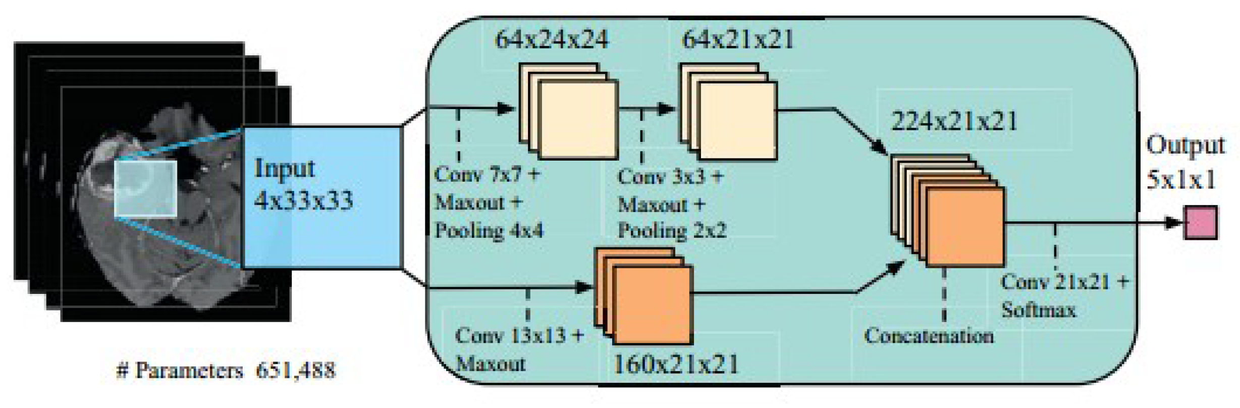
6.3.2. Brain Tumor Segmentation Using Two-Pathway CNN
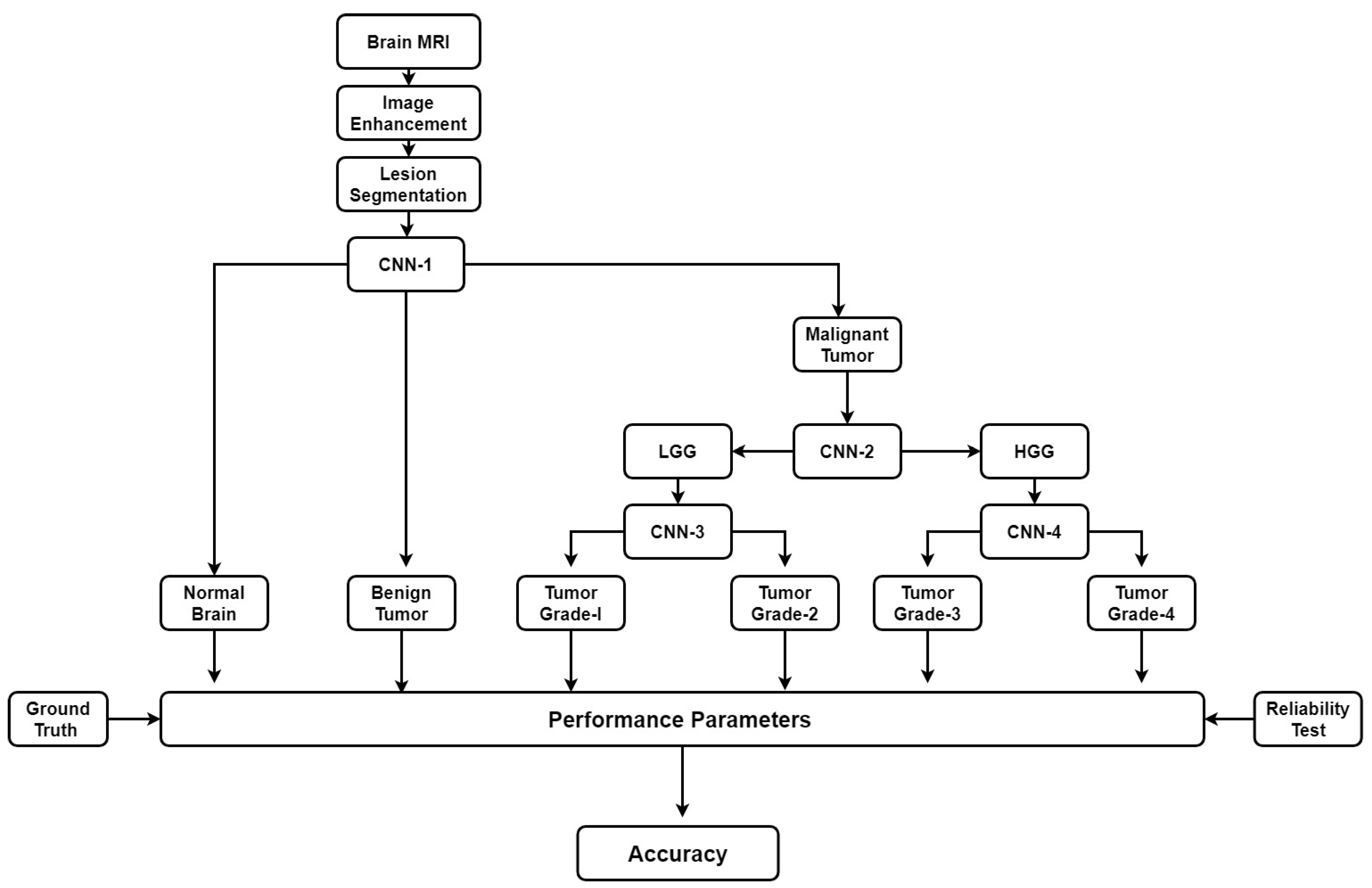
6.4. Plausible Solution for Brain Cancer Classification
7. Brain Cancer and Other Brain Disorders
7.1. Stroke
7.2. Alzheimer’s Disease
7.3. Parkinson’s Disease
7.4. Leukoaraiosis
7.5. Multiple Sclerosis
7.6. Wilson’s Disease
8. Discussion
8.1. A Note on Biomarkers for Cancer Detection
8.2. Benchmarking
9. Conclusions
Funding
Conflicts of Interest
References
- International Agency for Research on Cancer. Available online: https://gco.iarc.fr/ (accessed on 1 November 2018).
- Brain Tumor Basics. Available online: https://www.thebraintumourcharity.org/ (accessed on 1 November 2018).
- American Cancer Society website. Available online: www.cancer.org/cancer.html (accessed on 1 November 2018).
- Brain Tumor Diagnosis. Available online: https://www.cancer.net/cancer-types/brain-tumor/diagnosis (accessed on 1 November 2018).
- WHO Statistics on Brain Cancer. Available online: http://www.who.int/cancer/en/ (accessed on 1 November 2018).
- Shah, V.; Kochar, P. Brain Cancer: Implication to Disease, Therapeutic Strategies and Tumor Targeted Drug Delivery Approaches. Recent Pat. Anti-Cancer Drug Discov. 2018, 13, 70–85. [Google Scholar] [CrossRef] [PubMed]
- Ahmed, S.; Iftekharuddin, K.M.; ArastooVossoug. Efficacy of texture, shape, and intensity feature fusion for posterior-fossa tumor segmentation in MRI. IEEE Trans. Inf. Technol. Biomed. 2011, 15, 206–213. [Google Scholar] [CrossRef] [PubMed]
- Behin, A.; Hoang-Xuan, K.; Carpentier, A.F.; Delattre, J. Primary brain tumoursinadults. Lancet 2003, 361, 323–331. [Google Scholar] [CrossRef]
- Deorah, S.; Lynch, C.F.; Sibenaller, Z.A.; Ryken, T.C. Trends in brain cancer incidence and survival in the United States: Surveillance, Epidemiology, and End Results Program, 1973 to 2001. Neurosurg. Focus 2006, 20, E1. [Google Scholar] [CrossRef] [PubMed]
- Mahaley, M.S., Jr.; Mettlin, C.; Natarajan, N.; Laws, E.R., Jr.; Peace, B.B. National survey of patterns of care for brain-tumor patients. J. Neurosurg. 1989, 71, 826–836. [Google Scholar] [CrossRef]
- Hayward, R.M.; Patronas, N.; Baker, E.H.; Vézina, G.; Albert, P.S.; Warren, K.E. Inter-observer variability in the measurement of diffuse intrinsic pontine gliomas. J. Neuro-Oncol. 2008, 90, 57–61. [Google Scholar] [CrossRef] [Green Version]
- Griffiths, A.J.F.; Wessler, S.R.; Lewontin, R.C.; Gelbart, W.M.; Suzuki, D.T.; Miller, J.H. An Introduction to Genetic Analysis; Macmillan: New York, NY, USA, 2005. [Google Scholar]
- Shinoura, N.; Chen, L.; Wani, M.A.; Kim, Y.G.; Larson, J.J.; Warnick, R.E.; Simon, M.; Menon, A.G.; Bi, W.L.; Stambrook, P.J. Protein and messenger RNA expression of connexin43 in astrocytomas: Implications in brain tumor gene therapy. J. Neurosurg. 1996, 84, 839–845. [Google Scholar] [CrossRef] [PubMed]
- Evan, G.I.; Vousden, K.H. Proliferation, cell cycle and apoptosis in cancer. Nature 2001, 411, 342. [Google Scholar] [CrossRef]
- Burch, P.R. The Biology of Cancer: A New Approach; Springer Science & Business Media: New York, NY, USA, 2012. [Google Scholar]
- Song, M.S.; Salmena, L.; Pandolfi, P.P. The functions and regulation of the PTEN tumoursuppressor. Nat. Rev. Mol. CellBiol. 2012, 13, 283. [Google Scholar] [CrossRef]
- Rak, J.; Filmus, J.; Finkenzeller, G.; Grugel, S.; Marme, D.; Kerbel, R.S. Oncogenes as inducers of tumor angiogenesis. Cancer Metastasis Rev. 1995, 14, 263–277. [Google Scholar] [CrossRef]
- Yarden, Y.; Kuang, W.-J.; Yang-Feng, T.; Coussens, L.; Munemitsu, S.; Dull, T.J.; Chen, E.; Schlessinger, J.; Francke, U.; Ullrich, A. Human proto-oncogene c-kit: A new cell surface receptor tyrosine kinase for an unidentified ligand. EMBO J. 1987, 6, 3341–3351. [Google Scholar] [CrossRef]
- Greenberg, M.E.; Greene, L.A.; Ziff, E.B. Nerve growth factor and epidermal growth factor induce rapid transient changes in proto-oncogene transcription in PC12 cells. J. Biol. Chem. 1985, 260, 14101–14110. [Google Scholar] [PubMed]
- Sneed, P.K.; Suh, J.H.; Goetsch, S.J.; Sanghavi, S.N.; Chappell, R.; Buatti, J.M.; Regine, W.F.; Weltman, E.; King, V.J.; Breneman, J.C.; et al. A multi-institutional review of radiosurgery alone vs. radiosurgery with whole brain radiotherapy as the initial management of brain metastases. Int. J. Radiat. Oncol. Biol. Phys. 2002, 53, 519–526. [Google Scholar] [CrossRef]
- Bertram, J.S. The molecular biology of cancer. Mol. Asp. Med. 2000, 21, 167–223. [Google Scholar] [CrossRef]
- Liao, J.B. Cancer issue: Viruses and human cancer. Yale J. Biol. Med. 2006, 79, 115–122. [Google Scholar]
- Golemis, E.A.; Scheet, P.; Beck, T.N.; Scolnick, E.M.; Hunter, D.J.; Hawk, E.; Hopkins, N. Molecular mechanisms of the preventable causes of cancer in the United States. Genes Dev. 2018, 32, 868–902. [Google Scholar] [CrossRef] [PubMed]
- Swartling, F.J.; Čančer, M.; Frantz, A.; Weishaupt, H.; Persson, A.I. Deregulated proliferation and differentiation in brain tumors. Cell Tissue Res. 2015, 359, 225–254. [Google Scholar] [CrossRef]
- Montes-Mojarro, I.; Steinhilber, J.; Bonzheim, I.; Quintanilla-Martinez, L.; Fend, F. The Pathological Spectrum of Systemic Anaplastic Large Cell Lymphoma (ALCL). Cancers 2018, 10, 107. [Google Scholar] [CrossRef]
- Mabray, M.C.; Barajas, R.F.; Cha, S. Modern brain tumor imaging. Brain tumor research and treatment 2015, 3, 8–23. [Google Scholar] [CrossRef]
- Hegi, M.E.; Murat, A.; Lambiv, W.L.; Stupp, R. Brain tumors: Molecular biology and targeted therapies. Ann. Oncol. 2006, 17, x191–x197. [Google Scholar] [CrossRef]
- Yan, H.; Parsons, D.W.; Jin, G.; McLendon, R.; Rasheed, B.A.; Yuan, W.; Kos, I.; Batinic-Haberle, I.; Jones, S.; Riggins, G.J.; et al. IDH1 and IDH2 mutations in gliomas. N. Engl. J. Med. 2009, 360, 765–773. [Google Scholar] [CrossRef] [PubMed]
- Hu, N.; Richards, R.; Jensen, R. Role of chromosomal 1p/19q co-deletion on the prognosis of oligodendrogliomas: A systematic review and meta-analysis. Interdiscip. Neurosurg. 2016, 5, 58–63. [Google Scholar] [CrossRef] [Green Version]
- Lee, E.; Yong, R.L.; Paddison, P.; Zhu, J. Comparison of glioblastoma (GBM) molecular classification methods. In Seminars in Cancer Biology; Academic Press: New York, NY, USA, 2018. [Google Scholar] [CrossRef]
- Amyot, F.; Arciniegas, D.B.; Brazaitis, M.P.; Curley, K.C.; Diaz-Arrastia, R.; Gandjbakhche, A.; Herscovitch, P.; Hindsll, S.R.; Manley, G.T.; Pacifico, A.; et al. A review of the effectiveness of neuroimaging modalities for the detection of traumatic brain injury. J. Neurotrauma 2015, 32, 1693–1721. [Google Scholar] [CrossRef] [PubMed]
- Pope, W.B. Brain metastases: Neuroimaging. Handb. Clin. Neurol. 2018, 149, 89–112. [Google Scholar] [CrossRef] [PubMed]
- Morris, Z.; Whiteley, W.N.; Longstreth, W.T.; Weber, F.; Lee, Y.; Tsushima, Y.; Alphs, H.; Ladd, S.C.; Warlow, C.; Wardlaw, J.M.; et al. Incidental findings on brain magnetic resonance imaging: Systematic review and meta-analysis. BMJ 2009, 339, b3016. [Google Scholar] [CrossRef] [PubMed]
- Lagerwaard, F.; Levendag, P.C.; Nowak, P.J.C.M.; Eijkenboom, W.M.H.; Hanssens, P.E.J.; Schmitz, P.M. Identification of prognostic factors in patients with brain metastases: A review of 1292 patients. Int. J. Radiat. Oncol. Biol. Phys. 1999, 43, 795–803. [Google Scholar] [CrossRef]
- Smith-Bindman, R.; Lipson, J.; Marcus, R.; Kim, K.P.; Mahesh, M.; Gould, R.; de González, A.B.; Miglioretti, D.L. Radiation dose associated with common computed tomography examinations and the associated lifetime attributable risk of cancer. Arch. Intern. Med. 2009, 169, 2078–2086. [Google Scholar] [CrossRef] [PubMed]
- Dong, Q.; Welsh, R.C.; Chenevert, T.L.; Carlos, R.C.; Maly-Sundgren, P.; Gomez-Hassan, D.M.; Mukherji, S.K. Clinical applications of diffusion tensor imaging. J. Magn. Reson. Imaging 2004, 19, 6–18. [Google Scholar] [CrossRef]
- Khoo, M.M.Y.; Tyler, P.A.; Saifuddin, A.; Padhani, A.R. Diffusion-weighted imaging (DWI) in musculoskeletal MRI: A critical review. Skelet. Radiol. 2011, 40, 665–681. [Google Scholar] [CrossRef]
- Savoy, R.L. Functional magnetic resonance imaging (fMRI). In Encyclopedia of Neuroscience; Elsevier: Charlestown, MA, USA, 1999. [Google Scholar]
- Gurcan, M.N.; Boucheron, L.; Can, A.; Madabhushi, A.; Rajpoot, N.; Yener, B. Histopathological image analysis: A review. IEEE Rev. Biomed. Eng. 2009, 2, 147. [Google Scholar] [CrossRef]
- Fabelo, H.; Ortega, S.; Lazcano, R.; Madroñal, D.; M Callicó, G.; Juárez, E.; Salvador, R.; Bulters, D.; Bulstrode, H.; Szolna, A.; et al. An intraoperative visualization system using hyperspectral imaging to aid in brain tumor delineation. Sensors 2018, 18, 430. [Google Scholar] [CrossRef] [PubMed]
- Petersson, H.; Gustafsson, D.; Bergstrom, D. Hyperspectral image analysis using deep learning—A review. In Proceedings of the IEEE 2016 6th International Conference on Image Processing Theory Tools and Applications (IPTA), Oulu, Finland, 12–15 December 2016; pp. 1–6. [Google Scholar] [CrossRef]
- Lu, G.; Fei, B. Medical hyperspectral imaging: A review. J. Biomed. Opt. 2014, 19, 010901. [Google Scholar] [CrossRef] [PubMed]
- Halicek, M.; Lu, G.; Little, J.V.; Wang, X.; Patel, M.; Griffith, C.C.; El-Deiry, M.W.; Chen, A.Y.; Fei, B. Deep convolutional neural networks for classifying head and neck cancer using hyperspectral imaging. J. Biomed. Opt. 2017, 22, 060503. [Google Scholar] [CrossRef] [PubMed] [Green Version]
- Nelson, S.J. Multivoxel magnetic resonance spectroscopy of brain Tumors1. Mol. Cancer Ther. 2003, 2, 497–507. [Google Scholar] [PubMed]
- Olliverre, N.; Yang, G.; Slabaugh, G.; Reyes-Aldasoro, C.C.; Alonso, E. Generating Magnetic Resonance Spectroscopy Imaging Data of Brain Tumours from Linear, Non-linear and Deep Learning Models. In International Workshop on Simulation and Synthesis in Medical Imaging; Springer: Cham, Switzerland, 2018; pp. 130–138. [Google Scholar]
- Hamed, S.A.I.; Ayad, C.E. Grading of Brain Tumors Using MR Spectroscopy: Diagnostic value at Short and Long. IOSR J. Dent. Med. Sci. 2017, 16, 87–93. [Google Scholar] [CrossRef]
- Ranjith, G.; Parvathy, R.; Vikas, V.; Chandrasekharan, K.; Nair, S. Machine learning methods for the classification of gliomas: Initial results using features extracted from MR spectroscopy. Neuroradiol. J. 2015, 28, 106–111. [Google Scholar] [CrossRef] [Green Version]
- James, A.P.; Dasarathy, B.V. Medical image fusion: A survey of the state of the art. Inf. Fusion 2014, 19, 4–19. [Google Scholar] [CrossRef] [Green Version]
- Louis, D.N.; Perry, A.; Reifenberger, G.; Von Deimling, A.; Figarella-Branger, D.; Cavenee, W.K.; Ellison, D.W. The 2016 World Health Organization classification of tumors of the central nervous system: A summary. Acta Neuropathol. 2016, 131, 803–820. [Google Scholar] [CrossRef]
- DeAngelis, L.M. Brain tumors. N. Engl. J. Med. 2001, 344, 114–123. [Google Scholar] [CrossRef]
- Louis, D.N.; Ohgaki, H.; Wiestler, O.D.; Cavenee, W.K.; Burger, P.C.; Jouvet, A.; Scheithauer, B.W.; Kleihues, P. The 2007 WHO classification of tumours of the central nervous system. Acta neuropathol. 2007, 114, 97–109. [Google Scholar] [CrossRef]
- Collins, V.P. Brain tumours: Classification and genes. J. Neurol. Neurosurg. Psychiatry 2004, 75, ii2–ii11. [Google Scholar] [CrossRef] [PubMed]
- Ludwig, J.A.; Weinstein, J.N. Biomarkers in cancer staging, prognosis and treatment selection. Nat. Rev. Cancer 2005, 5, 845–856. [Google Scholar] [CrossRef]
- Sharma, H.; Alekseychuk, A.; Leskovsky, P.; Hellwich, O.; Anand, R.S.; Zerbe, N.; Hufnagl, P. Determining similarity in histological images using graph-theoretic description and matching methods for content-based image retrieval in medical diagnostics. Diagn. Pathol. 2012, 7, 134. [Google Scholar] [CrossRef] [PubMed] [Green Version]
- Bardou, D.; Zhang, K.; Ahmad, S.M. Classification of Breast Cancer Based on Histology Images Using Convolutional Neural Networks. IEEE Access 2018, 6, 24680–24693. [Google Scholar] [CrossRef]
- Xu, Y.; Jia, Z.; Wang, L.B.; Ai, Y.; Zhang, F.; Lai, M.; Chang, C. Large scale tissue histopathology image classification, segmentation, and visualization via deep convolutional activation features. BMC Bioinform. 2017, 18, 281. [Google Scholar] [CrossRef] [PubMed] [Green Version]
- ICPR 2012 - Mitosis Detection Contest. Available online: http://www.ipal.cnrs.fr/event/icpr-2012 (accessed on 1 November 2018).
- Segmentation of neuronal structures in EM stacks challenge-ISBI 2012. Available online: https://imagej.net/Segmentation_of_neuronal_structures_in_EM_stacks_challenge_-_ISBI_2012 (accessed on 1 November 2018).
- GlaS@MICCAI’2015: Gland Segmentation Challenge Contest. Available online: https://warwick.ac.uk/fac/sci/dcs/research/tia/glascontest/ (accessed on 1 November 2018).
- Tumor Proliferation Assessment Challenge 2016. Available online: http://tupac.tue-image.nl/ (accessed on 1 November 2018).
- CAMELYON17. Available online: https://camelyon17.grand-challenge.org/ (accessed on 1 November 2018).
- Medical Imaging with Deep Learning. Available online: https://midl.amsterdam/ (accessed on 1 November 2018).
- Sasikala, M.; Kumaravel, N. A wavelet-based optimal texture feature set for classification of brain tumours. J. Med. Eng. Technol. 2008, 32, 198–205. [Google Scholar] [CrossRef] [PubMed]
- Multimodal Brain Tumor Segmentation. Available online: http://www2.imm.dtu.dk/projects/BRATS2012/index.html (accessed on 1 November 2018).
- The Quantitative Translational Imaging in Medicine Lab at the Martinos Center. Available online: https://qtim-lab.github.io/ (accessed on 1 November 2018).
- MICCAI-BRATS 2014. Available online: https://sites.google.com/site/miccaibrats2014/ (accessed on 1 November 2018).
- BraTS 2015. Available online: https://sites.google.com/site/braintumorsegmentation/home/brats2015 (accessed on 1 November 2018).
- BraTS 2016. Available online: https://sites.google.com/site/braintumorsegmentation/home/brats_2016 (accessed on 1 November 2018).
- 20th International Conference on Medical Image Computing and Computer Assisted Intervention 2017. Available online: http://www.miccai2017.org/ (accessed on 1 November 2018).
- Multimodal Brain Tumor Segmentation Challenge 2018. Available online: https://www.med.upenn.edu/sbia/brats2018.html (accessed on 1 November 2018).
- MRBrainS18. Available online: http://mrbrains18.isi.uu.nl/ (accessed on 1 November 2018).
- Automated Measurement of Fetal Head Circumference. Available online: https://hc18.grand-challenge.org/ (accessed on 1 November 2018).
- Haykin, S.S. Neural Networks and Learning Machines; Pearson: Upper Saddle River, NJ, USA, 2009; Volume 3. [Google Scholar]
- Nasrabadi, N.M. Pattern recognition and machine learning. J. Electron. Imaging 2007, 16, 049901. [Google Scholar] [CrossRef]
- Wernick, M.N.; Yang, Y.; Brankov, J.G.; Yourganov, G.; Strother, S.C. Machine learning in medical imaging. IEEE Signal Process. Mag. 2010, 27, 25–38. [Google Scholar] [CrossRef] [PubMed]
- Erickson, B.J.; Korfiatis, P.; Akkus, Z.; Kline, T.L. Machine learning for medical imaging. Radiographics 2017, 37, 505–515. [Google Scholar] [CrossRef]
- Vasantha, M.; SubbiahBharathi, V.; Dhamodharan, R. Medical image feature, extraction, selection and classification. Int. J. Eng. Sci. Technol. 2010, 2, 2071–2076. [Google Scholar]
- Altman, N.S. An introduction to kernel and nearest-neighbor nonparametric regression. Am. Stat. 1992, 46, 175–185. [Google Scholar] [CrossRef]
- Cortes, C.; Vapnik, V. Support vector machine. Mach. Learn. 1995, 20, 273–297. [Google Scholar] [CrossRef]
- Yegnanarayana, B. Artificial Neural Networks; PHI Learning Pvt. Ltd.: Delhi, India, 2009. [Google Scholar]
- Huang, G.-B.; Zhu, Q.-Y.; Siew, C.-K. Extreme learning machine: Theory and applications. Neurocomputing 2006, 70, 489–501. [Google Scholar] [CrossRef]
- Grossberg, S. Recurrent neural networks. Scholarpedia 2013, 8, 1888. [Google Scholar] [CrossRef] [Green Version]
- Hinton, G.E. A practical guide to training restricted Boltzmann machines. In Neural Networks: Tricks of the Trade; Springer: Berlin/Heidelberg, Germany, 2012; pp. 599–619. [Google Scholar]
- LeCun, Y.; Bengio, Y.; Hinton, G. Deep learning. Nature 2015, 521, 436. [Google Scholar] [CrossRef] [PubMed]
- Krizhevsky, A.; Sutskever, I.; Hinton, G.E. Imagenet classification with deep convolutional neural networks. In Advances in Neural Information Processing Systems; NIPS: Nevada, USA, 2012; pp. 1097–1105. [Google Scholar]
- Hinton, G.E.; Salakhutdinov, R.R. Reducing the dimensionality of data with neural networks. Science 2006, 313, 504–507. [Google Scholar] [CrossRef] [PubMed]
- Hinton, G.E. Deep belief networks. Scholarpedia 2009, 4, 5947. [Google Scholar] [CrossRef]
- El-Dahshan, E.S.A.; Hosny, T.; Salem, A.B.M. Hybrid intelligent techniques for MRI brain images classification. Dig. Signal Process 2010, 20, 433–441. [Google Scholar] [CrossRef]
- Yang, G.; Nawaz, T.; Barrick, T.R.; Howe, F.A.; Slabaugh, G. Discrete wavelet transform-based whole-spectral and subspectral analysis for improved brain tumor clustering using single voxel MR spectroscopy. IEEE Trans. Biomed. Eng. 2015, 62, 2860–2866. [Google Scholar] [CrossRef]
- Jolliffe, I. Principal component analysis. In International Encyclopedia of Statistical Science; Springer: Berlin/Heidelberg, Germany, 2011; pp. 1094–1096. [Google Scholar]
- Rumelhart, D.E.; Hinton, G.E.; Williams, R.J. Learning Internal Representations by Error Propagation. No. ICS-8506. California Univ. San Diego La Jolla Inst for Cognitive Science; OCLC Number: 20472667; Defense Technical Information Center: Fort Belvo, VA, USA, 1985. [Google Scholar]
- Zacharaki, E.I.; Wang, S.; Chawla, S.; Yoo, D.S.; Wolf, R.; Melhem, E.R.; Davatzikos, C. MRI-based classification of brain tumor type and grade using SVM-RFE. IEEE Int. Symp. Biomed. Imaging Nano Macro 2009, 1035–1038. [Google Scholar] [CrossRef]
- Barker, M.; Rayens, W. Partial least squares for discrimination. J. Chemometr. 2003, 17, 166–173. [Google Scholar] [CrossRef]
- Verma, R.; Zacharaki, E.I.; Ou, Y.; Cai, H.; Chawla, S.; Lee, S.; Melhem, E.R.; Wolf, R.; Davatzikos, C. Multiparametric tissue characterization of brain neoplasms and their recurrence using pattern classification of MR images. Acad. Radiol. 2008, 15, 966–977. [Google Scholar] [CrossRef] [PubMed]
- Murphy, K.P. Naive Bayes Classifiers; University of British Columbia: Vancouver, BC, Canada, 2006; Volume 18. [Google Scholar]
- Leung, K.M. Naive Bayesian Classifier; Polytechnic University Department of Computer Science/Finance and Risk Engineering: New York, NY, USA, 2007. [Google Scholar]
- John, G.H.; Langley, P. Estimating continuous distributions in Bayesian classifiers. In Proceedings of the Eleventh Conference on Uncertainty in Artificial Intelligence, Montreal, QC, Canada, 18–20 August 1995; Morgan Kaufmann Publishers Inc.: San Francisco, CA, USA, 1995; pp. 338–345. [Google Scholar]
- Huang, G.B.; Zhu, Q.Y.; Siew, C.K. Extreme learning machine: Theory and applications. Neurocomputing 2006, 70, 489–501. [Google Scholar] [CrossRef] [Green Version]
- Kuppili, V.; Biswas, M.; Sreekumar, A.; Suri, H.S.; Saba, L.; Edla, D.R.; Marinhoe, R.T.; Sanches, J.M.; Suri, J.S. Extreme learning machine framework for risk stratification of fatty liver disease using ultrasound tissue characterization. J. Med. Syst. 2017, 41, 152. [Google Scholar] [CrossRef] [PubMed]
- Biswas, M.; Kuppili, V.; Edla, D.R.; Suri, H.S.; Saba, L.; Marinho, R.T.; Sanches, J.M.; Suri, J.S. Symtosis: A liver ultrasound tissue characterization and risk stratification in optimized deep learning paradigm. Comput. Methods Programs Biomed. 2018, 155, 165–177. [Google Scholar] [CrossRef] [PubMed]
- Litjens, G.; Kooi, T.; Bejnordi, B.E.; Setio, A.A.A.; Ciompi, F.; Ghafoorian, M.; van der Laak, J.A.W.M.; Ginneken, B.; Sánchez, C.I. A survey on deep learning in medical image analysis. Med. Image Anal. 2017, 42, 60–88. [Google Scholar] [CrossRef] [Green Version]
- AlBadawy, E.A.; Saha, A.; Mazurowski, M.A. Deep learning for segmentation of brain tumors: Impact of cross-institutional training and testing. Med. Phys. 2018, 45, 1150–1158. [Google Scholar] [CrossRef]
- Havaei, M.; Davy, A.; Warde-Farley, D.; Biard, A.; Courville, A.; Bengio, Y.; Larochelle, H. Brain tumor segmentation with deep neural networks. Med. Image Anal. 2017, 35, 18–31. [Google Scholar] [CrossRef] [PubMed]
- Erickson, B.J.; Korfiatis, P.; Akkus, Z.; Kline, T.; Philbrick, K. Toolkits and libraries for deep learning. J. Dig. Imaging 2017, 30, 400–405. [Google Scholar] [CrossRef] [PubMed]
- Skogen, K.; Schulz, A.; Dormagen, J.B.; Ganeshan, B.; Helseth, E.; Server, A. Diagnostic performance of texture analysis on MRI in grading cerebral gliomas. Eur. J. Radiol. 2016, 85, 824–829. [Google Scholar] [CrossRef] [Green Version]
- Kreisl, T.N.; Toothaker, T.; Karimi, S.; DeAngelis, L.M. Ischemic stroke in patients with primary brain tumors. Neurology 2008, 70, 2314–2320. [Google Scholar] [CrossRef] [PubMed]
- Burns, A.; Iliffe, S. Alzheimer’s disease. BMJ 2009, 338, b158. [Google Scholar] [CrossRef] [PubMed]
- Ye, R.; Shen, T.; Jiang, Y.; Xu, L.; Si, X.; Zhang, B. The relationship between parkinson disease and brain tumor: A meta-analysis. PLoS ONE 2016, 11, e0164388. [Google Scholar] [CrossRef] [PubMed]
- Wardlaw, J.M.; Sandercock, P.A.G.; Dennis, M.S.; Starr, J. Is breakdown of the blood brain barrier responsible for lacunar stroke, leukoaraiosis, and dementia. Stroke 2003, 34, 806–812. [Google Scholar] [CrossRef] [PubMed]
- Plantone, D.; Renna, R.; Sbardella, E.; Koudriavtseva, T. Concurrence of multiple sclerosis and brain tumors. Front. Neurol. 2015, 6, 40. [Google Scholar] [CrossRef] [PubMed]
- Bahmanyar, S.; Montgomery, S.M.; Hillert, J.; Ekbom, A.; Olsson, T. Cancer risk among patients with multiple sclerosis and their parents. Neurology 2009, 72, 1170–1177. [Google Scholar] [CrossRef] [PubMed] [Green Version]
- Reitan, R.M.; Wolfson, D. The Halstead-Reitan Neuropsychological Test Battery: Theory and Clinical Interpretation; Reitan Neuropsychology: Tucson, AZ, USA, 1985; Volume 4. [Google Scholar]
- Cahalane, A.M.; Kearney, H.; Purcell, Y.M.; McGuigan, C.; Killeen, R.P. MRI and multiple sclerosis––the evolving role of MRI in the diagnosis and management of MS: The radiologist’s perspective. Ir. J. Med. Sci. 2018, 187, 781–787. [Google Scholar] [CrossRef] [PubMed]
- Wikipedia. Available online: https://www.wikipedia.org/ (accessed on 23 December 2018).
- Nakano, K.; Park, K.; Zheng, R.; Fang, F.; Ohori, M.; Nakamura, H.; Irimajiri, A. Leukoaraiosissignificantly worsens driving performance of ordinary older drivers. PLoS ONE. 2014, 9, e108333. [Google Scholar] [CrossRef]
- Islam, J.; Zhang, Y. Brain MRI analysis for Alzheimer’s disease diagnosis using an ensemble system of deep convolutional neural networks. Brain informatics 2018, 5, 2. [Google Scholar] [CrossRef]
- Heim, B.; Krismer, F.; De Marzi, R.; Seppi, K. Magnetic resonance imaging for the diagnosis of Parkinson’s disease. J. Neural. Transm. 2017, 124, 915–964. [Google Scholar] [CrossRef] [Green Version]
- Bandmann, O.; Weiss, K.H.; Kaler, S.G. Wilson’s disease and other neurological copper disorders. Lancet Neurol. 2015, 14, 103–113. [Google Scholar] [CrossRef]
- Villanueva-Meyer, J.E.; Mabray, M.C.; Cha, S. Current Clinical Brain Tumor Imaging. Neurosurgery 2017, 81, 397–415. [Google Scholar] [CrossRef] [PubMed] [Green Version]
- Madabhushi, A.; Lee, G. Image analysis and machine learning in digital pathology: Challenges and opportunities. Med. Image Anal. 2016, 33, 170–175. [Google Scholar] [CrossRef] [PubMed] [Green Version]
- Quincke, H.I. Lumbar Puncture. Diseases of the Nervous System; Church, A., Ed.; Appleton: New York, NY, USA, 1909; p. 223. [Google Scholar]
- Lynch, H.T.; Lynch, J.F.; Shaw, T.G.; Lubiński, J. HNPCC (Lynch Syndrome): Differential Diagnosis, Molecular Genetics and Management—A Review. Hereditary Cancer Clin. Pract. 2003, 1, 7. [Google Scholar] [CrossRef]
- Ryu, Y.J.; Choi, S.H.; Park, S.J.; Yun, T.J.; Kim, J.H.; Sohn, C.H. Glioma: Application of whole-tumor texture analysis of diffusion-weighted imaging for the evaluation of tumor heterogeneity. PLoS ONE 2014, 9, e108335. [Google Scholar] [CrossRef] [PubMed]


| Gene Type | Function | Mutation Effect | Relevancy Between Brain Tumor and Genes [Degree of Mutation] |
|---|---|---|---|
| TP53(p53) [26] | DNA repair Initiating Apoptosis |
|
|
| RB1 [26] | Tumor Suppressor |
|
|
| EGFR [27] | Trans-Membrane Receptor In (RTK) |
|
|
| PTEN [27] | Tumor Suppressor |
|
|
| IDH1 and DH2 [28] | Control citric acid cycle |
| IDH1
IDH2
|
| 1p and 19q [29] | Prognosis of the disease or treatment assessment |
|
|
| MGMT [30] | DNA repair predict patient survival |
|
|
| BRAF [26] | Proto-oncogene |
|
|
| ATRX [26] | Deposition of Genomic Repeats. |
|
|
| Edition | Year | Recommended Parameters for Tumor Assessment |
|---|---|---|
| I | 1979 | Miotic Activity, Necrosis and Infiltration |
| II | 1993 | Immunohistochemistry (IHC) |
| III | 2000 | Genetic Profile |
| IV | 2007 | Genetic Profile and Histological Variation |
| V | 2016 | Molecular Features and Histology |
| Year | Challenges | Reference |
|---|---|---|
| 2012 | ICPR Mitosis Detection Competition | [57] |
| 2012 | EM segmentation challenge 2012 2D segmentation of neuronal processes | [58] |
| 2013 | MICCAI Grand Challenge on Mitosis Detection | [59] |
| 2014 | MICCAI Brain Tumor Digital Pathology Challenge | |
| 2014 | MICCAI Brain Tumor Digital Pathology Challenge | |
| 2015 | MICCAI Gland Segmentation Challenge Contest | |
| 2016 | Tumor Proliferation Assessment Challenge 2016 | [60] |
| 2017 | CAMELYON17 challenge | [61] |
| 2018 | Medical Imaging with Deep Learning (MIDL-2018) | [62] |
| Challenge | Objective | Modality | Reference |
|---|---|---|---|
| BraTS 2012 | Brain Tumor Segmentation | MRI | [64] |
| BraTS 2013 | Brain Tumor Segmentation | MRI | [65] |
| BraTS 2014 | Brain Tumor Segmentation | MRI | [66] |
| BraTS 2015 | Brain Tumor Segmentation | MRI | [67] |
| BraTS 2016 | Quantifying longitudinal changes: evaluate the accuracies of the volumetric changes between any two time points. | MRI | [68] |
| BraTS 2017 | Segmentation of gliomas in pre-operative scans. Prediction of patient overall survival (OS) from pre-operative scans. | MRI | [69] |
| BraTS 2018 | Segmentation of gliomas in pre-operative MRI scans. Prediction of patient overall survival (OS) from pre-operative scans. | MRI | [70] |
| MICCAI 2018 | The segmentation ofgray matter, white matter, cerebrospinal fluid, andother structureson multi-sequence brain MR images with and without (large) pathologies. (large) pathologies on segmentation and volumetry. | MRI | [71] |
| HC-18 | To design an algorithm that can automatically measure the fetal head circumference given a 2D ultrasound image. | Ultrasound Image | [72] |
| Sno | Reference | Tissue Classes | MRI Subtype | Data Size | Feature Processing | Feature Reduction | Architecture for Classification | Highest Performance |
|---|---|---|---|---|---|---|---|---|
| 1 | Sasikala et al. 2008 [63] | N, ABN, B, M | T2W | 100, (N = 35, B = 35, M = 30) | DWT | GA | ANN | ACC = 98%; SEN = NA; SPC = NA; AUC = NA |
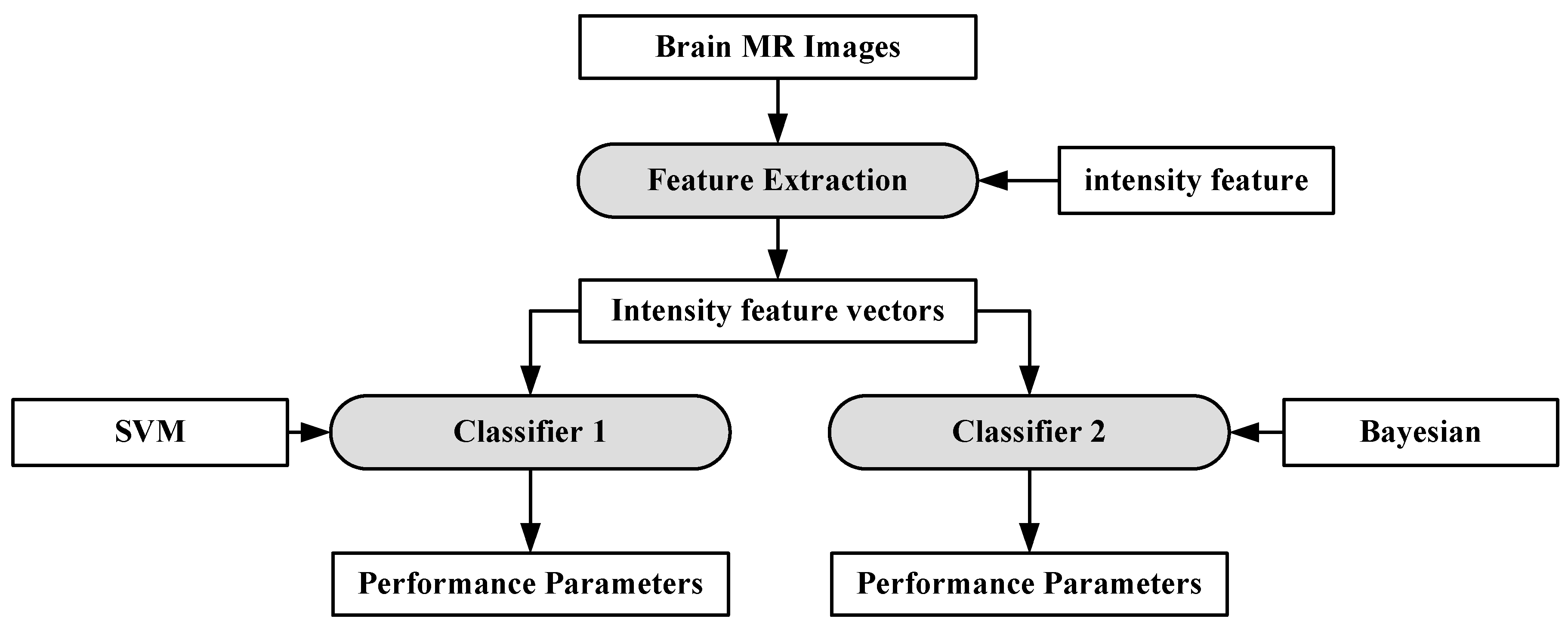
| 2 | Verma et al. 2008 [94] | Neoplasms, edema, and healthy tissue | DWI, B0, FLAIR, T1, and GAD | 14 (G-3 = 8, G-4 = 7) | Bayesian, and SVM | ACC = NA; SEN = 91.84; SPC = 99.57; AUC = NA | ||
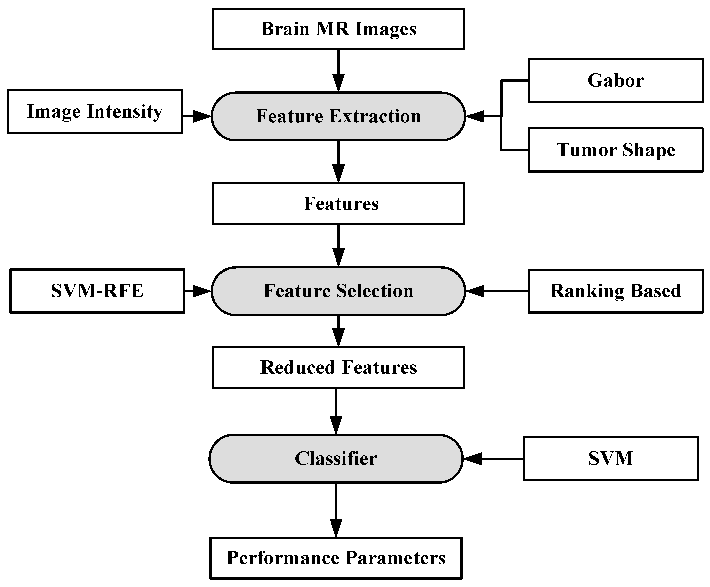
| 3 | Zacharaki et al. 2009 [92] | Metastasis, meningiomas gliomas (G-2-3) GBM | T1W, T2W, FLAIR, rCBV | 102 (Metastasis (24), meningiomas (4), gliomas (G-2) (22), gliomas (G-3) (18), GBM (34)) | SVM, RFE | Feature Ranking | LDA, KNN, NL-SVM | ACC = 97.8%; SEN = 100%; SPC = 95%; AUC = 98.6% |
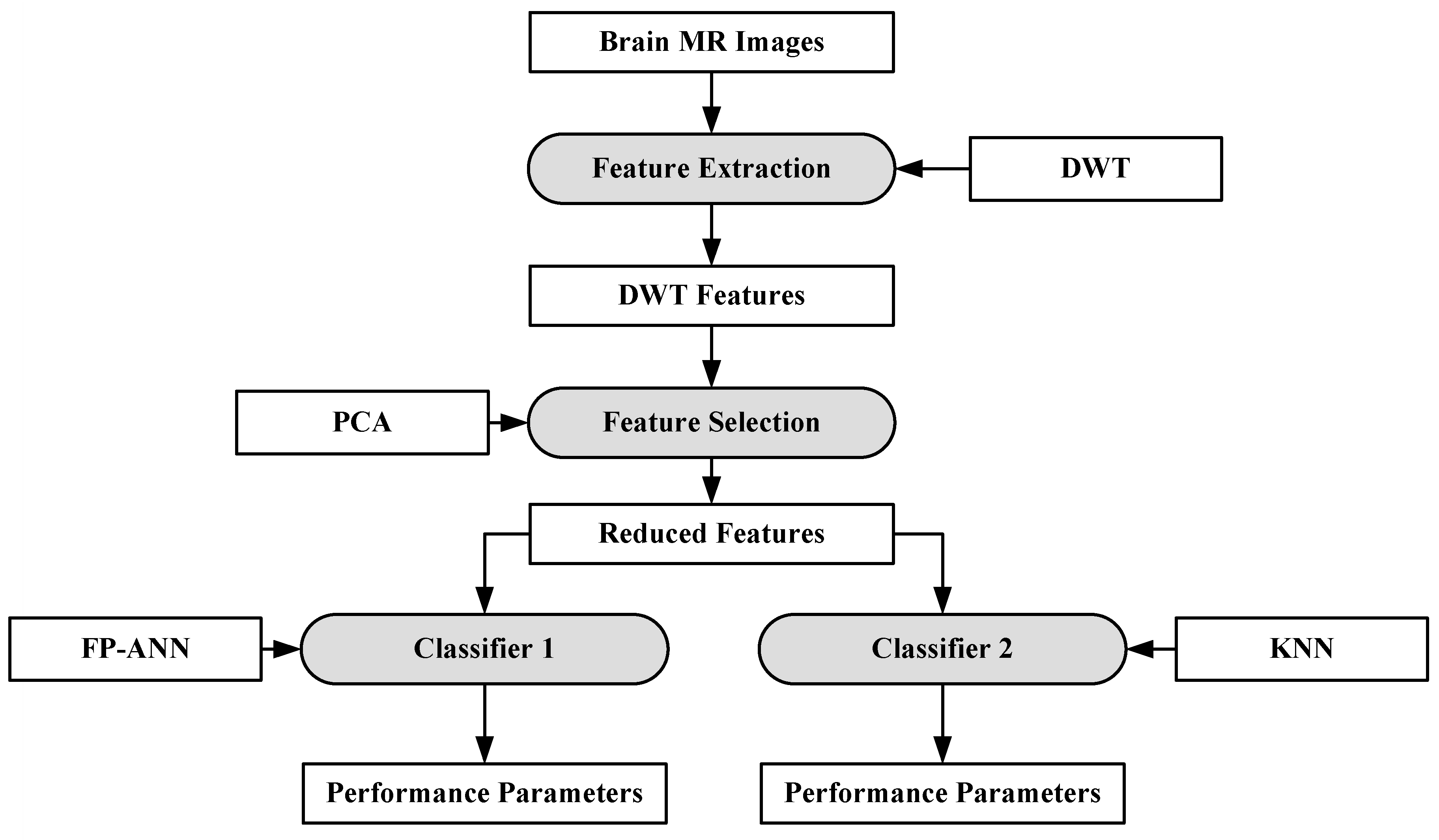
| 4 | El-Dahshan et al. 2010 [88] | N, ABN | T2W | 60, (N = 60, ABN = 10) | DWT | PCA | FP-ANN, KNN | ACC = 98.6%; SEN = 100; SPC = 90; AUC = NA |
| 5 | Ryu et al. 2014 [123] | Glioma (G-2,3,4) | DWI, ADC | 42 Glioma (G2(N = 8)), G-3 (N = 10) and G-4 (N = 22)) | GLCM | Entropy, Histogram | ACC = 84.4%; SEN = 81.8%; SPC = 90%; AUC = 94.1% | |
| 6 | Skogenet al. 2016 [105] | LGG (G-2), HGG (G-3-4) | T1W, T2W, FLAIR | 95 (LGG = 27 (G-2I) HGG = 68 (G-3 = 34 and G-4 = 34) | Statistical Analysis | Standard Deviation | ACC = 84.4%; SEN = 93%; SPC = 81%; AUC = 91% |
© 2019 by the authors. Licensee MDPI, Basel, Switzerland. This article is an open access article distributed under the terms and conditions of the Creative Commons Attribution (CC BY) license (http://creativecommons.org/licenses/by/4.0/).
Share and Cite
Tandel, G.S.; Biswas, M.; Kakde, O.G.; Tiwari, A.; Suri, H.S.; Turk, M.; Laird, J.R.; Asare, C.K.; Ankrah, A.A.; Khanna, N.N.; et al. A Review on a Deep Learning Perspective in Brain Cancer Classification. Cancers 2019, 11, 111. https://doi.org/10.3390/cancers11010111
Tandel GS, Biswas M, Kakde OG, Tiwari A, Suri HS, Turk M, Laird JR, Asare CK, Ankrah AA, Khanna NN, et al. A Review on a Deep Learning Perspective in Brain Cancer Classification. Cancers. 2019; 11(1):111. https://doi.org/10.3390/cancers11010111
Chicago/Turabian StyleTandel, Gopal S., Mainak Biswas, Omprakash G. Kakde, Ashish Tiwari, Harman S. Suri, Monica Turk, John R. Laird, Christopher K. Asare, Annabel A. Ankrah, N. N. Khanna, and et al. 2019. "A Review on a Deep Learning Perspective in Brain Cancer Classification" Cancers 11, no. 1: 111. https://doi.org/10.3390/cancers11010111