Article

WEBSEIDF: A Web-Based System for the Estimation of IDF Curves in Central Chile

by
Roberto Pizarro
1,
Ben Ingram
2,
Fernando Gonzalez-Leiva
1,
Rodrigo Valdés-Pineda
1,3,*,
Claudia Sangüesa
1,
Nicolás Delgado
1,
Pablo García-Chevesich
4,5 and
Juan B. Valdés
3
1
Technological Center for Environmental Hydrology, University of Talca, Talca, 3460000, Chile
2
School of Water, Energy and Environment, Cranfield University, College Rd, Cranfield MK43 0AL, UK
3
Department of Hydrology & Atmospheric Sciences, University of Arizona, Tucson, AZ 85721, USA
4
Faculty of Forest Sciences and Nature Conservation, University of Chile, Santiago 8320000, Chile
5
Department of Agricultural and Biosystems Engineering, University of Arizona, Tucson, AZ 85721, USA
*
Author to whom correspondence should be addressed.
Hydrology 2018, 5(3), 40; https://doi.org/10.3390/hydrology5030040
Submission received: 1 July 2018 / Revised: 27 July 2018 / Accepted: 2 August 2018 / Published: 4 August 2018

Abstract

:
The lack of reliable continuous rainfall records can exacerbate the negative impact of extreme storm events. The inability to describe the continuous characteristics of rainfall from storm events increases the likelihood that the design of hydraulic structures will be inadequate. To mitigate extreme storm impacts and improve water governance at the catchment scale, it is vital to improve the availability of data and the array of tools used to model and forecast hydrological processes. In this paper, we describe and discuss the implementation of a web-based system for the estimation of intensity–duration–frequency (IDF) curves (WEBSEIDF) in Chile. The web platform was constructed using records from 47 pluviographic gauges available in central Chile (30–40° S), with at least 15 years of reliable records. IDF curves can be generated for durations ranging from 15 min to 24 h. In addition, the extrapolation of rainfall intensity from pluviograph to pluviometric gauges (i.e., 24-h rainfall accumulation) can be carried out using the storm index (SI) method. IDF curves can also be generated for any spatial location within central Chile using the ordinary Kriging method. These procedures allow the generation of numerical and graphical displays of IDF curves, for any selected spatial location, and for any combination of probability distribution function (PDF), parameter estimation method, and type of IDF model. One of the major advantages of WEBSEIDF is the flexibility of its database, which can be easily modified and saved to generate IDF curves under user-defined scenarios, that is, changing climate conditions. The implementation and validation of WEBSEIDF serves as a decision support system, providing an important tool for improving the ability of the Chilean government to mitigate the impact of extreme hydrologic events in central Chile. The system is freely available for students, researchers, and other relevant professionals, to improve technical decisions of public and private institutions.

1. Introduction

Intensity–duration–frequency (IDF) curves are constructed based on the frequency of annual maximum rainfall intensities. They are an essential tool for the design of drainage and flood prevention infrastructures in urban areas. IDF curves ensure that hydraulic structures are adequate for, and can withstand the impacts of, extreme storm events, that is, that the collapse of drainage systems, damage to infrastructure, and loss of human life will not occur as the result of large floods, landslides, mudflows, and so on [1,2,3]. Extremes in the variability of the hydrologic cycle increase the negative effects of major storm events, because infrastructure design is less likely to be commensurate to the hydrologic effects of these storms [4,5]. Recent studies have used IDF curves to force hydrological models evaluating river basin responses for hydrologic design and water management [6,7,8,9].
As the probability of observing a greater frequency and intensity of storm events is expected to increase [10,11], the development of IDF curves will be a crucial challenge to minimize the vulnerability and exposure of ecosystems and human systems to the effects of global warming [12,13,14,15,16]. Research efforts have been focused on developing and evaluating IDF curves under non-stationary conditions (climate change scenarios), in order to establish differences between historical and future design storms [17,18,19,20,21]. However, in many places of the world, the inability to access data to evaluate mitigation and adaption options, and the lack of technical resources to implement adaptation options, have been identified as barriers to climate change adaptation [22,23]. The lack of consistent spatio-temporal distribution of ground-based rainfall intensity records is an additional challenge that governments and water resources managers face. To address this gap, web-based systems are a supportive tool aimed to storing and displaying historical and future projections of storm designs.
Central Chile (30–40° S), where 73% of the national population is concentrated [24], is cyclically impacted by extreme hydrological events. Precipitation along this Mediterranean territory is caused primarily by winter (austral) frontal systems [25,26,27,28,29]. These systems generate storms that can be similar in intensity to the convective systems registered in northern Chile [30]. It is estimated that the Chilean Government invested about US$1.5M to help with the recovery efforts derived from the damage caused by frontal precipitation systems that affected central Chile between 2000 and 2009 [31]. This magnitude of damages can be attributed to the lack of spatio-temporal hydrological information, the unplanned development activities by private and public entities, and the poor implementation of suitable policies for land management. In other words, the region is not well prepared to face the extreme events resulting from global warming [16].
Given the Chilean authorities’ interest on implementing a statistically reliable and robust system to store historic records of extreme storm events for central Chile, a web-based system for the generation of IDF curves (WEBSEIDF) was developed using rainfall intensity records from 47 pluviograph stations distributed in central Chile. WEBSEIDF makes it possible to construct IDF curves for durations of 0.25, 0.5, 0.75, 1, 4, 6, 12, and 24 h. The system also enables the extrapolation of IDF curves to ungauged areas, that is, in pluviometric gauges, IDF curves can be constructed using the storm index (SI) method, a linear scaling method proposed by the authors of [32]. A geostatistical method to extrapolate IDF curves has been also included in WEBSEIDF, that is, the ordinary Kriging method. This system provides a solution for ungauged areas that require the development of IDF curves for hydraulic structure design. Details about the structure and use of WEBSEIDF are provided in the following sections of this manuscript.

2. Methods

In this section, the procedures that were used to construct the IDF curves and their further integration into WEBSEIDF are described. Each of the sections that comprise the methodology is linked to the process of developing the database and the elements (user’s interface) that allow the user to interact with the tools in WEBSEIDF.

2.1. Intensity–Duration–Frequency Relationship

Precipitation, as a component of the water cycle, can be characterized based on three fundamental relationships: (1) the intensity, or temporal rate of precipitation (mm/h); (2) the duration for which the given average rainfall intensity will occur; and (3) the return period (T), which is the frequency or probability of occurrence [32,33,34]. The procedure to construct IDF curves is conducted by fitting rainfall intensity records to a probability density function (PDF), or a cumulative distribution function (CDF), while accounting for a specific duration that can vary from 15 min up to 24 h, as desired [34]. Annual maximum series (AMS) or partial duration series (PDS) can be used to construct the IDF Curves [19,35]. The maximum rainfall intensity for each duration is related to a return period (T), corresponding to a CDF. In terms of probability, T can be defined as a function of the probability of exceedance (occurrence) as follows:
P ( X > x T ) = 1 T   and   P ( X x T ) = 1 1 T
where,
  • P(X > xT) is the probability of exceedance within a year of a storm event with rainfall intensity xT.
  • P(X ≤ xT) is the probability of occurrence within a year of a storm event with rainfall intensity xT.
  • T is the return period or the number of years.
If the CDF is known, the frequency of extreme storms can be determined by fitting annual maximum rainfall intensity records to a PDF that best describes the temporal distribution of these independent events. According to the authors of [36], among all available PDFs, the most commonly used functions for describing random variables for maximum rainfall intensities are the following: generalized extreme value (GEV), Gumbel, and Pearson type-III. In WEBSEIDF, the user has the option to select some of the aforementioned PDFs to fit the historical intensity records, while accounting for different “goodness of fit” tests. Although this flexibility is available, it has been shown by the authors of [30] that the fit of the Gumbel distribution obtains good results in central Chile, where most pluviograph gauges are concentrated. Likewise, the Pearson-III PDF has demonstrated a good fit for data on arid and semi-arid regions of Chile (29–32° S), where rainfall intensity records have higher variability.

2.2. Probability Density Functions Included in WEBSEIDF

When annual maximum rainfall records are available, a frequency analysis can be conducted to estimate the exceedance probabilities, whose reciprocal is the return period [34,35,36]. Table 1 summarizes the PDFs implemented in WEBSEIDF. Further details related to the theory of frequency analysis in hydrology can be found in the literature [37,38,39,40,41,42]. The available PDFs in the WEBSEIDF system are considered sufficient for most modeling situations.

2.3. Parameter Estimation Methods

In hydrology, PDF parameters are usually estimated using the method of moments (MoM), which is simple and easy to implement. The maximum likelihood (ML) method is more complex due to the required algebraic manipulation [43,44], even though it can be very efficient when the sample size is large [45]. Greenwood [46] proposed another method to estimate parameters using probability weighted moments (PWM). One advantage of this method is that it can be written in an inverse form for Gumbel and Weibull; it also provides better results for the GEV in terms of bias and variance for sample sizes between 15 and 100 data points [44,47]. These advantages outweigh the fact that for small sample sizes, the ML can generate spurious values for the k parameter [48]. These three methods—MoM, ML, and PWM—have been implemented in WEBSEIDF and allow the user to compare the performance and results provided by the methods.

2.4. Mathematical Modelling of IDF Curves

Traditionally, IDF curves are represented graphically, which can introduce bias during the reading of a desired IDF curve. Interpretation errors are generally associated with the resolution of the printed curve on paper, and this error is amplified when the information is used for the design of hydraulic structures. Bernard [49] was one of the first to develop a mathematical model that describes rainfall intensity as a function of certain return period (T) and duration (D). This model is parametrized by simple linear regression and can produce a family of IDF curves, eliminating subjective reading errors. Currently, there is a large range of mathematical models for the generation of IDF curves, all with a similar structure to that of Bernard’s model [49]. The mathematical models for IDF curve estimation that are available in WEBSEIDF are listed on Table 2; while not exhaustive, they are considered sufficient for most modeling scenarios.

2.5. Goodness-of-Fit of PDFs and Mathematical Models

To verify the consistency between the rainfall records, the PDFs, and the IDF models, three goodness-of-fit tests are used: (1) the Mann–Whitney U test can be applied with the aim of determining if the two independent samples (observed and modeled rainfall intensity) come from the same population [53]; (2) the non-parametric Kolmogorov–Smirnov (K–S) test [54], which is important to determine the maximum deviation (theoretic and observed) of the modeled rainfall intensity; and (3) the coefficient of determination (R2), which is used to estimate the percentage of variance explained by the modeled rainfall intensity [55], which can be determined as a combination of any selected PDF and/or IDF model. Both the Mann–Whitney U and K–S tests can be evaluated by looking at their p-values under the module Statistics (see Section 3.4). In the K–S test, the null hypothesis regarding the distribution of rainfall intensity records is rejected if the test statistic, D (maximum difference between observed and estimated rainfall intensity), is greater than the critical value obtained from a table associated to a desired alpha value (see Table 1). The Mann–Whitney test is based on a comparison between each observation and each value estimated by the fitted PDF. If both series have the same median, then each observed rainfall value has an equal probability of being greater or smaller than each value estimated by the PDF. As it is also possible that two or more observations estimated from the PDF can be equal to the observed rainfall intensity value, U can be calculated by allocating half of the tie to the observed rainfall intensity records, and the other half to the estimated values. This can be done by using the normal approximation with an adjustment to the standard deviation (see Table 1). It is important to mention that all tests are calculated by comparing the rainfall intensity records of both observed and theoretical distributions for all durations and period returns (two column vectors). A summary of the three goodness-of-fit tests implemented in WEBSEIDF is presented in Table 3.

2.6. Extrapolation and Interpolation of IDF Curves

Most of the rain gauges in Chile measure rainfall accumulation every 24 h, limiting the capacity to construct IDF curves in areas lacking pluviograph gauges or tipping buckets that can provide rainfall accumulation for durations shorter than 24 h. In order to extend the spatial distribution of IDF curves to pluviometric gauges (24-h rainfall accumulation), extrapolation or interpolation methods can be applied. Two methods have been implemented in WEBSEIDF: (1) storm index; and (2) ordinary Kriging. Details about both methods are described below.

2.6.1. Storm Index Method

The storm index (SI), proposed by the authors of [32], was implemented in WEBSEIDF. SI is a dimensionless scaling ratio that can be calculated for any pluviographic gauge. This ratio is calculated between the maximum rainfall intensity in 24 h and the rainfall intensity for all durations less or equal than 24 h. Pizarro et al. [32] indicated that reliable constructions of IDF curves in pluviometric gauges are attained when the maximum absolute difference between the raw rainfall intensity in 24 h for both pluviographic and pluviometric gauges does not exceed 2 mm/h. The method assumes that rainfall characteristics observed in the pluviographic gauge are similar to those of the pluviometric gauge; however, this does not necessarily mean that the two gauges have to share similar climatic patterns. In fact, Pizarro et al. [30] concluded that maximum rainfall intensities values in Chile can be similar at different latitudes, that is, convective storms of northern Chile can be of similar intensity than frontal storms of central and southern Chile. The SI method was developed by [1] and validated for central Chile by [32]. The SI method is defined by the following expression:
S I ( i j ) = I max ( i j ) I max ( 24 , j )
where S I ( i j ) is the storm index in the pluviograph gauge for the duration i (hours), and the return period j (years); I max ( i j ) is the maximum rainfall intensity for the duration i and return period j; and I max ( 24 , j ) is the maximum rainfall intensity in 24 h for the return period j. This linear scaling method allows the increase of the spatial distribution of maximum rainfall intensity and the corresponding IDF curves, thus improving the availability of hydrological data for hydrologic design and water management. The WEBSEIDF also makes this method available so the user can spatially extrapolate rainfall intensity data (and IDF curves) to pluviometric gauges.

2.6.2. Ordinary Kriging

Geostatistical interpolation was also implemented in WEBSEIDF. Ordinary Kriging interpolation is used to reproduce a spatial prediction of rainfall intensity at any location of interest within the domain of interest. This method uses a semivariogram or a covariance model that relies on spatial relationships of rainfall intensity data [56,57]. The method is a geostatistical interpolation method similar to the inverse distance weighting (IDW) because it also weights nearby data points. In Kriging, however, the weights are not only dependent on distance; but they also depend on the overall spatial distribution of the data points. The method has been widely used in hydrology to determine spatio-temporal patterns of rainfall, and also in other environmental sciences [58,59,60]. The Kriging method is defined as a linear sum:
Z ^ ( S 0 ) = i = 1 N λ i Z ( S i )
where,
  • Z ( S i ) is the measured rainfall intensity value at the location i
  • λ i is the weight for the location i
  • S 0 is the predicted location
  • N is the number of measured values

2.7. Implementation and Validation of WEBSEIDF

WEBSEIDF offers a geographical information system (GIS) interface that enables users to easily access historical information from individual or multiple pluviograph gauges located in central Chile. Additionally, users provide updates to the database (in the necessary format) if newer data or gauges are needed to construct IDF curves. WEBSEIDF is similar in structure and components to the web tool developed and described by the authors of [23], for the generation of IDF curves under climate change scenarios in Canada. WEBSEIDF was developed in three stages: (1) collection of the rainfall intensity measurements database; (2) construction of IDF curves and mathematical models; and (3) development of a web-based GIS interface allowing simple browsing by users.

2.7.1. Consolidation of a Rainfall Intensity Database

To determine maximum rainfall intensities for durations between 1 and 24 h from pluviograph gauges, data from pluviograph strip charts must be analyzed (see details in [61]). However, there are limits to the usefulness of these data for durations of less than one hour. To overcome this problem, a device that uses an algorithm for automatic digitization of pluviograph strip charts was developed to calculate rainfall intensities for 15-min increments, ranging from 0.25 to 24 h (see details in Section 2.7.2). The device significantly improves the reading resolution of rainfall intensity records for the construction of IDF curves in Chile. It was initially used to estimate the rainfall intensity signals from the pluviograph strip charts kept by the National Directorate of Water Resources (DGA), the government organization responsible for monitoring and managing water resources in Chile. Additionally, data were digitized from pluviograph strip charts maintained by other water-related institutions, such as the Chilean Meteorological Directorate and the electric generation company ENEL (also known as ENDESA). After all data from the collected strip charts were digitized, a database containing 47 pluviograph gauges (see Appendix A) was consolidated, containing at least 15 years of rainfall intensity records. The established threshold allowed for the development of a database that can be considered statistically reliable, relative to the historical pluviograph records available in the country. Regarding the length of the rainfall series, it is important to mention that at least 30 years of records are needed to reduce the uncertainty of the rainfall estimates for T greater than 20 years. This is an advantage of WEBSEIDF because it allows the users to make updates in the spatio-temporal resolution of the database, that is, increase the number of gauges or add new records in existing gauges.

2.7.2. Pluviograph Strip Charts Reader

A device named a pluviograph strip charts reader (PSCR) was developed to digitize the analog pluviograph strip charts (manuscript under preparation). The PCSR significantly reduced the time to analyze a single pluviograph strip chart, because traditional time-consuming and error-prone manual techniques are replaced by a semi-automatic process of tracing the rainfall signal. The device was designed to read rainfall intensities in increments as small as 15 min, with a temporal displacement of 5 min; thus, the PCSR can generate a whole range of rainfall intensity durations. However, because of the thickness of the drawn trace in the pluviograph strip charts, rainfall intensity for durations of less than 15 min cannot be reliably extracted. In fact, reading tests show unreliable intensity readings at resolutions lower than 15 min. As a result, WEBSEIDF was implemented to provide the following durations: 0.25, 0.5, 0.75, 1, 2, 4, 8, 12, and 24 h. The configuration of PSCR has the following components: (1) processing server, (2) scanner, and (3) digitization software (Figure 1).
The software used in PSCR is web-based and server-stored. It enables the simultaneous analysis of pluviograph strip charts via wireless connection, for up to five end users, without affecting the computational efficiency. This capability means a considerable reduction in processing time, as well as an increased capacity for extracting and managing large volumes of data. The PSCR uses a scanner to extract the rainfall intensity data, taking into consideration the need to acquire images from pluviograph bands of the size 9 × 42.5 cm. The scanner is an Epson Workforce Pro GT-S50, with automatic sheet feeder, able to read 50 double-sided sheets per minute. Given the size of the charts, the scanner was configured to capture images at a resolution of 5019 × 1181 pixels and 300 dots per inch (dpi).
Using the algorithm designed for the automatic digitization of strip charts, the PSCR automatically generates a trace of the rainfall intensity signal that is overlaid on the scanned image. This trace can be adjusted by the end user to correct possible errors derived from handwritten annotations, which are very common and can reduce the effectiveness of the algorithm. Once the band trace has been completed, rainfall intensity time series can be extracted as a plain text file, which can then be used to calculate annual maximum rainfall intensities. As a validation procedure, the digitized rainfall intensity data obtained from PSCR for durations of 1, 6, and 24 h were compared to manually extracted data for the same durations. For all analyzed cases, the Mann–Whitney U test confirmed that there were no statistically significant differences (α-level or significance level of 0.05) in the calculated values of rainfall intensity.

2.7.3. Database for Mathematical Models

Each of the mathematical models was developed in Python using the methods described in Section 2.4, and then implemented in WEBSEIDF. The modelling process is conducted in two stages: (1) a PDF (see Table 1) is fitted to the annual maximum rainfall intensities associated with each duration (D) and return period (T), and (2) an analysis using ordinary least squares regression (OLSR) was conducted to estimate the optimal parameters for all the models presented in Table 2 [62]. The performance of the models is evaluated using the tests described in Table 3. Additionally, a geostatistical tool that uses ordinary Kriging [63] was also built-in to perform spatial interpolations and create isolines of maximum rainfall intensities within central Chile.

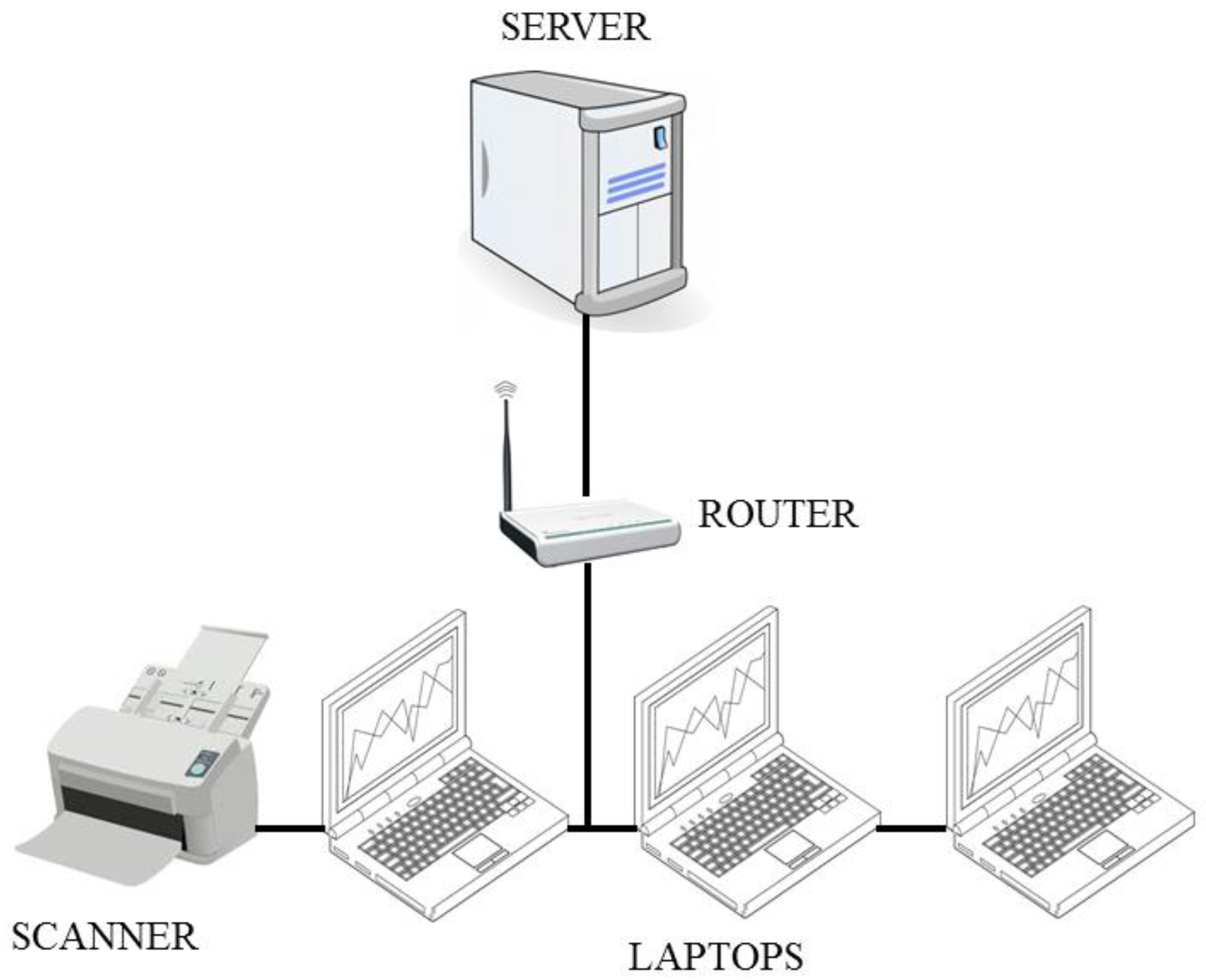
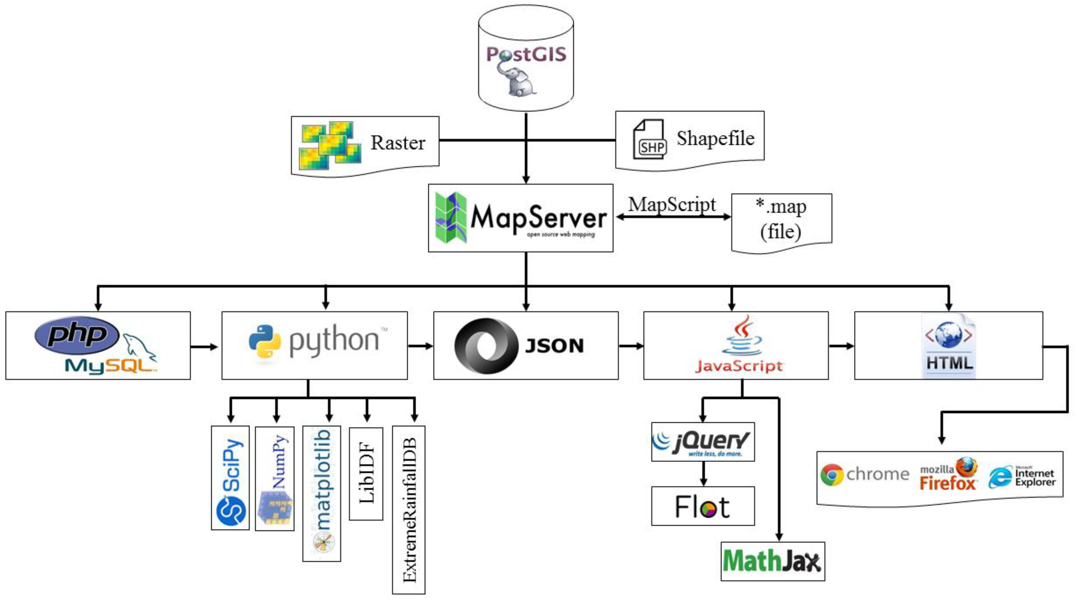
2.7.4. Informatic Development of WEBSEIDF

The development of WEBSEIDF responded to the need of an easily accessed database for rainfall intensity data extracted from pluviograph strip charts. In fact, WEBSEIDF is the first web-based system for IDF curves in Chile, and there are no similar systems available. WEBSEIDF is an innovative tool for storing, visualizing, and analyzing rainfall intensity data. The system required the addition of a spatial support component; PostGIS, which is an extension of the popular PostgreSQL, was used. A PHP (hypertext preprocessor) was used to connect directly to the database to visualize, modify, and register data supplied by the user and the stations that contain information about maximum rainfall intensities. A connection between Python and the database was established so that all mathematical operations and statistical analyses described in Section 2, Section 2.1, Section 2.2, Section 2.3, Section 2.4, Section 2.5 and Section 2.6 could be performed. The libraries NumPy, SciPy, and MatPlotLib were used. The results of the calculations were formatted using JSON, read using JavaScript, and finally visualized on a web page using HTML (v4). JavaScript libraries such as Flot were used to visualize the IDF curves. To generate the equations related to the IDF curves, LaTeX and MathML were used by the libraries JQuery and MathJax. For the graphical user interface (GUI), the Mapserver tool was used to create map visualizations displaying the available pluviograph gauges and rain gauges. Finally, WEBSEIDF was developed for common browsers including Internet Explorer, Mozilla Firefox, and Google Chrome (see Figure 2 for details). All software and informatics steps performed to develop WEBSEIDF are similar to those used by the authors of [23], in the development of a web-based tool for IDF curves estimation under climate change scenarios in Canada.
Some of the important advantages of WEBSEIDF are the following:
  • The system is web-based, allowing users to access it from any location with an Internet connection.
  • Its GIS-based architecture allows the integration of hardware, software, and georeferenced data in the process of capture, storage, manipulation, analysis, and visualization.
  • Its flexibility allows users to easily incorporate additional spatial data into the system—that is, the database allows the addition of new pluviograph gauges.
  • It is flexible enough to incorporate new processing algorithms and models to represent IDF curves.
The architecture and functionality of WEBSEIDF, which are linked to a GIS component, require the integration of different programming languages—that is, those used for mathematical calculations, and those used for management of the database. This system is designed to enable continuous development and improvement, to ensure current and future relevance to the management of water resources in central Chile.

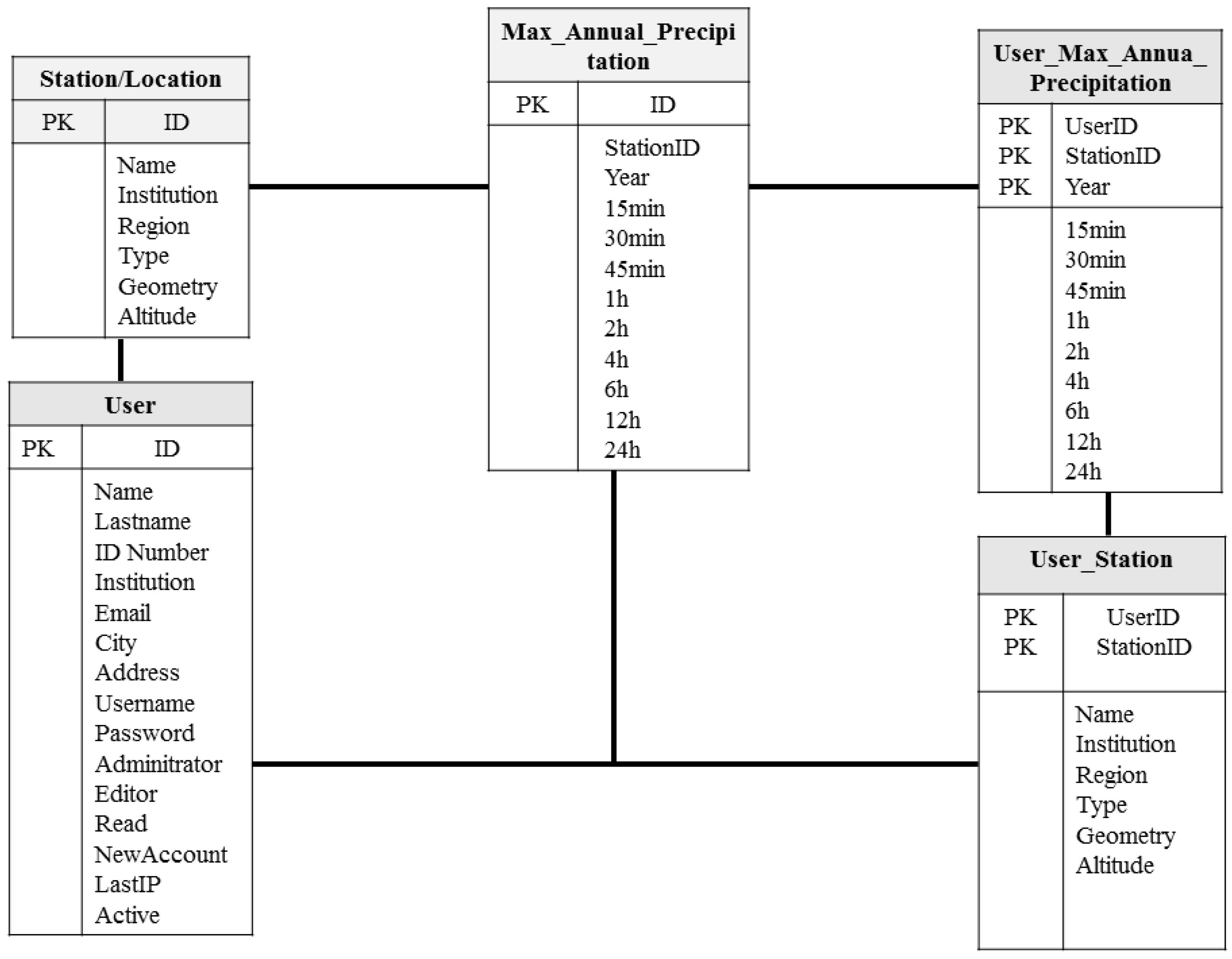
2.7.5. Georeferenced Database

The georeferenced database (geodatabase) for WEBSEIDF was designed to store, organize, and manipulate rainfall intensity data. The geodatabase design accounted for the following entities: (1) Users, which contains the list of users registered in the system; (2) Station, which stores the data from each pluviograph gauge or rain gauge; (3) User_Station, which stores the user’s data related to station data; (4) Maximum_Yearly_Precipitation, which contains the precipitation data from the pluviograph gauges or rain gauges; and (5) Users_Maximum_Yearly_Precipitation, which is a copy of the data provided in (4), allowing each user to have their own copy of the data (see Figure 3 for details).

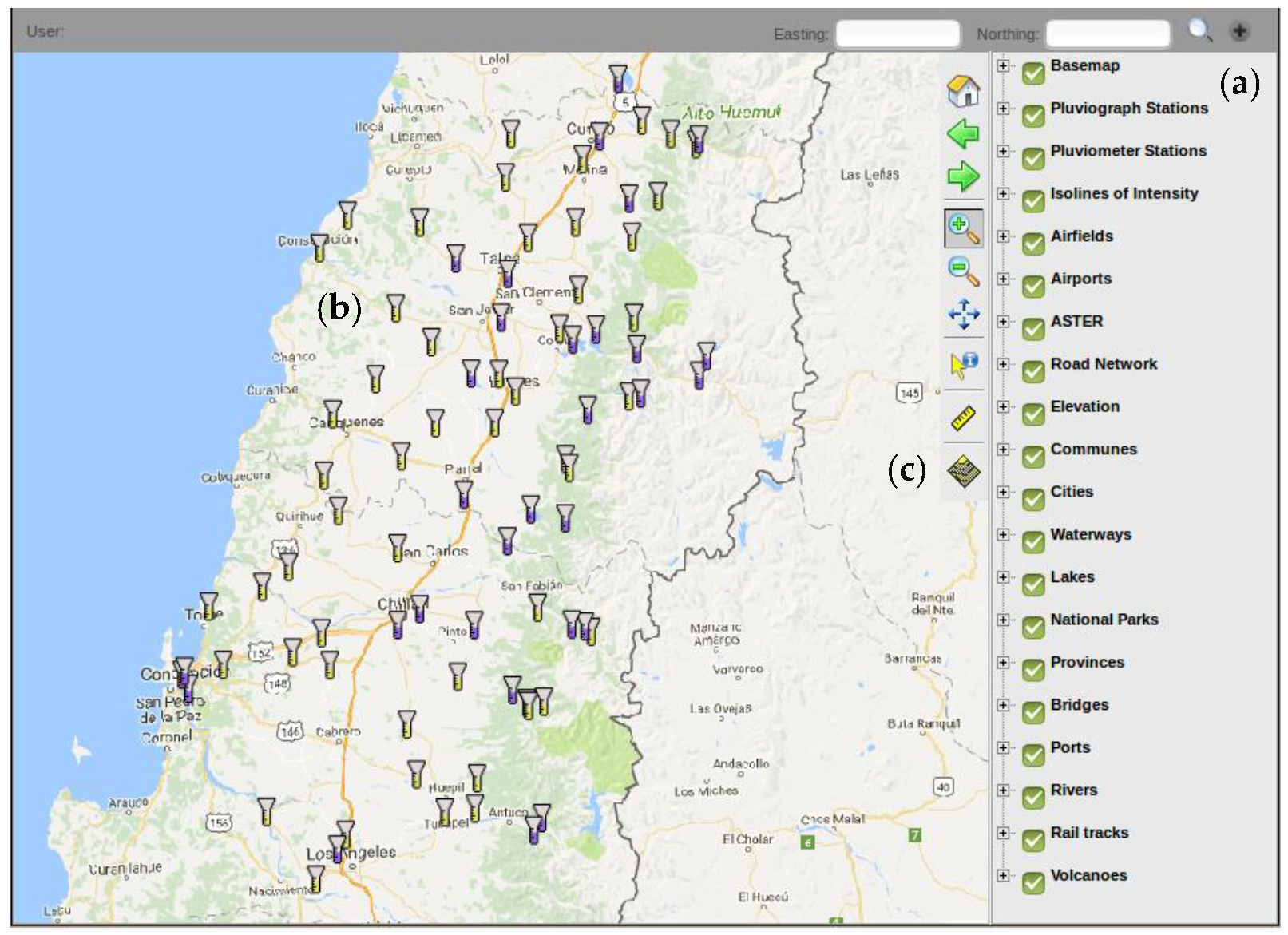
2.7.6. Graphical User’s Interface (GUI) of WEBSEIDF

The WEBSEIDF interface has an intuitive structure that allows users to easily explore all the tools available in the system. In fact, the GUI (graphical user interface) enables users to interact with available data and to generate the visualization of IDF curves and their mathematical models. The structure of the interface (Figure 4) is composed of the following elements: (a) a geographical information system (GIS) with a drop-down menu that contains satellite maps, cartographic information—that is, water resources, road networks, administrative divisions, and so on; (b) a georeferenced pluviographic and pluviometric gauges; (c) a toolbar menu that the user can use to manipulate the visualization in the GIS environment; and a control panel that allows administrative control of access privileges.

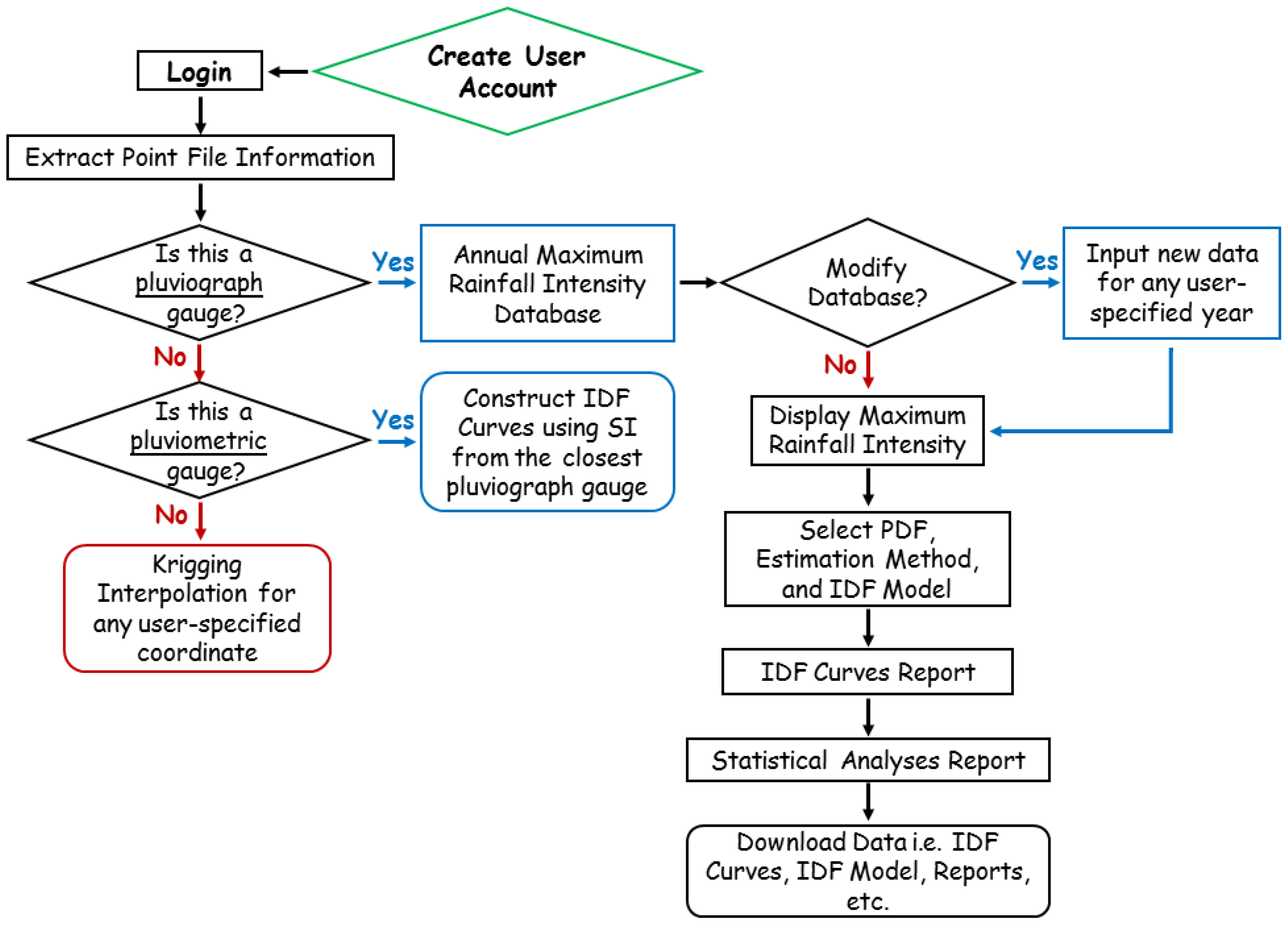
2.7.7. Procedure to Generate IDF Curves Using WEBSEIDF

The generation of IDF curves in WEBSEIDF is a straightforward procedure. First, a user account must be created, a process described in Section 3.1. WEBSEIDF contains a point-based database for central Chile that can be accessed, extracted, modified, and analyzed. This database has pluviograph and pluviometric gauges that can be used to generate IDF curves. For ungauged areas, the ordinary Kriging interpolation method allows for the construction of IDF curves at any spatial location within central Chile. In pluviometric gauges (24-h rainfall accumulation), the SI method is used to generate the IDF curves. Users can select from a complete set of PDFs, estimation methods, and IDF models to analyze and compare the sensitivity of the generated IDF curves. The flexibility of WEBSEIDF allows users to save modifications made to the database without affecting the records contained in the original database. This option is very useful for generating climate change scenarios based on modified rainfall intensity records [23]. These steps are summarized in Figure 5.

2.7.8. Considerations about the Methodologies Included in WEBSEIDF

The selection and compilation of storm records can include PDS or AMS. In general, PDS for frequency analysis can generate higher values for a given frequency, compared with AMS. The difference in rainfall intensity values is generally greater for the most frequent events (i.e., 2-year, 5-year, 10-year), and it decreases as the return period increases, that is, the difference in rainfall intensity values is minimal for less frequent events (i.e., 25-year, 50-year, 100-year, 500-year). The selection of either PDS or AMS can have significant implications in the design or control of drainage and flood prevention infrastructures [64,65]. Accordingly, it is recommended to test both types of series (with different PDFs and IDF models) to select the most appropriate model for the management of extreme hydrological events.
Regarding the ordinary Kriging method of interpolation included in WEBSEIDF, it is worth mentioning that this is just one of many techniques that can be used for the interpolation of spatial data. The basic assumption of Kriging is the principle that data spatially closer are more likely to be more similar in behavior than data with a larger separation distance. Although this assumption largely holds for climate data, there are other factors that determine rainfall intensities such as elevation and proximity to large bodies of water. Although techniques such as co-Kriging or regression Kriging can be used to model secondary variables, the ordinary Kriging method implemented in the WEBSEIDF system does not take this data into account, although currently, active research is being carried out to determine how best to model these and other secondary variables. Furthermore, another simplification introduced into the WEBSEIDF system is that users cannot estimate the covariance structure of the data. The covariance structure of the rainfall data was previously analyzed and determined and hence the covariance parameters have been fixed. As many users of the system may not be familiar with geostatistical methods and the associated parameter estimation stage, it was decided to fix these, which also ensures the stability of the Kriging process. When adding data from other spatial locations where rainfall characteristics maybe significantly different to the target area in south-central Chile, it will be necessary to reestimate these parameters.

3. Results and Discussion

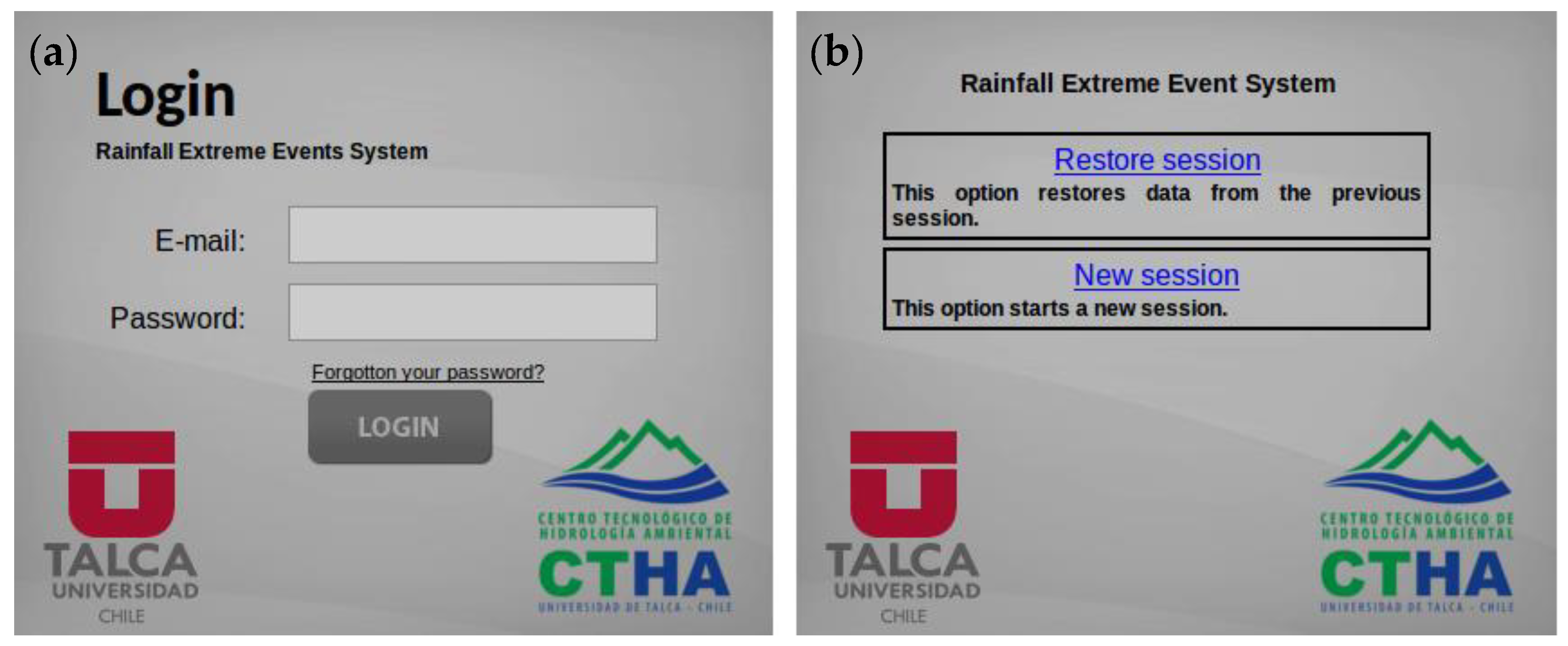
3.1. Register, Login, and Use of WEBSEIDF

WEBSEIDF is currently hosted on a server at the University of Talca, and can be accessed through the following link: http://ree.ctha.cl (or http://see.utalca.cl for spanish version). The system is able to store information from the end users to facilitate analysis about its usage. The conditions about usage and privacy policies have been established according to confidentiality policies. Once a user’s account has been created, their username and password are directed to a new window (Figure 6a) where it is possible to login into WEBSEIDF. In the next window, users can either start a new session or continue from a previous saved session, allowing them to make changes to the database and save these changes for future use (Figure 6b).

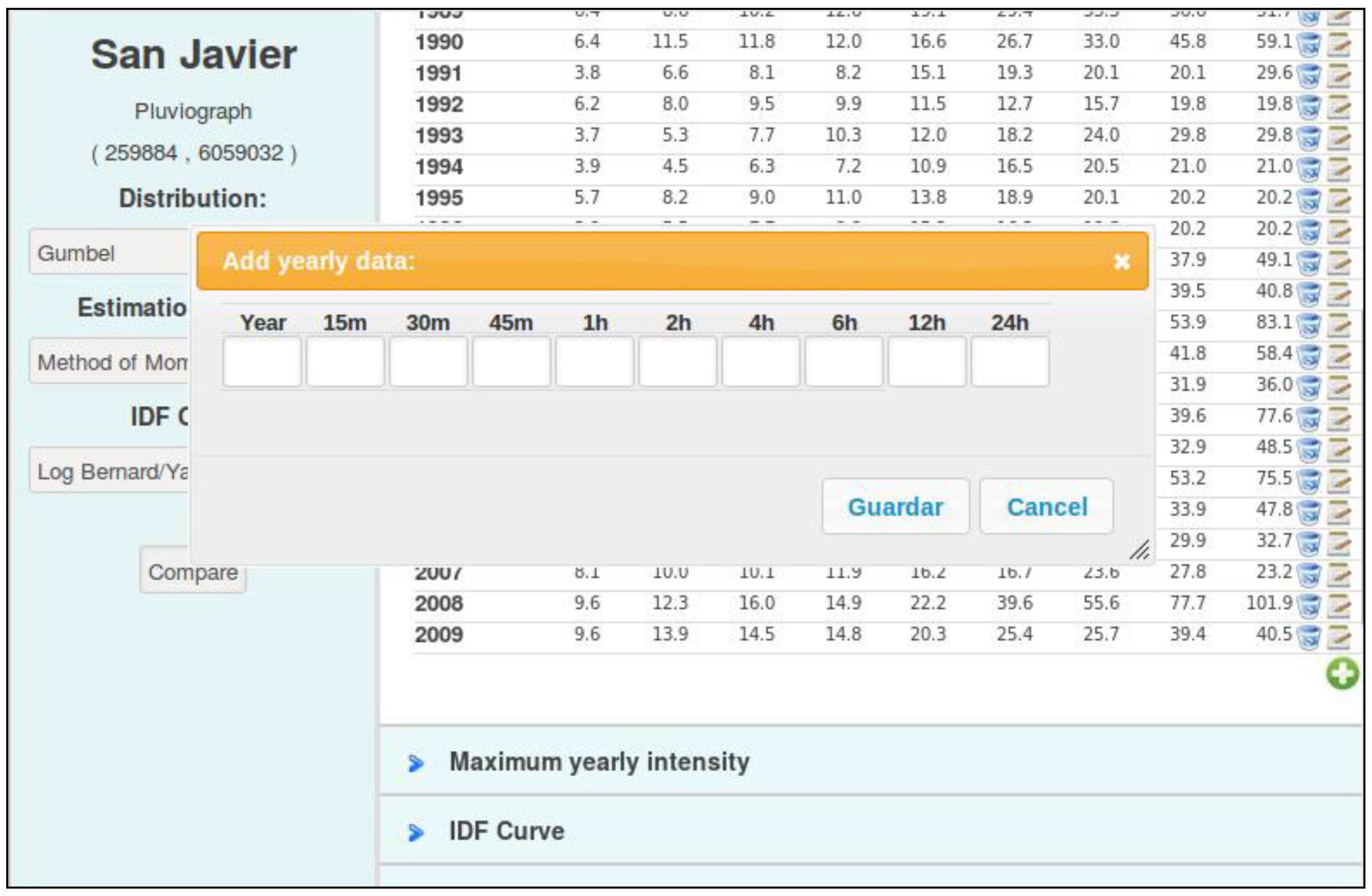
3.2. Spatial Visualization and Adding New Data into WEBSEIDF

To visualize or analyze rainfall intensity data in WEBSEIDF, users can generate queries by selecting a point-based feature (pluviograph gauge or rain gauge), or by entering the coordinates of the area of interest within central Chile (all available point-based features would be included inside this polygonal domain). For instance, if the user selects a single pluviographic gauge or pluviometric gauge (rain gauge), or clicks on the map, a new window providing specific information about the selected feature(s) opens up. The menu for this window allows selection of the PDF, the parameter estimation method, and the IDF model for each selected pluviographic gauge or pluviometric gauge. Once this information is selected, the user can visualize and export the following data and results: (1) annual maximum precipitation accumulation for different durations; (2) annual maximum rainfall intensity for different durations; (3) IDF curves; (4) mathematical models; (5) storm index; (6) statistics; (7) export; and (8) other associated analysis (Figure 7).
For any pluviographic gauge or rain gauge, it is possible to add new data—that is, information on maximum storm precipitation accumulation from newly acquired years. These data must be inputted for the entire range of durations established in WEBSEIDF, that is, 0.25, 0.5, 0.75, 1, 2, 4, 8, 12, and 24 h (see Figure 8), by an operator. Administrative privileges are required for users to be able to add new data to WEBSEIDF.

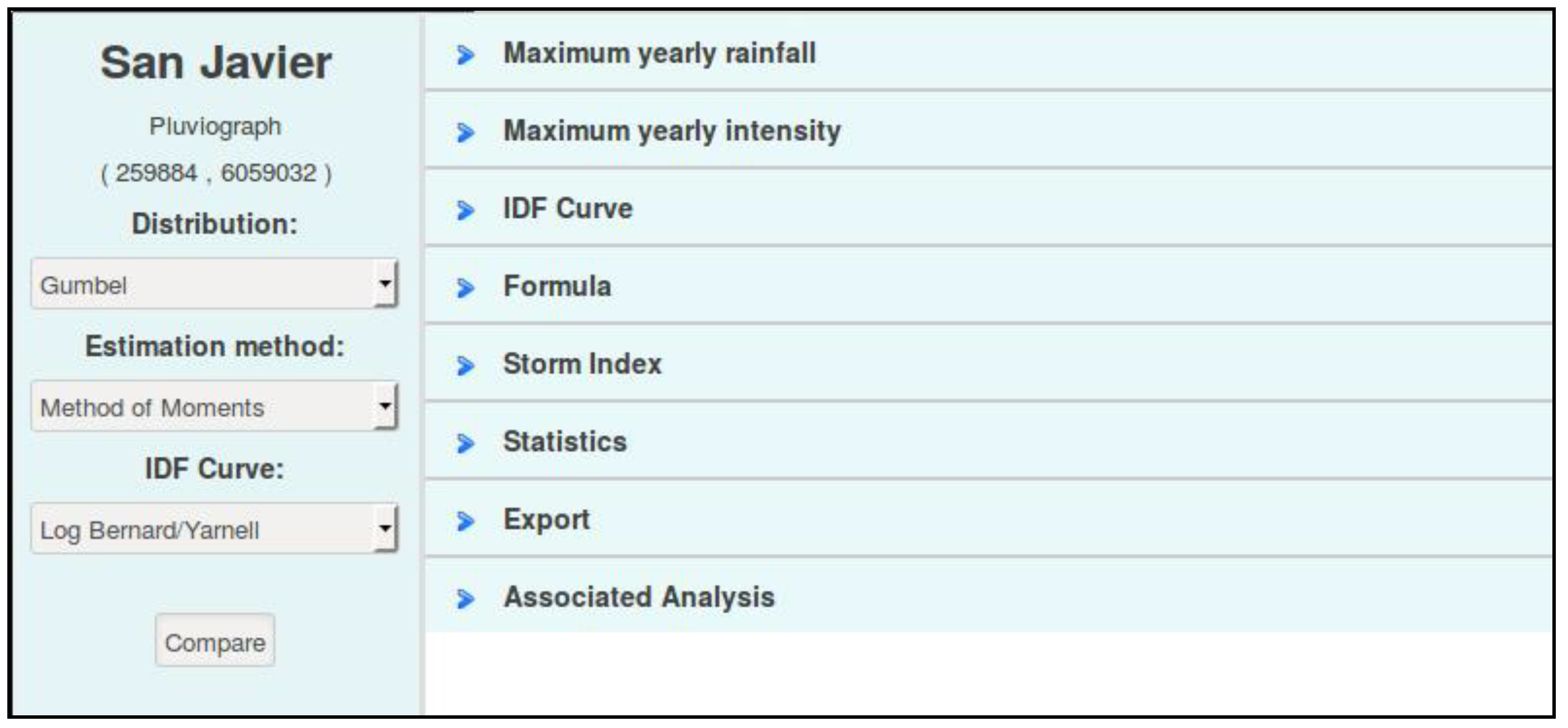
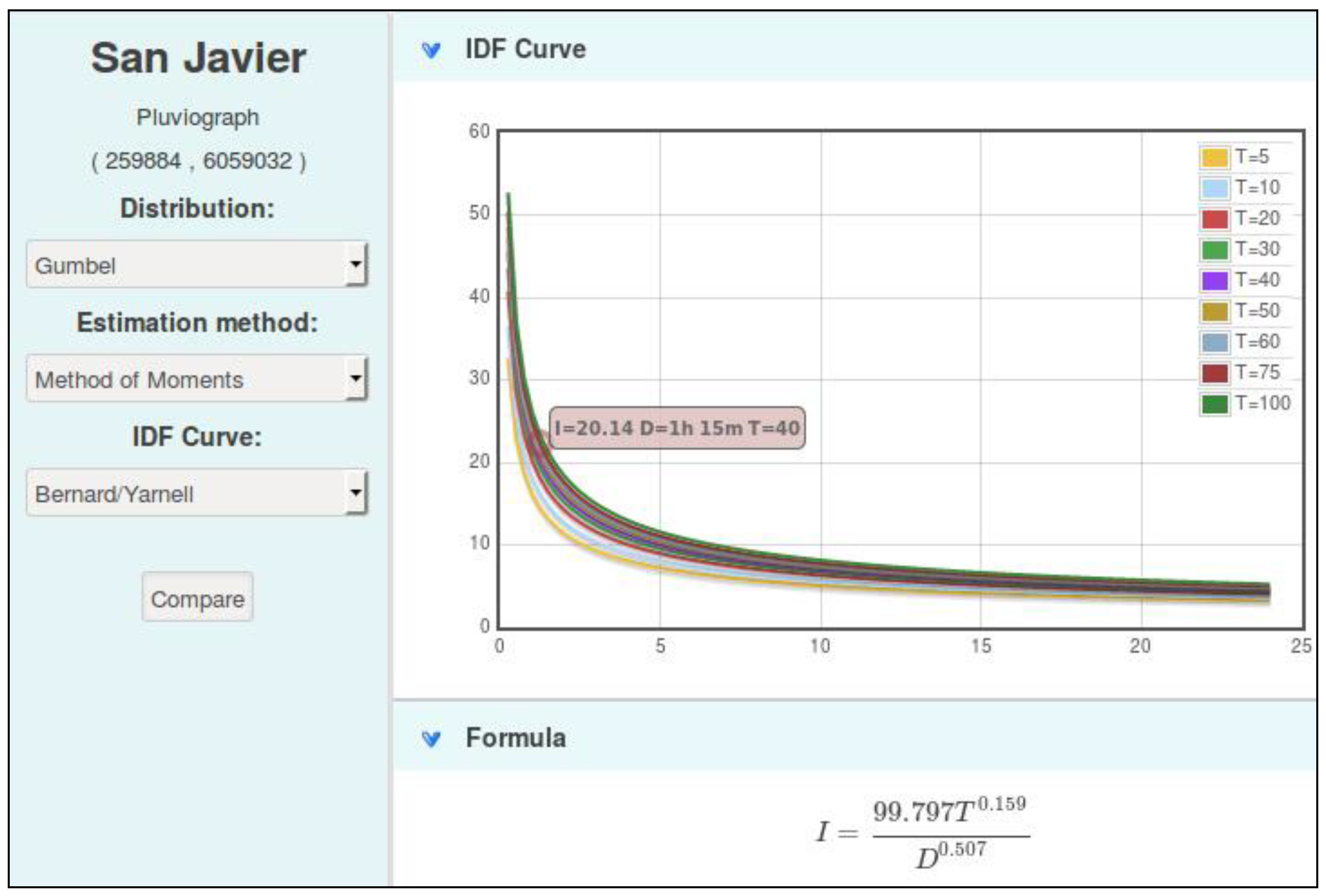
3.3. Graphical Visualization of IDF Curves

The annual maximum rainfall accumulation for a selected pluviograph gauge or rain gauge is converted into annual maximum intensities for the whole range of durations established in WEBSEIDF. This conversion provides data suitable for the estimation of IDF curves. In the current version of WEBSEIDF, the users can select any of the three available PDFs, the method for parameter estimation, and the IDF model to be fitted using the original rainfall intensity data. After selecting this primary information, the user can obtain a graphic representation of the IDF curves and the selected IDF model with its corresponding parameter values. The system allows positioning the mouse over any IDF curve to get a pop-up window showing the intensity of rainfall, the duration, and the corresponding return period. This is a handy option to easily display and determine rainfall intensity values along the IDF curves (see Figure 9). To determine the best fit for combinations of selected PDF and IDF models, the results of the fitted PDFs and mathematical models can be displayed in the Statistics module, which provides the results of three goodness of fit tests included in WEBSEIDF: Mann–Whitney, Kolmogorov–Smirnov, and coefficient of determination (see Section 2.5 and Figure 10 for details).

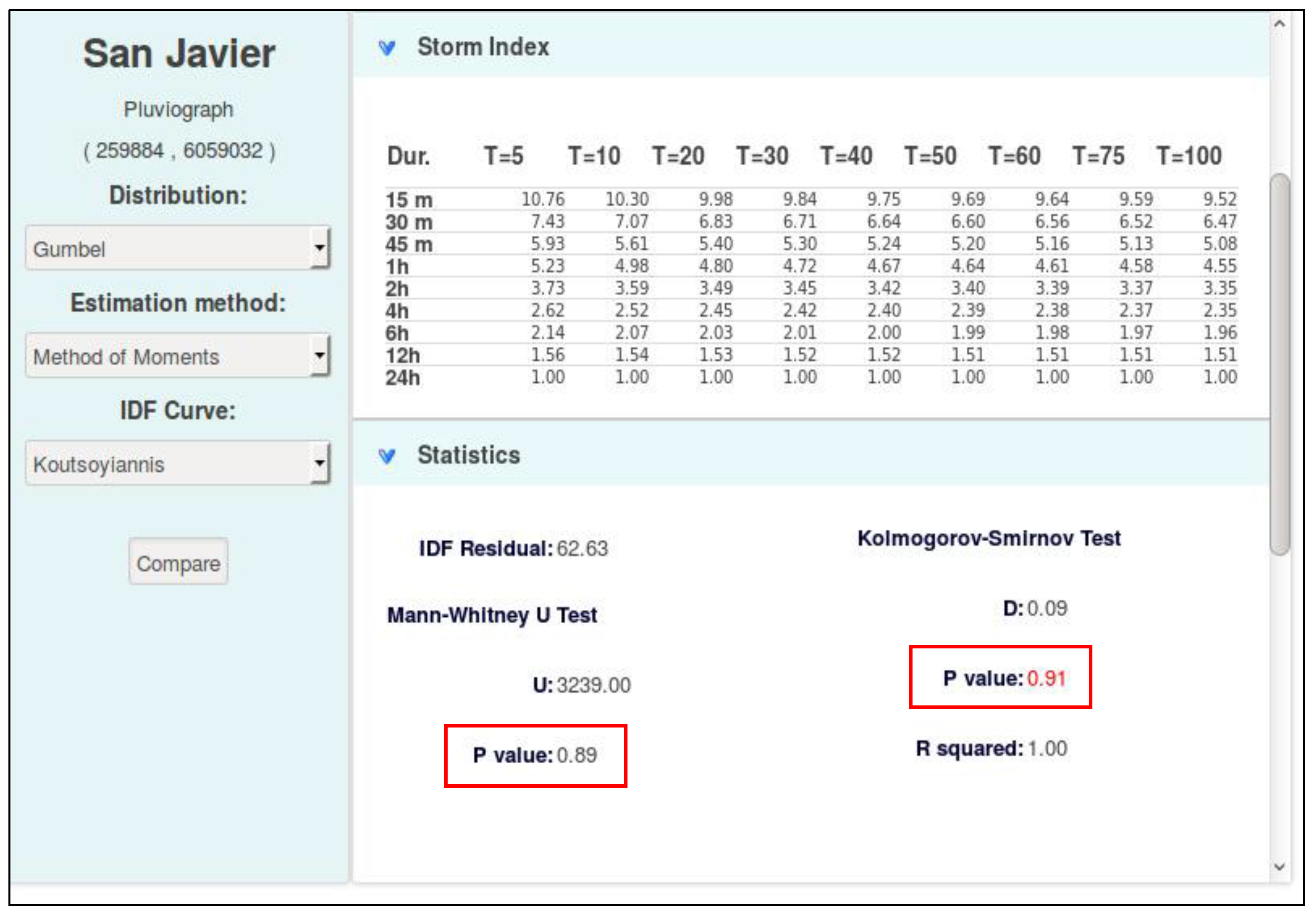
3.4. Extrapolation of IDF Curves

To extend the spatial distribution of IDF curves to pluviometric gauges (24-h rainfall accumulation), the storm index (SI) method [32] was implemented in WEBSEIDF. Users can construct IDF curves for the pluviometric gauges using the SI of a reference pluviograph gauge. As a reasonable rule of thumb, Pizarro et al. (2015) [32] suggested that consistent extrapolations of IDF curves are attained when the maximum absolute difference between the raw rainfall intensity in 24 h for both pluviographic and pluviometric gauges does not exceed 2 mm/h. In WEBSEIDF the SI is first calculated in a reference pluviographic gauge, and then used to generate IDF curves, their mathematical models, and statistics of interest for any neighboring pluviometric gauge. WEBSEIDF also allows the users to download .xls and .pdf formats of the raw data and IDF curves. More details about the options available in WEBSEIDF can be obtained from the user’s manual.

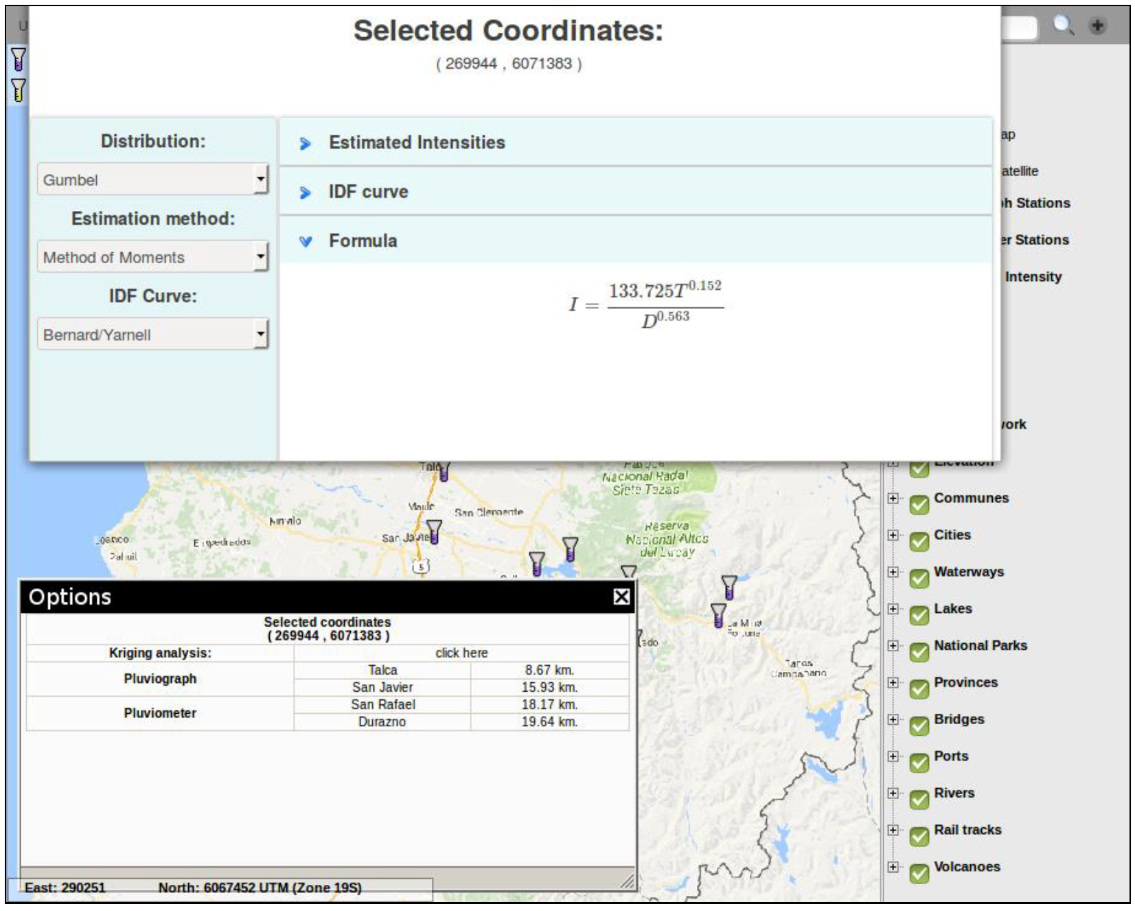
3.5. Geostatistical Interpolation of IDF Curves

Geostatistical interpolation of maximum rainfall intensities at specific user-defined locations is also available in WEBSEIDF. The system uses ordinary Kriging interpolation to reproduce a spatial prediction of IDF curves at any location of interest within central Chile. Available in the main interface toolbar, the interpolation option can be applied by selecting any spatial location or geographic point where the IDF curves need to be interpolated (Figure 11). The interpolation can be also applied for any selected pluviographic or pluviometric gauge. Once the user selects a point of interest (gauge), a report is displayed indicating the coordinates of the selected location, and the distance in kilometers from the nearest pluviograph and pluviometric gauges.

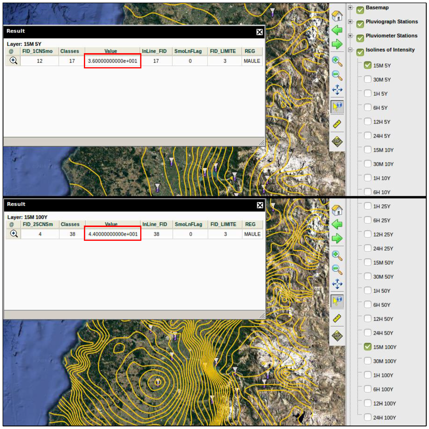
3.6. Isolines of Maximum Rainfall Intensity

This option allows generating isolines for the maximum rainfall intensity, considering all the pluviographic and pluviometric records available in central Chile. This choice can be accessed from WEBSEIDF drop-down menu. Activating this preference deploys isolines in the map for any selected duration and return period (Figure 12a,b). The rainfall intensity value (mm/h) contained in the isolines map can be displayed by positioning the identification tool (from the toolbar menu) over any desired spatial location. This selection allows for the visualization of the spatial distribution of maximum rainfall intensity records in central Chile, and the differences associated with the whole range of durations and return periods. The isolines of maximum rainfall intensity for any duration and return period are plotted considering all the available records available in WEBSEIDF database. The rainfall intensity value of any selected isoline is automatically displayed in a new window (see Figure 12).

4. Conclusions

WEBSEIDF is a web-based system that has been developed to consolidate a database of historical rainfall intensity records for central Chile. The system stores, visualizes, and analyzes maximum rainfall intensity records between 15 min and 24 h from pluviographic or pluviometric gauges, to generate IDF curves at any spatial location within the domain of central Chile. This is the first system capable of generating this level of spatio-temporal resolution in the development of IDF curves in central Chile. This innovation is very important because extreme rainfall events of shorter durations have often proven to be more powerful and destructive than those of longer duration. Additionally, the IDF curves can be extrapolated to ungauged areas (i.e., pluviometric gauges) using rainfall intensity data from pluviographs combined with the SI scaling method. WEBSEIDF also makes it possible to generate IDF curves for ungauged areas by interpolating data of existent pluviograph gauges. This approach to generate IDF curves has a substantial advantage, compared with methodologies such as generalized IDF curves, because it allows for the disaggregation of data on the spatial variability of rainfall intensity to a higher spatial resolution. Finally, it is important to point out that one of the major advantages of WEBSEIDF is the flexibility that allow users to add new rainfall intensity records into the database. WEBSEIDF is freely available for students, researchers, and other relevant professionals, providing capabilities that can be used to improve technical decisions of public and private institutions. The database provided by WEBSEIDF can be used in the design of major and minor storm water management systems, sanitary sewers, retention ponds, culverts, bridges, dams, pumping stations, roads, and drainage planning, and so on, to mitigate the impacts of extreme events in central Chile.

Author Contributions

Conceptualization, B.I. and N.D.; Funding acquisition, R.P., and C.S.; Investigation, R.P., B.I., R.V.P. and N.D.; Methodology, R.P., R.V.P., and F.G.L.; Project administration, R.P., and C.S.; Software, B.I., and N.D.; Writing—original draft, F.G.L., and R.V.P.; Writing—review & editing, R.P., B.I., F.G.I., R.V.P., P.G.-C. and J.B.V.

Funding

The paper was funded by the Chilean National Commission of Science and Technology (CONICYT) in the context of the project: “Estimation system of extreme rainfall events, for prevention and mitigation of stream flow and flood risks, in a variability and climate change context” (in Spanish), FONDEF-D08I1054.

Acknowledgments

WEBSEIDF was developed and implemented within the context of the project: “Estimation system of extreme rainfall events, for prevention and mitigation of stream flow and flood risks, in a variability and climate change context” (in Spanish), FONDEF-D08I1054. The pluviograph strip charts and the rainfall records used in WEBSEIDF were provided by the General Directorate of Water Resources (DGA), the Meteorological Directorate, and the Electric Generation Company (ENEL). All these contributions are gratefully acknowledged.

Conflicts of Interest

The authors declare no conflict of interest.

Abbreviations

IDFIntensity–Duration–Frequency Curves
WEBSEIDFWeb-based System for the Estimation of IDF Curves
SIStorm Index Method
PDProbability Density Function
CDCumulative Distribution Function
AMAnnual Maximum Series
PDPartial Duration Series
TReturn Period
DStorm Duration
GEVGeneralized Extreme Value
MoMMethod of Moments
MLMaximum Likelihood Method
PWMProbability Weighted Moments
K–S testKolmogorov–Smirnov Test
IDWInverse Distance Weighting
PSCRPluviograph Strip Charts Reader
DGADirección General de Aguas
ENELEnel Distribución Chile S.A.
DMCDirección Meteorológica de Chile

Appendix A

Table A1. Pluviograph gauges included in WEBSEIDF. The pluviographs bands were contributed by three Intitutions: The National Directorate of Water Resources (DGA), The National Company of Electricity (ENEL), and the National Meteorological Directorate (DMC).
OriginNameLat (S)Long (W)Period of RecordsAvailable Years
DGAEmbalse Rungue33°01′70°55′1979–200726
DGACerro Calán33°23′70°32′1975–201238
DGALos Panguiles33°26′71°00′1981–201131
DGAPirque33°40′70°36′1972–201039
DGAMelipilla33°40′71°11′1975–201237
DGALa Obra33°35′70°29′1995–201218
DGAHuechun Andina33°04′70°46′1994–201215
DGASan Antonio33°34′71°37′1997–201115
DGAMOP-DGA33°2670°38′1992–200817
DMCTobalaba33°27′70°32′1998–200912
ENELQuinta Normal33°26′70°40′1917–200989
ENELCerrillos33°29′70°42′1960–200545
ENELPudahuel DMC33°23′70°47′1974–200936
ENELEdificio Central Endesa33°27′70°39′1969–200123
DGALos Queñes35°00′70°49′1974–200936
DGAPotrero Grande35°12′71°07′1971–200938
DGAPencahue35°23′71°48′1974–200936
DGATalca35°26′71°35′1982–200928
DGASan Javier35°36′71°44′1974–200936
DGAColorado35°38′71°16′1969–200940
DGAMelozal35°45′71°47′1971–200935
DGAEmbalse Ancoa35°54′71°17′1971–200938
DGAParral36°09′71°50′1974–200936
DGAEmbalse Digua36°15′71°32′1971–200939
DGAEmbalse Bullileo36°17′71°26′1971–200939
DGASan Manuel36°21′71°39′1995–200915
DMCCurico34°57′71°13′1966–200940
ENELArmerillo35°42′71°06′1959–200041
ENELCasa de Maq. Cipreses35°48′70°49′1964–200030
ENELDesague Laguna Invernada35°44′70°47′1963–198018
ENELMelado en la Lancha35°51′71°04′1966–199325
ENELEl Lirio35°40′71°21’1968–199427
DGAEmbalse Coihueco36°35′71°47′1971–200938
DGAChillán Viejo36°38′72°08′1974–200936
DGAEmbalse Diguillín36°50′71°44′1965–200945
DGAQuilaco37°41′72°00′1965–200945
DGACerro El Padre37°46′71°53′1970–200940
DGACaracol36°38′71°23′1987–200923
DGAContulmo38°00′73°13′1987–200921
DGALa Punilla36°39′71°19′1965–198620
DMCChillan33°35′72°02′1974–200930
DMCConcepcion, Carriel Sur36°46′73°3′1966–200944
DMCConcepcion, Bellavista36°49′73°02′1965–198822
DMCConcepcion, Hualpencillo36°46′73°03′1946–196313
DMCLos Angeles, Maria Dolores37°24′72°25′1995–200915
ENELPolcura en Balseadero37°19′71°32′1959–200040
ENELTroyo38°14′71°18′1968–199427

References

  1. Pizarro, R.; Abarza, A.; Flores, J. Determinación de las Curvas Intensidad-Duración-Frecuencia IDF, Para 6 Estaciones Pluviográficas de la VII Región; Revista Virtual de UNESCO: Montevideo, Uruguay, 2001. [Google Scholar]
  2. Minh Nhat, L.; Tachikawa, Y.; Sayama, T.; Takara, K. Simple scaling characteristics of rainfall in time and space to derive intensity duration frequency relationships. Annu. J. Hydraul. Eng. 2007, 51, 73–78. [Google Scholar] [CrossRef]
  3. Bianucci, P.; Sordo-Ward, A.; Perez, J.I.; Garcia-Palacios, J.; Mediero, L.; Garrote, L. Risk-based methodology for parameter calibration of a reservoir flood control model. Nat. Hazards Earth Syst. Sci. 2013, 13, 965–981. [Google Scholar] [CrossRef] [Green Version]
  4. Warren, F.J.; Lemmen, D.S. Canada in a Changing Climate: Sector Perspectives on Impacts and Adaptation; Government of Canada: Ottawa, ON, Canada, 2014.
  5. Donat, M.G.; Lowry, A.L.; Alexander, L.V.; O’Gorman, P.A.; Maher, N. More extreme precipitation in the world’s dry and wet regions. Nat. Clim. Chang. 2016, 6, 508–513. [Google Scholar] [CrossRef]
  6. Morin, E.; Jacoby, Y.; Navon, S.; Bet-Halachmi, E. Towards flash-flood prediction in the dry Dead Sea region utilizing radar rainfall information. Adv. Water Resour. 2009, 32, 1066–1076. [Google Scholar] [CrossRef]
  7. Fiorentino, M.; Gioia, A.; Iacobellis, V.; Manfreda, S. Regional analysis of runoff thresholds behaviour in Southern Italy based on theoretically derived distributions. Adv. Geosci. 2011, 26, 139–144. [Google Scholar] [CrossRef] [Green Version]
  8. Iacobellis, V.; Castorani, A.; Di Santo, A.R.; Gioia, A. Rationale for flood prediction in karst endorheic areas. J. Arid Environ. 2015, 112, 98–108. [Google Scholar] [CrossRef]
  9. Bezak, N.; Šraj, M.; Mikoš, M. Copula-based IDF curves and empirical rainfall thresholds for flash floods and rainfall-induced landslides. J. Hydrol. 2016, 541, 272–284. [Google Scholar] [CrossRef]
  10. Trenberth, K.E. Changes in precipitation with climate change. Clim. Res. 2011, 47, 123–138. [Google Scholar] [CrossRef] [Green Version]
  11. Cheng, L.; AghaKouchak, A. Nonstationary precipitation intensity-duration-frequency curves for infrastructure design in a changing climate. Sci. Rep. 2014, 4, 7093. [Google Scholar] [CrossRef] [PubMed]
  12. Cunderlik, J.; Simonovic, S.P. Hydrologic extremes in South-western Ontario under future climate projections. J. Hydrol. Sci. 2005, 50, 631–654. [Google Scholar]
  13. Dore, M.H. Climate change and changes in global precipitation patterns: What do we know? Environ. Int. 2005, 31, 1167–1181. [Google Scholar] [CrossRef] [PubMed]
  14. Trenberth, K. Uncertainty in hurricanes and global warming. Science 2005, 308, 1753–1754. [Google Scholar] [CrossRef] [PubMed]
  15. Orlowsky, B.; Seneviratne, S.I. Global changes in extreme events: Regional and seasonal dimension. Clim. Chang. 2012, 110, 669–696. [Google Scholar] [CrossRef]
  16. Intergovernmental Panel on Climate Change IPCC. Climate Change Synthesis Report. Contribution of Working Groups I, II and III to the Fifth Assessment Report of the Intergovernmental Panel on Climate Change; Pachauri, R.K., Meyer, L.A., Eds.; IPCC: Geneva, Switzerland, 2014. [Google Scholar]
  17. Chandra, R.; Saha, U.; Mujumdar, P.P. Model and parameter uncertainty in IDF relationships under climate change. Adv. Water Resour. 2015, 79, 127–139. [Google Scholar] [CrossRef]
  18. Kuo, C.C.; Gan, T.Y.; Gizaw, M. Potential impact of climate change on intensity duration frequency curves of central Alberta. Clim. Chang. 2015, 130, 115–129. [Google Scholar] [CrossRef]
  19. Chang, K.B.; Lai, S.H.; Othman, F. Comparison of annual maximum and partial duration series for derivation of rainfall intensity-duration-frequency relationships in peninsular Malaysia. J. Hydrol. Eng. 2015, 21. [Google Scholar] [CrossRef]
  20. Lima, C.H.; Kwon, H.H.; Kim, J.Y. A Bayesian beta distribution model for estimating rainfall IDF curves in a changing climate. J. Hydrol. 2016, 540, 744–756. [Google Scholar] [CrossRef]
  21. Kuok, K.K.; Mah, Y.S.; Imteaz, M.A.; Kueh, S.M. Comparison of future intensity duration frequency curve by considering the impact of climate change: Case study for Kuching city. Int. J. River Basin Manag. 2016, 14, 47–55. [Google Scholar] [CrossRef]
  22. Crabbe, P.; Robin, M. Institutional adaptation of water resource infrastructures to climate change in eastern Ontario. Clim. Chang. 2006, 78, 103–133. [Google Scholar] [CrossRef]
  23. Simonovic, S.P.; Schardong, A.; Sandink, D.; Srivastav, R. A web-based tool for the development of Intensity Duration Frequency curves under changing climate. Environ. Model. Softw. 2016, 81, 136–153. [Google Scholar] [CrossRef]
  24. Instituto Nacional de Estadística (INE). Censo de Población y Vivienda; INE: Santiago, Chile, 2012.
  25. Montecinos, A.; Aceituno, P. Seasonality of the ENSO related rainfall variability in central Chile and associated circulation anomalies. J. Clim. 2003, 16, 281–296. [Google Scholar] [CrossRef]
  26. Falvey, M.; Garreaud, R. Wintertime precipitation episodes in Central Chile: Associated meteorological conditions and orographic influences. J. Hydrometeorol. 2007, 8, 171–193. [Google Scholar] [CrossRef]
  27. Quintana, J.; Aceituno, P. Changes in the rainfall regime along the extratropical west coast of South America (Chile), 30–43° S. Atmosphere 2012, 25, 1–22. [Google Scholar]
  28. Valdés-Pineda, R.; Valdés, J.B.; Diaz, H.F.; Pizarro-Tapia, R. Analysis of spatio-temporal changes in annual and seasonal precipitation variability in South America-Chile and related ocean–atmosphere circulation patterns. Int. J. Climatol. 2016, 36, 2979–3001. [Google Scholar] [CrossRef]
  29. Valdés-Pineda, R.; Cañón, J.; Valdés, J.B. Multi-decadal 40-to 60-year cycles of precipitation variability in Chile (South America) and their relationship to the AMO and PDO signals. J. Hydrol. 2017, 556, 1153–1170. [Google Scholar] [CrossRef]
  30. Pizarro, R.; Valdés, R.; García-Chevesich, P.; Vallejos, C.; Sangüesa, C.; Morales, C.; Balocchi, F.; Abarza, A.; Fuentes, R. Latitudinal analysis of rainfall intensity and mean annual precipitation in Chile. Chil. J. Agric. Res. 2012, 72, 252–261. [Google Scholar] [CrossRef]
  31. Oficina Nacional de Emergencia del Ministerio del Interior y Seguridad Pública (ONEMI). Análisis de Impactos por Sistemas Frontales; Repositorio Digital ONEMI: Santiago, Chile, 2011.
  32. Pizarro, R.; Valdés-Pineda, R.; Abarza, A.; Garcia-Chevesich, P. A simplified storm index method to extrapolate intensity–duration–frequency (IDF) curves for ungauged stations in central Chile. Hydrol. Process. 2015, 29, 641–652. [Google Scholar] [CrossRef]
  33. Langousis, A.; Veneziano, D. Intensity-duration-frequency curves from scaling representations of rainfall. Water Resour. Res. 2007, 43. [Google Scholar] [CrossRef] [Green Version]
  34. Pizarro, R.; Sangüesa, C.; Bro, P.; Ingram, B.; Vera, M.; Vallejos, C.; Morales, C.; Olivares, C.; Balocchi, F.; Fuentes, R.; et al. Curvas Intensidad Duración Frecuencia para las Regiones Metropolitana, Maule y Biobío. Intensidades Desde 15 Minutos a 24 Horas; PHI-VII/Documento Técnico N° 29; Programa Hidrológico Internacional de UNESCO (PHI) Para América Latina y el Caribe: Montevideo, Uruguay, 2013. [Google Scholar]
  35. Madsen, H.; Rasmussen, P.F.; Rosbjerg, D. Comparison of annual maximum series and partial duration series methods for modeling extreme hydrologic events: 1. At-site modeling. Water Resour. Res. 1997, 33, 747–757. [Google Scholar] [CrossRef] [Green Version]
  36. Campos-Aranda, D.F. Modelo probabilístico simple para análisis de frecuencias en registros hidrológicos extremos con tendencia. Tecnol. Cienc. Agua. 2016, 7, 171–186. [Google Scholar]
  37. Koutsoyiannis, D.; Kozonis, D.; Manetas, A. A mathematical framework for studying rainfall intensity-duration-frequency relationships. J. Hydrol. 1998, 206, 118–135. [Google Scholar] [CrossRef]
  38. Yevjevich, V. Probability and Statistics in Hydrology; Water Resources Publications: Fort Collins, CO, USA, 1972. [Google Scholar]
  39. Kite, G.W. Frequency and Risk Analyses in Hydrology; Water Resources Publications: Fort Collins, CO, USA, 1977. [Google Scholar]
  40. Stedinger, J.R.; Vogel, R.M.; Foufoula-Georgiou, E. Handbook of Hydrology, Frequency Analysis of Extreme Events; McGraw-Hill: New York, NY, USA, 1992; Chapter 18. [Google Scholar]
  41. Wilks, D.S. Comparison of three-parameter probability distributions for representing annual extreme and partial duration precipitation series. Water Resour. Res. 1993, 29, 3543–3549. [Google Scholar] [CrossRef]
  42. Katz, R.W.; Parlange, M.B.; Naveau, P. Statistics of extremes in hydrology. Adv. Water Resour. 2002, 25, 1287–1304. [Google Scholar] [CrossRef] [Green Version]
  43. Chow, V.; Maidment, D.; Mays, L. Applied Hydrology; McGraw-Hill: New York, NY, USA, 1988. [Google Scholar]
  44. Landwehr, J.M.; Matalas, N.C.; Wallis, J.R. Probability weighted moments compared with some traditional techniques in estimating Gumbel parameters and quantiles. Water Resour. Res. 1979, 15, 1055–1064. [Google Scholar] [CrossRef]
  45. El Adlouni, S.; Ouarda, T.B.M.J.; Zhang, X.; Roy, R.; Bobée, B. Generalized maximum likelihood estimators for the nonstationary generalized extreme value model. Water Resour. Res. 2007, 43. [Google Scholar] [CrossRef] [Green Version]
  46. Greenwood, J.A.; Landwehr, J.M.; Matalas, N.C.; Wallis, J.R. Probability weighted moments: Definition and relation to parameters of several distributions expressible in inverse form. Water Resour. Res. 1979, 15, 1049–1054. [Google Scholar] [CrossRef]
  47. Hosking, J.R.; Wallis, J.R.; Wood, E.F. Estimation of the generalized extreme-value distribution by the method of probability-weighted moments. Technometrics 1985, 27, 251–261. [Google Scholar] [CrossRef]
  48. Martins, E.S.; Stedinger, J.R. Generalized maximum-likelihood generalized extreme-value quantile estimators for hydrologic data. Water Resour. Res. 2000, 36, 737–744. [Google Scholar] [CrossRef] [Green Version]
  49. Bernard, M. Formulas for rainfall intensities of long durations. Trans. ASCE 1932, 96, 592–624. [Google Scholar]
  50. Sherman, C.W. Frequency and intensity of excessive rainfalls at Boston-Massachusetts. Trans. ASCE 1932, 95, 951–960. [Google Scholar]
  51. Wenzel, H.G. Rainfall for Urban Stormwater Design; Chapter 2 of Urban Stormwater Hydrology; Kibler, D.F., Ed.; American Geophysical Union, Water Resources Monograph: Washington, DC, USA, 1982. [Google Scholar]
  52. Chen, C.L. Rainfall intensity-duration-frequency formulas. J. Hydraul. Eng. ASCE 1983, 109, 1603–1621. [Google Scholar] [CrossRef]
  53. Mann, H.B.; Whitney, D.R. On a test of whether one of two random variables is stochastically larger than the other. Ann. Math. Stat. 1947, 18, 50–60. [Google Scholar] [CrossRef]
  54. Massey, F.J., Jr. The Kolmogorov-Smirnov test for goodness of fit. J. Am. Stat. Assoc. 1951, 46, 68–78. [Google Scholar] [CrossRef]
  55. Dougherty, E.R.; Kim, S.; Chen, Y. Coefficient of determination in nonlinear signal processing. Signal Process. 2000, 80, 2219–2235. [Google Scholar] [CrossRef] [Green Version]
  56. Cressie, N. Spatial prediction and ordinary kriging. Math. Geol. 1988, 20, 405–421. [Google Scholar] [CrossRef]
  57. Cressie, N. The origins of kriging. Math. Geol. 1990, 22, 239–252. [Google Scholar] [CrossRef]
  58. Mair, A.; Fares, A. Assessing rainfall data homogeneity and estimating missing records in Mākaha valley, O’ahu, Hawai’i. J. Hydrol. Eng. 2010, 15, 61–66. [Google Scholar] [CrossRef]
  59. Li, J.; Heap, A. A review of comparative studies of spatial interpolation methods: Performance and impact factors. Ecol. Inform. 2011, 6, 228–241. [Google Scholar] [CrossRef]
  60. Li, J.; Heap, A.D. Spatial interpolation methods applied in the environmental sciences: A review. Environ. Model. Softw. 2014, 53, 173–189. [Google Scholar] [CrossRef]
  61. Jaklič, A.; Šajn, L.; Derganc, G.; Peer, P. Automatic digitization of pluviograph strip charts. Meteorol. Appl. 2016, 23, 57–64. [Google Scholar] [CrossRef]
  62. Rao, C.R. Linear Statistical Inference and Its Applications (Vol. 22); John Wiley & Sons: New York, NY, USA, 2009. [Google Scholar]
  63. Oliver, M.A.; Webster, R. Kriging: A method of interpolation for geographical information systems. Int. J. Geogr. Inf. Syst. 1990, 4, 313–332. [Google Scholar] [CrossRef]
  64. Sordo-Ward, A.; Bianucci, P.; Garrote, L.; Granados, A. The influence of the annual number of storms on the derivation of the flood frequency curve through event-based simulation. Water 2016, 8, 335. [Google Scholar] [CrossRef]
  65. Karim, F.; Hasan, M.; Marvanek, S. Evaluating annual maximum and partial duration series for estimating frequency of small magnitude floods. Water 2017, 9, 481. [Google Scholar] [CrossRef]
Figure 1. Main components of the pluviograph strip charts reader (PSCR).
Hydrology 05 00040 g001
Figure 2. Informatic structure of web-based system for the estimation of intensity–duration–frequency (IDF) curves (WEBSEIDF). GIS—geographical information system.
Hydrology 05 00040 g002
Figure 3. Geodatabase included in WEBSEIDF. PK refers to Primary Key Fields that link the ID across different tables.
Hydrology 05 00040 g003
Figure 4. Graphical user’s interface of WEBSEIDF. (a) Drop-down menu; (b) georeferenced pluviograph and pluviometric gauges; and (c) toolbar menu.
Hydrology 05 00040 g004
Figure 5. Flow diagram showing the general procedure to generate IDF Curves in WEBSEIDF. SI—storm index; PDF—probability distribution function.
Hydrology 05 00040 g005
Figure 6. Graphical user interface (GUI) for the creation of new a user account in WEBSEIDF. (a) The login screen, (b) Restore previous session option.
Hydrology 05 00040 g006
Figure 7. Visualization and analysis of rainfall intensity for a pluviographic gauge (San Javier) included in WEBSEIDF.
Hydrology 05 00040 g007
Figure 8. Tabular form of precipitation accumulation data from a pluviograph gauge (San Javier) included in WEBSEIDF. New precipitation accumulation data for different durations can be inserted, as shown.
Hydrology 05 00040 g008
Figure 9. Graphic visualization of IDF curves and IDF model for a pluviograph gauge (San Javier City) included in WEBSEIDF.
Hydrology 05 00040 g009
Figure 10. Storm index (SI) calculated for each duration and return period of a pluviographic gauge (Talca City) included in WEBSEIDF. The results of the goodness of fit represent the modeled rainfall intensity, because of the combination between any selected PDF and IDF model. As the p values in the red boxes are larger than the α-level (α = 0.1), the Gumbel PDF is accepted for San Javier.
Hydrology 05 00040 g010
Figure 11. Geostatistical interpolation of IDF Curves in WEBSEIDF using ordinary Kriging method at a selected location.
Hydrology 05 00040 g011
Figure 12. Isolines of maximum rainfall intensity for D = 15 minutes associated with (a) T = 5 years; and with (b) T = 100 years in WEBSEIDF using ordinary Kriging interpolation. The interpolated value for each frequency is shown in the red boxes.
Hydrology 05 00040 g012
Table 1. Probability density functions available in web-based system for the estimation of intensity–duration–frequency (IDF) curves (WEBSEIDF).
NameProbability Density Function
Generalized
Extreme Value (GEV)
F ( X ) = exp [ ( 1 k x μ α ) 1 k ]
  • where k is the shape parameter
  • if k = 0, is Type I or Gumbel
  • if k < 0, not considered in this study see [31]
  • if k > 0, is Type III or Weibull
Gumbel F ( X ) = e e α   ( x μ )
  • where α and μ are the scale and location parameters of the distribution
Pearson Type-III F ( X ) = 1 α Γ ( β ) 0 x e ( x μ δ ) ( x δ δ ) d x
  • where α, δ and μ are the parameters of the distribution
Table 2. Mathematical models for IDF curve estimation available in WEBSEIDF.
AuthorModel
Sherman (1931) [50] i = k T m ( D + b ) n
Bernard (1932) [49] i = k T m D n
Wenzel (1982) [51] i = k D n + b
Chen (1983) [52] i = i 1 T k ( D + b ) n
Chow et al. (1988) [43] i = k T m D n + b
Koutsoyiannis et al. (1998) [37] i = k [ m ln [ ln ( 1 1 T ) ] ( D + b ) n ]
k, b, m, n are parameters of the IDF models.
Table 3. Goodness-of-fit tests used in WEBSEIDF.
Goodness-of-Fit TestReference EquationParameters
Kolmogorov–Smirnov Test D = sup | F n ( x i ) F ( x i ) |
If   D D t p -value α -level accept   H 0 If   D > D t p -value < α -level reject   H 0
  • F n ( x i ) observed frequency of rainfall intensity
  • F ( x i ) theoretical frequency of rainfall intensity
  • H o both the observed and theoretical frequencies have the same cumulative distribution function (CDF)
  • H 1 both the observed and theoretical frequencies have a different cumulative distribution function (CDF)
  • D t is the absolute maximum distance (supremum) between the CDFs of both populations
Coefficient of Determination (R2) R 2 = 1 ( y i y ^ i ) 2 ( y i y ¯ i ) 2
  • y i observed rainfall intensity or observed rainfall frequency.
  • y ^ i modeled rainfall intensity, or theoretical rainfall frequency.
  • y ¯ i averaged observed rainfall intensity
Mann–Whitney U Test n < 25 Z = ( n 1 × n 2 ) + ( n 1 + n 2 + 1 2 ) R 1
  • n 1 sample size of group R1
  • n 2 sample size of group R2
  • R 1 is the sum of ranges of group R1
  • R 2 is the sum of ranges of group R2
  • H o the cumulative distributions functions of group R1 and group R2 are identical
  • H 1 the cumulative distributions functions of group R1 and group R2 are not identical.
Mann–Whitney U Test n > 25 Z = R 1 R 2 [ ( n 1 n 2 ) × ( n 1 + n 2 + 1 2 ) ] n 1 × n 2 × ( n 1 + n 2 + 1 3 )

