Quasars: From the Physics of Line Formation to Cosmology
by
 , , ,
, , ,
Paola Marziani
1,* ,
,
Edi Bon
2 ,
,
Natasa Bon
2,
Ascension del Olmo
3,
Mary Loli Martínez-Aldama
3,
Mauro D’Onofrio
4, 
Deborah Dultzin
5,
C. Alenka Negrete
5 and
Giovanna M. Stirpe
6 1
National Institute for Astrophysics (INAF), Astronomical Observatory of Padova, IT-35122 Padova, Italy
2
Astronomical Observatory, 11060 Belgrade, Serbia
3
Instituto de Astrofisíca de Andalucía, IAA-CSIC, Glorieta de la Astronomia s/n, E-18008 Granada, Spain
4
Dipartimento di Fisica & Astronomia “Galileo Galilei”, Università di Padova, IT-35122 Padova, Italy
5
Instituto de Astronomía, UNAM, Mexico D.F. 04510, Mexico
6
INAF, Osservatorio di Astrofisica e Scienza dello Spazio, IT-40129 Bologna, Italy
*
Author to whom correspondence should be addressed.
Atoms 2019, 7(1), 18; https://doi.org/10.3390/atoms7010018
Submission received: 26 November 2018
/
Revised: 28 January 2019
/
Accepted: 28 January 2019
/
Published: 4 February 2019
(This article belongs to the Special Issue SPIG2018)
Abstract
:Quasars accreting matter at very high rates (known as extreme Population A (xA) or super-Eddington accreting massive black holes) provide a new class of distance indicators covering cosmic epochs from the present-day Universe up to less than 1 Gyr from the Big Bang. The very high accretion rate makes it possible that massive black holes hosted in xA quasars can radiate at a stable, extreme luminosity-to-mass ratio. This in turn translates into stable physical and dynamical conditions of the mildly ionized gas in the quasar low-ionization line emitting region. In this contribution, we analyze the main optical and UV spectral properties of extreme Population A quasars that make them easily identifiable in large spectroscopic surveys at low- () and intermediate-z (2 2.6), and the physical conditions that are derived for the formation of their emission lines. Ultimately, the analysis supports the possibility of identifying a virial broadening estimator from low-ionization line widths, and the conceptual validity of the redshift-independent luminosity estimates based on virial broadening for a known luminosity-to-mass ratio.
1. Introduction
1.1. Quasar Spectra: Emission from Mildly Ionized Gas
The spectra of quasars can be easily recognized by the presence of broad and narrow optical and UV lines emitted by mildly-ionized species over a wide range of ionization potential. The type-1 composite quasar spectrum from the Sloan Digital Sky Survey (SDSS) [1] reveals Broad (FWHM ≳ 1000 km s) and Narrow High Ionization lines (HILs, 50 eV) and Low Ionization lines (LILs, <20 eV). Broad HILs encompass CIV1549, HeII1640 and HeII4686 as representative specimens. Broad LILs include HI Balmer lines (H, H), MgII2800, the CaII IR Triplet, and FeII features. The FeII emission deserves a particular mention, as it is extended over a broad range of wavelengths (Figure 6 of [2]), and is especially prominent around MgII2800 and H. The FeII emission is one of the dominant coolants in the broad line region (BLR) and therefore a main factor in its energetic balance (the FeII emission extends from the UV to the far IR, and can reach the luminosity of Ly, [3,4]). Thus, it may not appear surprising that an estimator of its strength plays an important role in the systematic organization of quasar properties (Section 2).
This paper reviews results obtained in the course of two decades (Section 2 and Section 3), attempting to explain how the spectral properties of a class of type-1 quasars and their physical interpretation can lead to the definition of “Eddington standard candles” (ESC, Section 4). In the following, we will restrict the presentation to type-1 quasars which are considered mainly “unobscured” sources with an unimpeded view of the BLR, and exclude type-2 active galactic nuclei (AGN) or quasars in which the broad lines are not detected in natural light (see [5] for an exhaustive review). We describe the physical basis of the method in Section 3 and Section 4. We then introduce ESC selection criteria (Section 5) and preliminary cosmology results (Section 6).
1.2. Quasars for Cosmology: An Open Issue
The distribution of quasars in space and the intervening absorptions along the line of sight (i.e., the so called Ly forest) has long been considered as a tracer of matter in the distant Universe (see [6] and references therein). However, a relevant question may be why intrinsic properties of quasars have never been successfully used as cosmological probes. On the one hand, (1) quasars are easily recognizable and plentiful (≳500,000 in the data release 14 of the SDSS, [7]). (2) They are very luminous and can reach bolometric luminosity erg s; (3) they are observed in an extremely broad range of redshift , and (4) they are stable compared to transients that are employed as distance indicators in cosmology, such as type Ia supernovæ (Section 2, Ref. [8] for a review). On the other hand, (1) quasars are anisotropic sources even if the degree of anisotropy is expected to be associated with the viewing angle of the accretion disk in radio-quiet quasars [9], and not large compared to radio-loud quasars whose optical continuum is in part beamed (see, for example [10]); (2) quasars have an open-ended luminosity function (i.e., without a clearly defined minimum, as the quasar highest spatial density occurs at the lowest luminosity); in other words, they are the “opposite” of a cosmological standard candle. In addition, (3) the long-term variability of radio-quiet quasars is poorly understood (see e.g., [11,12] and references therein) (4) and the internal structure of the active nucleus (≲1000 ) is still a matter of debate (see, e.g., a summary of open issues [13] in [14]. Correlations with luminosity have been proved to be rather weak (see [15], for a synopsis up to mid-1999). The selection effect may even cancel out the “Baldwin effect” [16], a significant but weak anti-correlation between rest-frame equivalent width and continuum luminosity of CIV1549 that has been the most widely discussed luminosity correlation in the past several decades.
2. Definition of a Class of Type-1 Quasars with Properties of Eddington Standard Candles
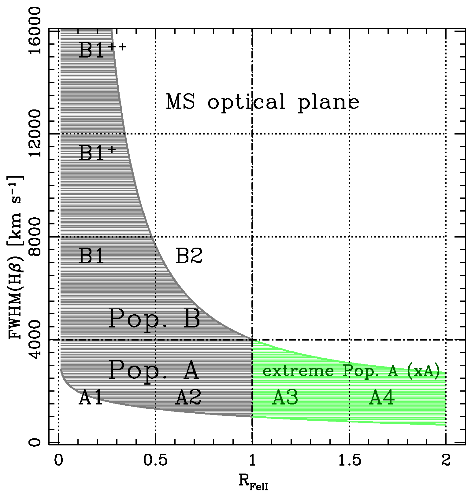
Nonetheless, new developments in the past decades have paved the road to the possibility of exploiting quasars as cosmological distance indicators in a novel way that would make them literal “Eddington standard candles” (ESC) ([17,18,19,20]; see also [21] for a comprehensive review of secondary distance indicators including several techniques based on quasars). This possibility is based in the development of the concept of a quasar main sequence (MS), intended to provide a sort of H-R diagram for quasars [22]. The quasar MS can be traced in the plane defined by the prominence of optical FeII emission, = I(FeII 4570)/I(H) (see [15,23,24,25,26]). Figure 1 provides a sketch of the MS in the optical plane FWHM(H) vs. . It is possible to isolate spectral types in the optical plane of the MS as a function of and FWHM H and, at a coarser level, two populations: Population A (FWHM H 4000 km/s) and Population B of broader sources. Pop. A is rather heterogeneous, and encompasses a range of from almost 0 to the highest values observed ( are very rare, ≲1% in optically-selected samples, [25]). Along the quasar main sequence, the extreme Population A (xA) sources satisfying the condition (about 10% of all quasars in optically-selected sample, green area in Figure 1) show remarkably low optical variability, so low that it is even difficult to estimate the BLR radius via reverberation mapping [27]. This is at variance with Pop. B sources that show more pronounced variability [28,29], the most extreme cases being observed among blazars which are low-accretors, at the opposite end in the quasar MS. Of the many multi-frequency trends along the main sequence (from the sources whose spectra show the broadest LILs (extreme Pop. B), and the weakest FeII emission, to sources with the narrowest LIL profiles and strongest FeII emission [extreme Pop. A]), we recall a systematic decrease of the CIV equivalent width, an increase in metallicity, and amplitude of HIL blueshifts (a more exhaustive list is provided by Table 1 of [30]). The Eddington ratio is believed to increase along with [23,26,31,32]. The FWHM H is strongly affected by the viewing angle (i.e., the angle between the line of sight and the accretion disk axis), so that at least the most narrow-line Seyfert 1s (NLSy1s) can be interpreted as Pop. A sources seen with the accretion disk oriented face-on or almost so [33]. At low-z (≲0.7), Pop. A implies low black hole mass , and high Eddington ratio; on the converse, Pop. B is associated with high and low . This trend follows from the “downsizing” of nuclear activity at low-z that helps give an elbow shape to the MS [34]: at low-z, very massive quasars ( M) do not radiate close to their Eddington limit but are, conversely, low-radiators ().
The inter-comparison between CIV1549 and H supports low-ionization lines virial broadening (in a system of dense clouds or in the accretion disk) + high-ionization lines (HILs) radial or vertical outflows, at least in Pop. A sources [35,36]. There is now a wide consensus on an accretion disk + wind system model [37], and therefore on the existence of a “virialized” low-ionization subregion + higher ionization, with the subregion outflowing up to the highest quasar luminosities [36,38,39].
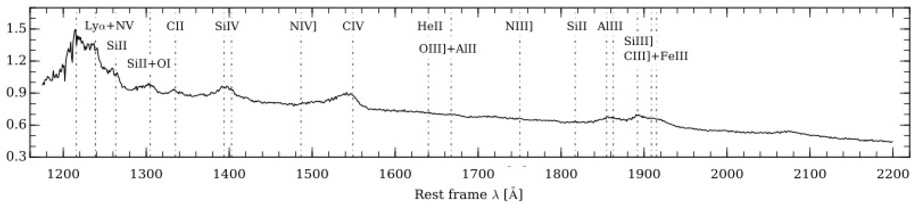
The most extreme examples at high accretion rate are a population of sources with distinguishing properties. They have been called extreme Pop. A or extreme quasars (xA), and are also known as super-Eddington accreting massive black holes (SEAMBHs) [9,18,40,41]. Figure 2 shows a composite rest-frame UV spectrum of high-luminosity xA quasars. Observationally, xA quasars satisfy and still show LIL H profiles basically consistent with emission from a virialized system. xA quasars may well represent an early stage in the evolution of quasars and galaxies. In the hierarchical growth scenario for the evolution of galaxies, merging and strong interaction lead to accumulation of gas in the galaxy central regions, inducing enhanced star formation. Strong winds from massive stars and eventual Supernova explosions may ultimately provide enriched accretion fuel for the massive black hole at the galaxy [42,43,44]. The active nucleus radiation force and the mechanical thrust of the accretion disk wind can then sweep the dust surrounding the black hole, at least within a cone coaxial with the accretion disk axis (see Figure 7 of [45]). The fraction of mass that is accreted by the black hole and the fraction that is instead ejected in the wind are highly uncertain; the outflow kinetic power can become comparable to the radiative output [46,47], especially in sources accreting at very high rate [48]; interestingly, this seems to be true also for stellar-mass black holes [49]. Feedback effects on the host galaxies are maximized by the high kinetic power of the wind, presumably made of gas much enriched in metals [50].
3. Diagnostics of Mildly-Ionized Gases
Diagnostics from the rest-frame UV spectrum takes advantage of the observations of strong resonance lines that are collisionally excited [51,52]. The point is that the rest-frame UV spectrum offers rich diagnostics that constrains at least gas density , ionization parameter U, and chemical abundance Z. For instance, Si II 1814/Si III] 1892 is sensitive to ionization CIV1549/Ly, CIV1549/(Si IV + OIV])1400, CIV1549/HeII1640, NV1240/HeII1640 are sensitive to metallicity; and Al III1860/Si III]1892, Si III]1892/CIII]1909 are sensitive to density, since inter-combination lines have a well defined critical density [51].
The photoionization code Cloudy models the ionization, chemical, and thermal state of gas exposed to a radiation field, and predicts its emission spectra and physical parameters [53,54]. In Cloudy, collisional excitation and radiative processes typical of mildly ionized gases are included. Cloudy simulation requires inputs in terms of , U, Z, quasar spectral energy distribution (SED), and column density . The ionization parameter
where is the number of ionizing photons, provides the ratio between photon and hydrogen number density. More importantly, the inversion of equation provides a measure of the emitting region radius once the ionizing photon flux i.e., the product is known. As we will see, the photon flux can be estimated with good precision from diagnostic line intensity ratios.
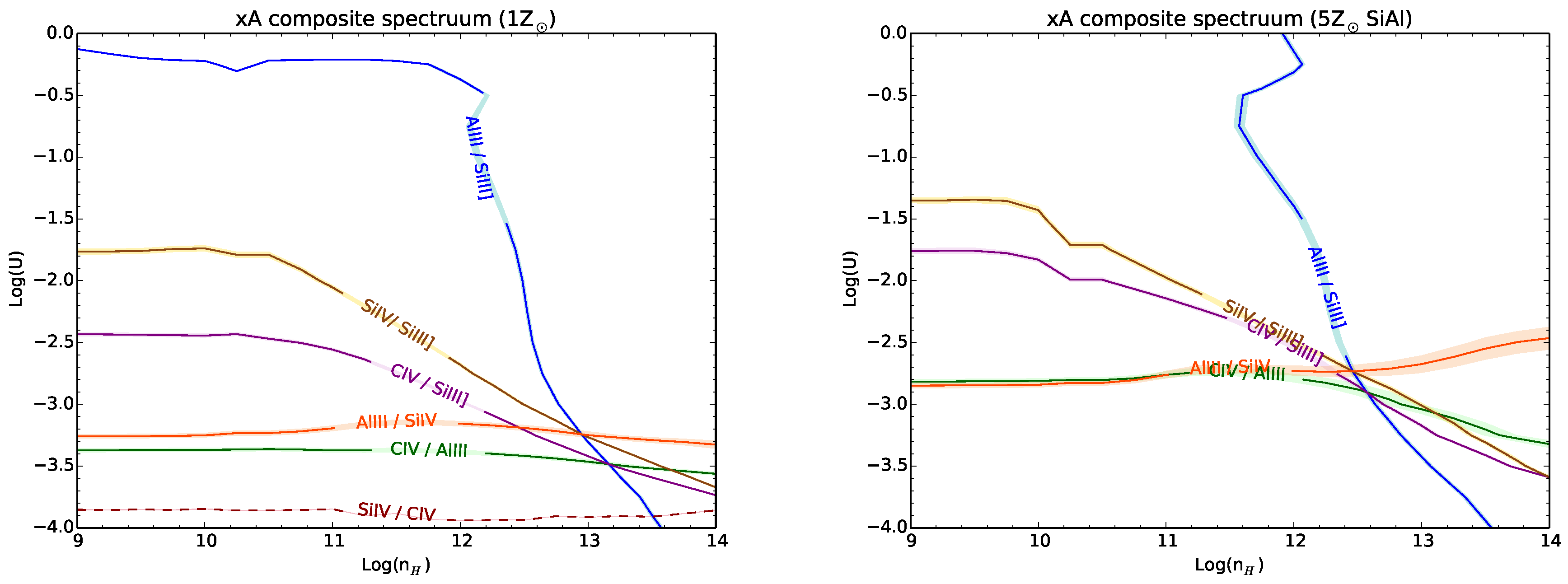
Maps built on an array of 551 Cloudy 08.00–13.00 photoionization models for a given metallicity Z and , constant n and U evaluated at steps of 0.25 dex covering the ranges [cm], . Given the measured intensity ratios for xA quasars, Cloudy simulations show convergence toward a well-defined value of log () [40,51]. UV diagnostic ratios in the plane ionization parameter versus density indicate extremely high cm, extremely low (Figure 3). Note the orthogonal information provided by the AlIII1860/SiIII]1892 that mainly depends on density. The left and right panels differ because of chemical abundances: the case with five times solar metallicity plus overabundance of Si and Al produces better agreement, displacing the solution toward lower density and higher ionization. Nonetheless, the product remains fairly constant. Diagnostic ratios sensible to chemical composition suggest high metallicity. The metallicities in the quasar BLR gas are a function of the spectral type (ST) along the MS: relatively low (solar or slightly sub-solar in extreme Pop. B sources (as estimated recently for NGC 1275 [55]), and relatively high for typical Pop. A quasars with moderate FeII emission (, [56,57]). If the diagnostic ratios are interpreted in terms of scaled , they may reach , even for xA quasars [40]. Z values as high as are likely to be unphysical, and suggest relative abundances of elements deviating from solar values, as assumed in the previous example, or significant turbulence. The analysis of the gas chemical composition in the BLR of xA source has just begun. However, high or non-solar Z are in line with the idea of xA sources being high accretors surrounded by huge amount of gas and a circum-nuclear star forming system, possibly with a top-heavy initial mass function [51]. The high is consistent with the low CIII]1909 emission that becomes undetectable in some cases. While in Pop. A and B we find evidence of ionization stratification within the low-ionization part of the BLR ([58,59,60] and references therein), xA sources show intensity ratios that are consistent with a very dense “remnant” of the BLR, perhaps after lower density gas has been ablated away by radiation forces.
4. xA Quasars as Eddington Standard Candles
There are several key elements that make it possible to exploit xA quasars as Eddington standard candles.
The first is the similarity of their spectra and hence of the physical condition in the mildly-ionized gas that is emitting the LILs. Line intensity ratios are similar (they scatter around a constant average with small dispersion). Since the line emitting gas is photoionized, intensity line ratios depend strongly on the ionizing continuum SED. Thus, the ionizing SED is also constrained within a small scatter. We remark that this is not true for the general population of quasars that show differences in line equivalent width and intensity ratios larger than an order of magnitude along the MS.
The mass reservoir in all xA sources is sufficient to ensure a very high accretion rate (possibly super-Eddington) that yields a radiative output close to the Eddington limit. The similarity of the SED and the presence of high rates of circumnuclear and galactic star formation as revealed by Spitzer [61] have led to the conjecture that xA sources may be in a particular stage of a quasar development, as mentioned above.
The second key element is the existence of a virialized low-ionization sub-region (possibly the accretion disk itself). This region coexists with outflowing gas even at extreme erg s and highest Eddington ratios but is kinematically distinguishable on the basis of inter-line shifts between LILs and HILs—for example, H and CIV1549.
In addition, xA quasars show extreme along the MS with small dispersion. If the Eddington ratio is known, and constant, then . Accretion disk theory teaches low radiative efficiency at a high accretion rate, and that ל saturates toward a limiting value ([62,63,64] and references therein). Therefore, empirical evidence (the xA class of sources, easily identified by their self-similar properties, scatters around a well-defined, extremal ל) and theoretical support (the saturation of the radiative output per unit ) justified the consideration of xA sources potential ESCs.
Virial Luminosity
The use of xA sources as Eddington standard candles requires several steps which should considered carefully.
- The first step is the actual estimate of the accretion luminosity via a virial broadening estimator (VBE). The luminosity can be written asassuming virial motions of the low-ionionization part of the broad-line region (BLR). The stands for a suitable VBE, usually the width of a convenient LIL (in practice, the FWHM of H or even Pa, [65]).
- The can be estimated from the inversion of Equation (1) [51,52], again taking advantage of the fact that the ionizing photon flux shows a small scatter around a well defined value. In addition, another key assumption is thatEquation (3) implies that scales with the square root of the luminosity. This is needed to preserve the U parameter. If U were going to change, then the spectrum would also change as a function of luminosity. This is not evident comparing spectra over a wide luminosity range (4.5 dex), although some second order effects are possible.1
- We can therefore write the virial luminosity asMaking explicit the dependence of the number of ionizing photons on the SED, the virial luminosity becomes:where is the fraction of ionizing luminosity scaled to 0.5, the average frequency of ionizing photons scaled to Hz, and to .
5. Selection of Eddington Standard Candles
Selection criteria are based on emission line intensity ratios which are extreme along the quasar MS [20]:
- ,
- UV AlIII1860/SiIII]1892 ,
- SiIII]1892/CIII]1909 .
The first criterion can be easily applied to optical spectra of a large survey such as the SDSS for sources at . The second and third criterion can be applied to sources at for which the 1900 blend lines are shifted into the optical and near IR domains. UV and optical selection criterions are believed to be equivalent. Due to a small sample size at low z for which rest-frame optical and UV spectra are available, further testing is needed.
6. Tentative Applications to Cosmology and the Future Perspectives
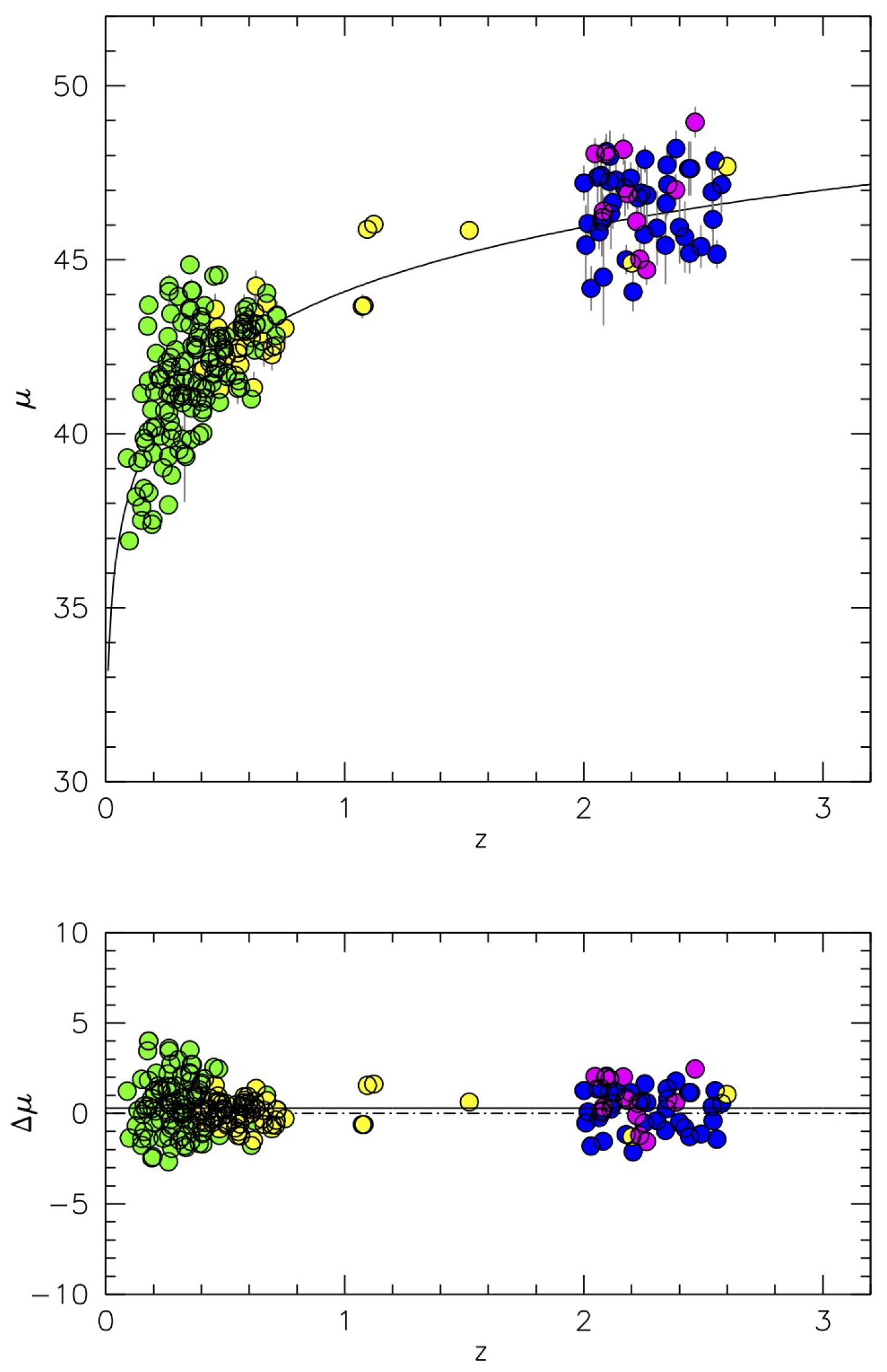
Preliminary results were collected from three quasar samples (62 sources in total), unevenly covering the redshift range . For redshift the UV AlIII1860 FWHM was used as a VBE for the rest-frame UV range, save a few cases for which H was available. This explorative application to cosmology yielded results consistent with concordance cosmology, and allowed the exclusion of some extreme cosmologies [20]. A more recent application involved the [20] sample, along with the H sample of [9] and preliminary measurements from [40]. The resulting Hubble diagram is shown in Figure 4. The plots in Figure 4 involve sources and indicate a scatter 1.2 mag. The slope of the residuals () is not significantly different from 0, indicating good statistical agreement between luminosities derived from concordance cosmological parameters and from the virial equation. The Hubble diagram of Figure 4 confirms the conceptual validity of the virial luminosity relation, Equation (5).
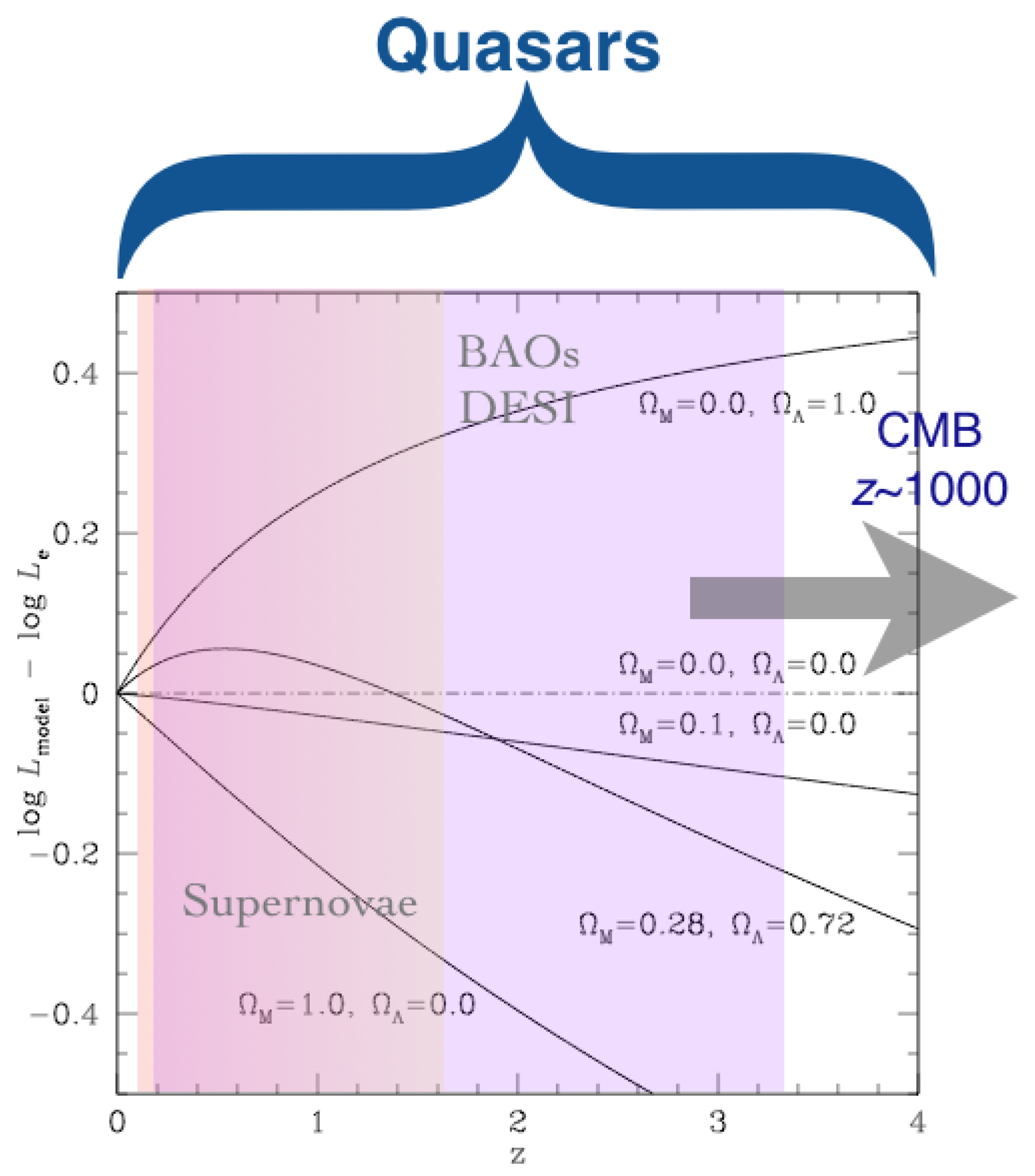
Mock samples of several hundreds of objects, even with significant dispersion in luminosity with rms() = 0.2–0.3, indicate that quasars covering the redshift range between 0 and 3 (i.e., a range of cosmic epochs from now to 2 Gyr since the Big Bang) could yield significant constraints on the cosmological parameters. A synthetic sample of 200 sources uniformly distributed in the redshift range 0–3 with a scatter of 0.2 dex yields at 1 confidence level, assuming km s Mpc, and flatness ( = 1). If is unconstrained, at 1 confidence level [20]. The comparison between the constraints set by supernova surveys and by a mock sample of 400 quasars with rms = 0.3 dex in shows the potential ability of the quasar sample to better constrain [70]. The scheme of Figure 5 illustrates the difference in sensitivity to cosmological parameters over the redshift range 0–4: supernovæ are sensitive to since the effect of , in a concordance cosmology scenario, became appreciable only at relatively recent cosmic epochs. High redshift quasars provide information on a redshift range where the expansion of the Universe was still being decelerated by the effect of , a range that is not yet covered by any standard ruler or candle.
Error Budget
The large scatter in the luminosity estimates is apparently daunting in the epoch of precision cosmology. Statistical errors could be reduced to rms dex in L by increasing numbers, collecting large samples (∼500 quasars), but they still would remain high.
The xA quasar SED cannot vary much since spectra are almost identical in terms of line ratios (a second order effect [72] not yet detected as significant in the data considered by [20,40] may become significant with larger samples). The scaling should hold strictly: a small deviation would imply a systematic change in the ionization parameter and hence of ST with luminosity.
A simplified error budget for statistical errors [20] indicates that virial luminosity estimates are mostly affected by VBE uncertainties which enter with the fourth power in Equation (5). In addition to measurement uncertainties, orientation effects are expected to be determinant in the FWHM uncertainties, as they can contribute 0.3 dex of scatter in luminosity if H or any other line used as a VBE is emitted in a highly-flattened configuration.2 Modeling the effect of orientation by computing the difference between L from concordance cosmology and virial luminosity indeed reduces the sample standard deviation in the Hubble diagram by a factor ≈5 to ≈0.2 mag, and accounts for most of the rms ≈ 0.4 dex in the virial luminosity estimates of the sample shown in Figure 4 [9]. The rms ≈ 0.2 mag value is comparable to the uncertainty in supernova magnitude measurements. Work is in progress in order to make viewing angle estimates of xA quasars usable for cosmology.
7. Conclusions
This paper provided an overview of the physical conditions in the broad line emitting region of extreme spectral types of type-1 quasars (the extreme Pop. A). There is strong evidence that xA sources are radiating close to their Eddington limit (i.e., with Eddington ratio scattering around a well-defined value), at high accretion rates. Their physical properties appear to be very stable across a very wide range of luminosity, 4–5 dex. The assumption of a constant ל makes it possible to write a relation between luminosity and virial broadening, analogous to the one expressed by the Tully–Fisher and the early formulation of Faber–Jackson laws.
The scatter in the Hubble diagram obtained from virial luminosity estimates is still very high, about 1 mag (although comparable to the scatter from a method based on the nonlinear relation between the X-ray and the UV emission of quasars [75]). Very large samples are needed for reduction of scatter (and statistical error). In addition, the inter-calibration of rest-frame visual and UV properties and their dependence on L (expect systematic errors!) needs to be extended by dedicated observations of xA sources covering the rest frame UV and visual range. Simulations of statistical and systematic effects which influence the estimates of the cosmic parameters are also needed.
In principle, Eddington standard candles can cover a range of distances where the metric of the Universe has not been “charted” as yet to retrieve an independent estimate of . If samples with uniform coverage over a wide range of redshift would become available, xA sources could also address the physics of accelerated expansion (i.e., provide measurements of the dark energy equation of state).
Author Contributions
E.B., N.B., A.d.O. and D.D. contributed with funding acquisition and resources. P.M., E.B., N.B., A.d.O., M.L.M.-A., C.A.N., M.D., G.M.S. significantly contributed to the papers on which this review is based. P.M. wrote the review paper.
Funding
P.M. wishes to thank the Scientific Organizing Committee of the Symposium on the Physics of Ionized Gases (SPIG 2018) meeting for inviting the topical lecture on which this paper is based, and acknowledges the Programa de Estancias de Investigación (PREI) No. DGAP/DFA/2192/2018 of Universidad Nacional Autónoma de México (UNAM), where this paper was written. The relevant research is part of the project 176001 “Astrophysical spectroscopy of extragalactic objects” and 176003 “Gravitation and the large scale structure of the Universe” supported by the Ministry of Education, Science and Technological Development of the Republic of Serbia. M.L.M.-A. acknowledges a CONACyT postdoctoral fellowship. A.d.O. and M.L.M.-A. acknowledge financial support from the Spanish Ministry for Economy and Competitiveness through Grant Nos. AYA2013-42227-P and AYA2016-76682-C3-1-P. M.L.M.-A, P.M. and M.D. acknowledge funding from the INAF PRIN-SKA 2017 program 1.05.01.88.04. D.D. and A.N. acknowledge support from CONACyT through Grant No. CB221398. D.D. and C.A.N. are also thankful for the support from Grant No. IN108716 53 PAPIIT, UNAM.
Conflicts of Interest
The authors declare no conflict of interest.
Abbreviations
The following abbreviations are used in this manuscript:
| AGN | Active Galactic Nucleus |
| BLR | Broad Line Region |
| DESI | Dark Energy Spectroscopic Instrument |
| ESC | Eddington Standard Candles |
| FWHM | Full Width Half-Maximum |
| HIL | High-Ionization Line |
| LIL | Low-Ionization Line |
| MDPI | Multidisciplinary Digital Publishing Institute |
| MS | Main Sequence |
| NLSy1 | Narrow-Line Seyfert 1 |
| SDSS | Sloan Digital Sly Survey |
| VBE | Virial Broadening Estimator |
References
- Vanden Berk, D.E.; Richards, G.T.; Bauer, A.; Strauss, M.A.; Schneider, D.P.; Heckman, T.M.; York, D.G.; Hall, P.B.; Fan, X.; Knapp, G.R.; et al. Composite Quasar Spectra from the Sloan Digital Sky Survey. Astron. J. 2001, 122, 549–564. [Google Scholar] [CrossRef]
- Marziani, P.; Dultzin-Hacyan, D.; Sulentic, J.W. Accretion onto Supermassive Black Holes in Quasars: Learning from Optical/UV Observations. In New Developments in Black Hole Research; Kreitler, P.V., Ed.; Nova Press: New York, NY, USA, 2006; p. 123. [Google Scholar]
- Netzer, H. AGN emission lines. In Active Galactic Nuclei; Blandford, R.D., Netzer, H., Woltjer, L., Courvoisier, T.J.-L., Mayor, M., Eds.; Springer: Berlin/Heidelberg, Germany, 1990; pp. 57–160. [Google Scholar]
- Marinello, A.O.M.; Rodriguez-Ardila, A.; Garcia-Rissmann, A.; Sigut, T.A.A.; Pradhan, A.K. The FeII emission in active galactic nuclei: Excitation mechanisms and location of the emitting region. arXiv, 2016; arXiv:1602.05159. [Google Scholar]
- Antonucci, R. Unified models for active galactic nuclei and quasars. Annu. R. Astron. Astrophys. 1993, 31, 473–521. [Google Scholar] [CrossRef]
- D’Onofrio, M.; Burigana, C. Questions of Modern Cosmology: Galileo’s Legacy; Springer: Berlin/Heidelberg, Germany, 2009. [Google Scholar] [CrossRef]
- Pâris, I.; Petitjean, P.; Aubourg, É.; Myers, A.D.; Streblyanska, A.; Lyke, B.W.; Anderson, S.F.; Armengaud, É.; Bautista, J.; Blanton, M.R.; et al. The Sloan Digital Sky Survey Quasar Catalog: Fourteenth data release. Astron. Astrophys. 2018, 613, A51. [Google Scholar] [CrossRef]
- Marziani, P.; Dultzin, D.; Sulentic, J.W.; Del Olmo, A.; Negrete, C.A.; Martinez-Aldama, M.L.; D’Onofrio, M.; Bon, E.; Bon, N.; Stirpe, G.M. A main sequence for quasars. Front. Astron. Space Sci. 2018, 5, 6. [Google Scholar] [CrossRef]
- Negrete, C.A.; Dultzin, D.; Marziani, P.; Esparza, D.; Sulentic, J.W.; del Olmo, A.; Martínez-Aldama, M.L.; García López, A.; D’Onofrio, M.; Bon, N.; et al. Highly accreting quasars: The SDSS low-redshift catalog. Astron. Astrophys. 2018, 620, A118. [Google Scholar] [CrossRef]
- Liu, Y.; Jiang, D.R.; Gu, M.F. The Jet Power, Radio Loudness, and Black Hole Mass in Radio-loud Active Galactic Nuclei. Astrophys. J. 2006, 637, 669–681. [Google Scholar] [CrossRef]
- Bon, E.; Zucker, S.; Netzer, H.; Marziani, P.; Bon, N.; Jovanović, P.; Shapovalova, A.I.; Komossa, S.; Gaskell, C.M.; Popović, L.Č.; et al. Evidence for Periodicity in 43 year-long Monitoring of NGC 5548. Astrophys. J. Suppl. Ser. 2016, 225, 29. [Google Scholar] [CrossRef]
- Bon, E.; Marziani, P.; Bon, N. Periodic optical variability of AGN. IAU Symp. 2017, 324, 176–179. [Google Scholar] [CrossRef]
- Netzer, H. Meeting Summary: A 2017 View of Active Galactic Nuclei. Front. Astron. Space Sci. 2018, 5, 10. [Google Scholar] [CrossRef]
- Marziani, P.; D’Onofrio, M.; del Olmo, A.; Dultzin, D. (Eds.) Quasars at All Cosmic Epochs; Frontiers Media: Lausanne, Switzerland, 2018. [Google Scholar] [CrossRef]
- Sulentic, J.W.; Marziani, P.; Dultzin-Hacyan, D. Phenomenology of Broad Emission Lines in Active Galactic Nuclei. Annu. Rev. Astron. Astrophys. 2000, 38, 521–571. [Google Scholar] [CrossRef]
- Baldwin, J.A.; Burke, W.L.; Gaskell, C.M.; Wampler, E.J. Relative quasar luminosities determined from emission line strengths. Nature 1978, 273, 431–435. [Google Scholar] [CrossRef]
- Teerikorpi, P. On Öpik’s distance evaluation method in a cosmological context. Astron. Astrophys. 2011, 531, A10. [Google Scholar] [CrossRef]
- Wang, J.M.; Du, P.; Valls-Gabaud, D.; Hu, C.; Netzer, H. Super-Eddington Accreting Massive Black Holes as Long-Lived Cosmological Standards. Phys. Rev. Lett. 2013, 110, 081301. [Google Scholar] [CrossRef] [PubMed]
- Wang, J.M.; Du, P.; Li, Y.R.; Ho, L.C.; Hu, C.; Bai, J.M. A New Approach to Constrain Black Hole Spins in Active Galaxies Using Optical Reverberation Mapping. Astrophys. J. Lett. 2014, 792, L13. [Google Scholar] [CrossRef]
- Marziani, P.; Sulentic, J.W. Highly accreting quasars: Sample definition and possible cosmological implications. Mon. Not. R. Astron. Soc. 2014, 442, 1211–1229. [Google Scholar] [CrossRef]
- Czerny, B.; Beaton, R.; Bejger, M.; Cackett, E.; Dall’Ora, M.; Holanda, R.F.L.; Jensen, J.B.; Jha, S.W.; Lusso, E.; Minezaki, T.; et al. Astronomical Distance Determination in the Space Age. Secondary Distance Indicators. Space Sci. Rev. 2018, 214, 32. [Google Scholar] [CrossRef]
- Sulentic, J.W.; Zamfir, S.; Marziani, P.; Dultzin, D. Our Search for an H-R Diagram of Quasars. Revista Mexicana de Astronomia y Astrofisica Conference Series 2008, 32, 51–58. [Google Scholar]
- Boroson, T.A.; Green, R.F. The emission-line properties of low-redshift quasi-stellar objects. Astrophys. J. Suppl. Ser. 1992, 80, 109–135. [Google Scholar] [CrossRef]
- Sulentic, J.W.; Marziani, P.; Zamanov, R.; Bachev, R.; Calvani, M.; Dultzin-Hacyan, D. Average Quasar Spectra in the Context of Eigenvector 1. Astrophys. J. Lett. 2002, 566, L71–L75. [Google Scholar] [CrossRef]
- Zamfir, S.; Sulentic, J.W.; Marziani, P.; Dultzin, D. Detailed characterization of Hβ emission line profile in low-z SDSS quasars. Mon. Not. R. Astron. Soc. 2010, 403, 1759. [Google Scholar] [CrossRef]
- Shen, Y.; Ho, L.C. The diversity of quasars unified by accretion and orientation. Nature 2014, 513, 210–213. [Google Scholar] [CrossRef] [PubMed]
- Du, P.; Zhang, Z.X.; Wang, K.; Huang, Y.K.; Zhang, Y.; Lu, K.X.; Hu, C.; Li, Y.R.; Bai, J.M.; Bian, W.H.; et al. Supermassive Black Holes with High Accretion Rates in Active Galactic Nuclei. IX. 10 New Observations of Reverberation Mapping and Shortened Hβ Lags. Astrophys. J. 2018, 856, 6. [Google Scholar] [CrossRef]
- Dultzin-Hacyan, D.; Schuster, W.J.; Parrao, L.; Pena, J.H.; Peniche, R.; Benitez, E.; Costero, R. Optical variability of the Seyfert nucleus NGC 7469 in timescales from days to minutes. Astron. J. 1992, 103, 1769–1787. [Google Scholar] [CrossRef]
- Giveon, U.; Maoz, D.; Kaspi, S.; Netzer, H.; Smith, P.S. Long-term optical variability properties of the Palomar-Green quasars. Mon. Not. R. Astron. Soc. 1999, 306, 637–654. [Google Scholar] [CrossRef]
- Sulentic, J.; Marziani, P.; Zamfir, S. The Case for Two Quasar Populations. Balt. Astron. 2011, 20, 427–434. [Google Scholar] [CrossRef]
- Kuraszkiewicz, J.K.; Green, P.J.; Crenshaw, D.M.; Dunn, J.; Forster, K.; Vestergaard, M.; Aldcroft, T.L. Emission Line Properties of Active Galactic Nuclei from a Post-COSTAR Hubble Space Telescope Faint Object Spectrograph Spectral Atlas. Astrophys. J. Suppl. Ser. 2004, 150, 165–180. [Google Scholar] [CrossRef]
- Sun, J.; Shen, Y. Dissecting the Quasar Main Sequence: Insight from Host Galaxy Properties. Astrophys. J. Lett. 2015, 804, L15. [Google Scholar] [CrossRef]
- Dultzin, D.; Martinez, M.L.; Marziani, P.; Sulentic, J.W.; Negrete, A. Narrow-Line Seyfert 1s: A luminosity dependent definition. In Proceedings of the Conference “Narrow-Line Seyfert 1 Galaxies and Their Place in the Universe”, Milano, Italy, 4–6 April 2011. [Google Scholar]
- Fraix-Burnet, D.; Marziani, P.; D’Onofrio, M.; Dultzin, D. The Phylogeny of Quasars and the Ontogeny of Their Central Black Holes. Front. Astron. Space Sci. 2017, 4, 1. [Google Scholar] [CrossRef]
- Leighly, K.M. Hubble Space Telescope STIS Ultraviolet Spectral Evidence of Outflow in Extreme Narrow-Line Seyfert 1 Galaxies. II. Modeling and Interpretation. Astrophys. J. 2004, 611, 125–152. [Google Scholar] [CrossRef]
- Sulentic, J.W.; del Olmo, A.; Marziani, P.; Martínez-Carballo, M.A.; D’Onofrio, M.; Dultzin, D.; Perea, J.; Martínez-Aldama, M.L.; Negrete, C.A.; Stirpe, G.M.; et al. What does Civλ1549 tell us about the physical driver of the Eigenvector Quasar Sequence? arXiv, 2017; arXiv:1708.03187. [Google Scholar]
- Elvis, M. A Structure for Quasars. Astrophys. J. 2000, 545, 63–76. [Google Scholar] [CrossRef]
- Bisogni, S.; di Serego Alighieri, S.; Goldoni, P.; Ho, L.C.; Marconi, A.; Ponti, G.; Risaliti, G. Simultaneous detection and analysis of optical and ultraviolet broad emission lines in quasars at z 2.2. arXiv, 2017; arXiv:1702.08046. [Google Scholar]
- Vietri, G.; Piconcelli, E.; Bischetti, M.; Duras, F.; Martocchia, S.; Bongiorno, A.; Marconi, A.; Zappacosta, L.; Bisogni, S.; Bruni, G.; et al. The WISSH Quasars Project IV. BLR versus kpc-scale winds. arXiv, 2018; arXiv:1802.03423. [Google Scholar]
- Martínez-Aldama, M.L.; Del Olmo, A.; Marziani, P.; Sulentic, J.W.; Negrete, C.A.; Dultzin, D.; D’Onofrio, M.; Perea, J. Extreme quasars at high redshift. Astron. Astroph. 2018, 618, A179. [Google Scholar] [CrossRef]
- Du, P.; Lu, K.X.; Hu, C.; Qiu, J.; Li, Y.R.; Huang, Y.K.; Wang, F.; Bai, J.M.; Bian, W.H.; Yuan, Y.F.; et al. Supermassive Black Holes with High Accretion Rates in Active Galactic Nuclei. VI. Velocity-resolved Reverberation Mapping of the Hβ Line. Astrophys. J. 2016, 820, 27. [Google Scholar] [CrossRef]
- Heller, C.H.; Shlosman, I. Fueling nuclear activity in disk galaxies: Starbursts and monsters. Astrophys. J. 1994, 424, 84–105. [Google Scholar] [CrossRef]
- Collin, S.; Zahn, J.P. Star formation and evolution in accretion disks around massive black holes. Annu. Rev. Astron. Astrophys. 1999, 344, 433–449. [Google Scholar]
- Williams, R.J.R.; Baker, A.C.; Perry, J.J. Symbiotic starburst-black hole active galactic nuclei—I. Isothermal hydrodynamics of the mass-loaded interstellar medium. Mon. Not. R. Astron. Soc. 1999, 310, 913–962. [Google Scholar] [CrossRef]
- D’Onofrio, M.; Marziani, P. A Multimessenger View of Galaxies and Quasars From Now to Mid-century. Front. Astron. Space Sci. 2018, 5, 31. [Google Scholar] [CrossRef]
- King, A.; Pounds, K. Powerful Outflows and Feedback from Active Galactic Nuclei. Annu. R. Astron. Astrophys. 2015, 53, 115–154. [Google Scholar] [CrossRef]
- Marziani, P.; Negrete, C.A.; Dultzin, D.; Martínez-Aldama, M.L.; Del Olmo, A.; D’Onofrio, M.; Stirpe, G.M. Quasar massive ionized outflows traced by CIV λ1549 and [OIII]λλ4959,5007. Front. Astron. Space Sci. 2017, 4, 16. [Google Scholar] [CrossRef]
- Nardini, E.; Reeves, J.N.; Gofford, J.; Harrison, F.A.; Risaliti, G.; Braito, V.; Costa, M.T.; Matzeu, G.A.; Walton, D.J.; Behar, E.; et al. Black hole feedback in the luminous quasar PDS 456. Science 2015, 347, 860–863. [Google Scholar] [CrossRef] [PubMed]
- Tetarenko, B.E.; Lasota, J.P.; Heinke, C.O.; Dubus, G.; Sivakoff, G.R. Strong disk winds traced throughout outbursts in black-hole X-ray binaries. Nature 2018, 554, 69. [Google Scholar] [CrossRef] [PubMed]
- Baskin, A.; Laor, A. Metal enrichment by radiation pressure in active galactic nucleus outflows - theory and observations. Mon. Not. R. Astron. Soc. 2012, 426, 1144–1158. [Google Scholar] [CrossRef]
- Negrete, A.; Dultzin, D.; Marziani, P.; Sulentic, J. BLR Physical Conditions in Extreme Population A Quasars: A Method to Estimate Central Black Hole Mass at High Redshift. Astrophys. J. 2012, 757, 62. [Google Scholar] [CrossRef]
- Negrete, C.A.; Dultzin, D.; Marziani, P.; Sulentic, J.W. Reverberation and Photoionization Estimates of the Broad-line Region Radius in Low-z Quasars. Astrophys. J. 2013, 771, 31. [Google Scholar] [CrossRef]
- Ferland, G.J.; Porter, R.L.; van Hoof, P.A.M.; Williams, R.J.R.; Abel, N.P.; Lykins, M.L.; Shaw, G.; Henney, W.J.; Stancil, P.C. The 2013 Release of Cloudy. Revista Mexicana de Astronomía y Astrofísica 2013, 49, 137–163. [Google Scholar]
- Ferland, G.J.; Chatzikos, M.; Guzmán, F.; Lykins, M.L.; van Hoof, P.A.M.; Williams, R.J.R.; Abel, N.P.; Badnell, N.R.; Keenan, F.P.; Porter, R.L.; et al. The 2017 Release Cloudy. Revista Mexicana de Astronomía y Astrofísica 2017, 53, 385–438. [Google Scholar]
- Punsly, B.; Marziani, P.; Bennert, V.N.; Nagai, H.; Gurwell, M.A. Revealing the Broad Line Region of NGC 1275: The Relationship to Jet Power. Astrophys. J. 2018, 869, 143. [Google Scholar] [CrossRef]
- Shin, J.; Woo, J.H.; Nagao, T.; Kim, S.C. The Chemical Properties of Low-redshift QSOs. Astrophys. J. 2013, 763, 58. [Google Scholar] [CrossRef]
- Sulentic, J.W.; Marziani, P.; del Olmo, A.; Dultzin, D.; Perea, J.; Alenka Negrete, C. GTC spectra of z ≈ 2.3 quasars: Comparison with local luminosity analogs. Astron. Astrophys. 2014, 570, A96. [Google Scholar] [CrossRef]
- Peterson, B.M.; Wandel, A. Evidence for Supermassive Black Holes in Active Galactic Nuclei from Emission-Line Reverberation. Astrophys. J. Lett. 2000, 540, L13–L16. [Google Scholar] [CrossRef]
- Peterson, B.M.; Wandel, A. Keplerian Motion of Broad-Line Region Gas as Evidence for Supermassive Black Holes in Active Galactic Nuclei. Astrophys. J. Lett. 1999, 521, L95–L98. [Google Scholar] [CrossRef]
- Gaskell, C.M. What broad emission lines tell us about how active galactic nuclei work. New Astron. Rev. 2009, 53, 140–148. [Google Scholar] [CrossRef]
- Sani, E.; Lutz, D.; Risaliti, G.; Netzer, H.; Gallo, L.C.; Trakhtenbrot, B.; Sturm, E.; Boller, T. Enhanced star formation in narrow-line Seyfert 1 active galactic nuclei revealed by Spitzer. Mon. Not. R. Astron. Soc. 2010, 403, 1246–1260. [Google Scholar] [CrossRef]
- Abramowicz, M.A.; Czerny, B.; Lasota, J.P.; Szuszkiewicz, E. Slim accretion disks. Astrophys. J. 1988, 332, 646–658. [Google Scholar] [CrossRef]
- Mineshige, S.; Kawaguchi, T.; Takeuchi, M.; Hayashida, K. Slim-Disk Model for Soft X-Ray Excess and Variability of Narrow-Line Seyfert 1 Galaxies. Publ. Astron. Soc. Jpn. 2000, 52, 499–508. [Google Scholar] [CrossRef]
- Abramowicz, M.A.; Straub, O. Accretion discs. Scholarpedia 2014, 9, 2408. [Google Scholar] [CrossRef]
- La Franca, F.; Bianchi, S.; Ponti, G.; Branchini, E.; Matt, G. A New Cosmological Distance Measure Using Active Galactic Nucleus X-Ray Variability. Astrophys. J. Lett. 2014, 787, L12. [Google Scholar] [CrossRef]
- Tully, R.B.; Fisher, J.R. A new method of determining distances to galaxies. Astron. Astrophys. 1977, 54, 661–673. [Google Scholar]
- Faber, S.M.; Jackson, R.E. Velocity dispersions and mass-to-light ratios for elliptical galaxies. Astrophys. J. 1976, 204, 668–683. [Google Scholar] [CrossRef]
- Martínez-Aldama, M.L.; Del Olmo, A.; Marziani, P.; Sulentic, J.W.; Negrete, C.A.; Dultzin, D.; Perea, J.; D’Onofrio, M. Highly Accreting Quasars at High Redshift. Front. Astron. Space Sci. 2018, 4, 65. [Google Scholar] [CrossRef]
- Marziani, P.; Negrete, C.A.; Dultzin, D.; Martinez-Aldama, M.L.; Del Olmo, A.; Esparza, D.; Sulentic, J.W.; D’Onofrio, M.; Stirpe, G.M.; Bon, E.; et al. Highly accreting quasars: A tool for cosmology? IAU Symp. 2017, 324, 245–246. [Google Scholar] [CrossRef]
- Marziani, P.; Sulentic, J.W. Quasars and their emission lines as cosmological probes. Adv. Space Res. 2014, 54, 1331–1340. [Google Scholar] [CrossRef]
- Levi, M.; Bebek, C.; Beers, T.; Blum, R.; Cahn, R.; Eisenstein, D.; Flaugher, B.; Honscheid, K.; Kron, R.; Lahav, O.; et al. The DESI Experiment, a whitepaper for Snowmass 2013. arXiv, 2013; arXiv:1308.0847. [Google Scholar]
- Shemmer, O.; Lieber, S. Weak Emission-line Quasars in the Context of a Modified Baldwin Effect. Astrophys. J. 2015, 805, 124. [Google Scholar] [CrossRef]
- Jarvis, M.J.; McLure, R.J. Orientation dependency of broad-line widths in quasars and consequences for black hole mass estimation. Mon. Not. R. Astron. Soc. 2006, 369, 182–188. [Google Scholar] [CrossRef]
- Marziani, P.; Olmo, A.; Martínez-Aldama, M.; Dultzin, D.; Negrete, A.; Bon, E.; Bon, N.; D’Onofrio, M. Quasar Black Hole Mass Estimates from High-Ionization Lines: Breaking a Taboo? Atoms 2017, 5, 33. [Google Scholar] [CrossRef]
- Risaliti, G.; Lusso, E. A Hubble Diagram for Quasars. Astrophys. J. 2015, 815, 33. [Google Scholar] [CrossRef]
| 1 | The maximum temperature of the accretion disk is ; the SED is expected to become softer at high , but this effect has not been detected yet at a high confidence level. |
| 2 |
Figure 1.
The plane FWHM(H) vs. . The MS is sketched as the grey strip, with the section occupied by xA sources colored pale green. The thick dot-dashed line separates Pop. A and B at 4000 km s, while the vertical one at = 1 traces the lower value for xA identification. The spectral types with significant occupation at low-z are labeled.

Figure 2.
Composite UV spectrum of high-z xA sources. The abscissa is rest-frame wavelength, and the ordinate is normalized flux.
Figure 2.
Composite UV spectrum of high-z xA sources. The abscissa is rest-frame wavelength, and the ordinate is normalized flux.

Figure 3.
Intensity ratios in the plane ionization parameter vs. density, for the intensity ratios measured on the composite xA quasar spectrum shown in Figure 2 of [40]. left panel: solar chemical composition; right: solar chemical composition with selective enrichment in Al and Si, following [51]. In this latter case, the SiIV1402/CIV1549 is degenerate.

Figure 4.
Hubble diagram distance modulus vs. z obtained from the analysis of the [20] data (yellow: H, navy blue: Aliii1860 and Siiii]1892) supplemented by new H measurements from the SDSS obtained in this work (green) and from Gran Telescopio Canarias (GTC) observations of Martinez-Aldama et al. [68] (magenta). The lower panel shows the distance modulus residuals with respect to concordance cosmology. The filled line in the upper panel is the (z) expected from cold dark matter (CDM) cosmology. The filled line in the lower panel represents a least-square fit to the residuals as a function of z. The figure is an updated version of Figure 1 of Marziani et al. [69].

Figure 5.
Luminosity difference with respect to an empty Universe for several cosmological models, identified by their values of and . The domain of supernovæ and of the baryonic acoustic oscillations (within the expectation of the future Dark Energy Spectroscopic Instrument (DESI) survey, [71]) are shown.

© 2019 by the authors. Licensee MDPI, Basel, Switzerland. This article is an open access article distributed under the terms and conditions of the Creative Commons Attribution (CC BY) license (http://creativecommons.org/licenses/by/4.0/).
Share and Cite
MDPI and ACS Style
Marziani, P.; Bon, E.; Bon, N.; del Olmo, A.; Martínez-Aldama, M.L.; D’Onofrio, M.; Dultzin, D.; Negrete, C.A.; Stirpe, G.M. Quasars: From the Physics of Line Formation to Cosmology. Atoms 2019, 7, 18. https://doi.org/10.3390/atoms7010018
AMA Style
Marziani P, Bon E, Bon N, del Olmo A, Martínez-Aldama ML, D’Onofrio M, Dultzin D, Negrete CA, Stirpe GM. Quasars: From the Physics of Line Formation to Cosmology. Atoms. 2019; 7(1):18. https://doi.org/10.3390/atoms7010018
Chicago/Turabian StyleMarziani, Paola, Edi Bon, Natasa Bon, Ascension del Olmo, Mary Loli Martínez-Aldama, Mauro D’Onofrio, Deborah Dultzin, C. Alenka Negrete, and Giovanna M. Stirpe. 2019. "Quasars: From the Physics of Line Formation to Cosmology" Atoms 7, no. 1: 18. https://doi.org/10.3390/atoms7010018
Note that from the first issue of 2016, this journal uses article numbers instead of page numbers. See further details here.