1. Introduction
The Amazon-Andes transition in tropical South America represents an extensive hydro-climatic system coupled by the main large-scale circulation features and the barrier effect of the topography [
1,
2,
3]. Over the Amazon basin, large amounts of moisture are released into the atmosphere by evapotranspiration. The moisture-laden air masses are advanced to the Andes range by the easterly trade winds, where they fed by water resources such as forests, peatlands, and glaciers, through the formation of orographic induced precipitation [
4].
The atmospheric moisture transport in tropical South America is generally controlled by the seasonal cycle of the large-scale circulation features and the inter-hemispherical shift of the inter-tropical convergence zone (ITCZ). In the upper troposphere, during the austral summer months (December–February, DJF), the Bolivian high (BH) is well established and centered near 20° S and 60° W [
5]. In the lower troposphere, a deep low pressure system develops in the Chaco region (around 25° S, Chaco low) [
6], and the ITCZ is located in the Southern Hemisphere. Due to the height and length of the Andes, the terrain acts as a barrier, generating a climate divide between the western and eastern escarpment. While the eastern slopes are under the influence of the moisture-laden trade winds, the western slope experiences stable and, thus, drier conditions caused by the South Pacific high pressure system (SPH,
Figure 1a). During the austral winter months (June–August, JJA), the ITCZ migrates northward, and the central Andes have their main dry season. The SPH induces large-scale subsidence [
7], while in the upper atmosphere, a westerly flow blocks the transport of moisture from the Amazon. In contrast, the northern Andes experience rainy periods, due to the prevailing easterlies. Thus, the climate conditions exhibit both a strong zonal and meridional gradient. For more details on the South American monsoon system, see [
5,
8,
9,
10,
11,
12], among others.
As described by previous studies, this coupled hydro-climatic system between the Amazon basin and the Andes highlands is highly endangered by global change [
2,
13,
14,
15], which alters the evapotranspiration and moisture distribution. To understand the atmospheric moisture transport towards the Andean range on a regional scale, as well as the recycling of the water over the highlands, regional climate models (RCMs) provide a useful tool. RCMs are widely used to derive small-scale climate features using a dynamical downscaling approach [
16,
17]. The RCMs help to derive the necessary climate conditions for exploring and attributing recent and future trends. Moreover, in regions dominated by complex terrain as the Andes Mountains, RCMs provide an added value due to the better representation of the topographical characteristics driving the regional climate [
18,
19]. However, as is well known, dealing with RCMs requires specific considerations, since they are sensitive to the domain geometry and size [
20,
21], the driving fields [
22,
23], as well as the physical parametrizations [
24,
25]. Bowden et al. [
26] associated inconsistencies in RCMs with a misrepresentation of large-scale circulations. Due to the fact that large-scale atmospheric features determine the environment for small-scale processes [
8,
11], their accurate representation by an RCM is essential to reduce the model uncertainty. Wu et al. [
27] examined uncertainties in an RCM caused by the forcing fields. The authors highlighted that the bias from lateral boundary conditions (LBC) contributed more to the uncertainties in the RCM than the initial boundary conditions (IBC), because of the decreasing impact of IBC with increasing time. Although in a statistical downscaling study, Manzanas et al. [
28] also made evident that the choice of reanalysis data is an important contributor to uncertainties in the model results. A technique to reduce the uncertainties in the RCM is the spectral nudging towards the forcing fields. However, the technique has been successfully applied [
29,
30], but it is controversially discussed in the context of lacking the freedom of the large-scale circulation of the RCM [
31,
32]. Miguez-Macho et al. [
31] showed that using spectral nudging, small biases in the mid- and upper-tropospheric fields are generated, indicating that the large-scale circulation follows closely the observations. Liu et al. [
33] reported on the benefit of applying the spectral nudging technique in the WRF model over North America due to the capacity of balancing the performance at both large scales and small scales. With respect to typhoon tracking, Guo and Zhong [
34] demonstrated that using spectral nudging reduces the simulation error.
The ability of RCMs to capture the general climate features of South America and to enhance small-scale characteristics was presented by various studies, including [
35,
36,
37,
38], amongst other. However, most of the studies address rainfall patterns over Amazonian areas such as the South Atlantic convergence zone, the north-eastern region of Brazil, as well as the La Plata basin, and only few reported on rainfall behavior over the Andes Mountains, such as Da Rocha et al. [
38], Rojas [
39], Mourre et al. [
40], Junquas et al. [
41].
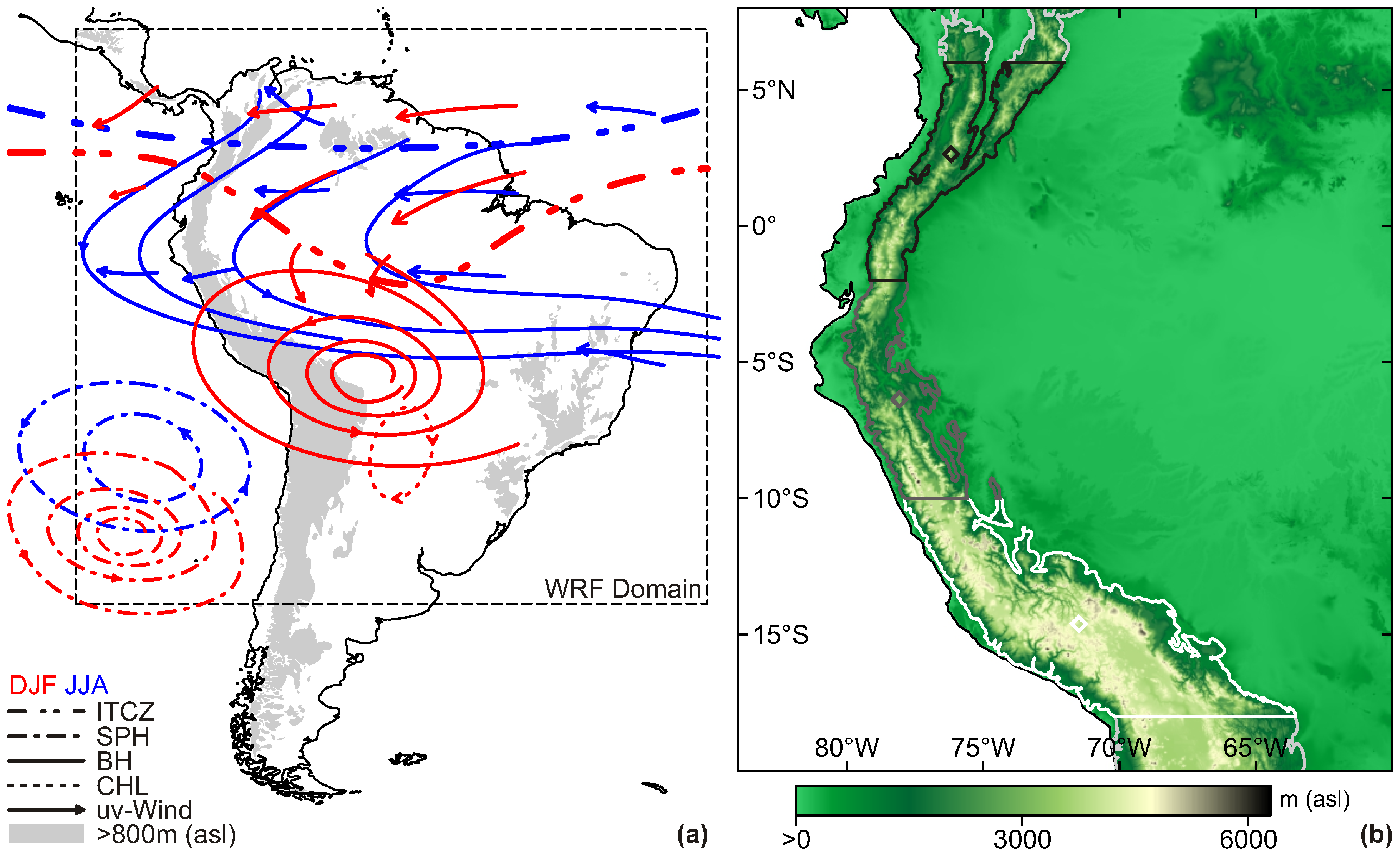
The objective of this study is the analysis of the atmospheric moisture pathways to the inter-Andean highlands as a precondition for the precipitation formation directly influencing the Andean water resources. For this, the Weather Research and Forecasting (WRF) model [
42], as well as back-trajectories applying the hybrid Lagrange integrated trajectory model (HYSPLIT) [
43] are used. Due to seasonal oscillations of the atmospheric environmental conditions inducing meridional differences along the Andes chain, three subregions in the highlands for the back-trajectory calculations are addressed (
Figure 1b). The regions are selected on the basis of a terrain contour above the 800-m asl height level (light gray filled contour in
Figure 1a) in the northern Andes (6° N– 2° S, N), the central tropical Andes (2° S–10° S, C), and the southern tropical Andes (10° S–18° S, S). The focus concerning the air mass pathways is on non-anomalous conditions related to the El Niño Southern Oscillation (ENSO) phenomenon.
Precipitation formation in the Andes Mountains is a complex interaction of large-scale environmental conditions providing the moisture and diurnal circulation patterns due to the complex structure of the terrain [
44,
45]. For the eastern slopes of the Ecuadorian Andes, Bendix et al. [
46] and Trachte et al. [
47] could demonstrate the formation of nocturnal convective clouds and the relation to rather weak large-scale conditions. At the western slopes of the Peruvian Andes, Trachte et al. [
48] presented varying air mass influences on the precipitation variability in the highlands and their dependence on the seasonal cycle. Insel et al. [
49] reported for the central Andes that the topography has a significant effect on the moisture transport between the Andes-Amazon transition through a topographical blocking of westerlies from the Pacific Ocean. However, despite the dominance of the easterlies in tropical South America, Makowski Giannoni et al. [
50] demonstrated for the northern Andes that air masses from the Pacific Ocean also reach the highlands of the eastern escarpment, although these transport pathways are less frequent. Thus, the main aim of this study is to investigate: (i) whether the Pacific atmospheric pathways contribute to the moisture transport to the Andean highlands; (ii) how the contribution of moisture differs along the meridional gradient; and (iii) how the seasonal oscillation of the large-scale drivers affects the atmospheric moisture pathways. To identify sources of model uncertainties according to both the regional atmospheric circulation and precipitation, we test two different dynamical downscaling methods (long-term integration and spectral nudging) using four different initial and lateral boundary conditions (ILBCs).
The paper is structured as follows: The next section describes the study area followed by the WRF and HYSPLIT model setup. The results are then examined and discussed in the context of the benefit of spectral nudging, as well as the driving fields representing the precipitation and the atmospheric moisture pathways to the three main study sites in the Andes.
2. Model Setup and Data
In these simulations, the Advanced Research WRF ([
42], Version 3.5) model was applied to study the atmospheric moisture transport to the highlands of the tropical Andes. WRF is a fully-compressible, non-hydrostatic grid box model with an Arakawa-C grid in the horizontal and a terrain-following coordinate in the vertical. The simulations were performed with 202 and 186 grid points in the east-west and north-south directions, respectively, with a grid increment of 36 km. Each run had 30 vertical levels reaching up to 50 hPa. The integrations were carried out for 13 month from 1 November 2000 to 1 December 2001. The first month (November 2000) of each simulation was used as spin-up to let the model adjust to the effects of initialization. The remaining one-year simulations were analyzed with respect to the seasonal and annual cycle, rather than inter-annual variations. The time period was chosen because the Oceanic Niño Index [
51] was near “normal” for most of the year. Spectral nudging was applied to the zonal and meridional wind components (u, v), the air temperature (t) and the geopotential height (z) above the planetary boundary layer (PBL). A threshold of a 1000-km wavelength was used, over which waves were nudged. For ILBCs, three common reanalyses and the final analysis data with different horizontal resolutions were used, resulting in eight experiments summarized in
Table 1. The driving fields were horizontally interpolated to the model grid with a sixteen-point overlapping parabolic interpolation and linearly to the sigma levels. Because we intend to examine the effects of ILBC specification on the model results, the WRF simulations were performed in default mode: for cumulus parametrization, the Kain–Fritsch [
52] scheme was used, and for microphysics, WSM 3-class [
53]. The PBL is represented by the Yonsei University scheme [
54], and the rapid radiative transfer model (RRTM) scheme for long waves [
55] and the Dudhia scheme for short waves [
56] are considered. Surface properties such as land coverage and topography are provided by the USGS 24 land categories and the Global 30 Arc-Second Elevation (GTOPO30) terrain data. In every case, the NCEP/NCAR SST data were used to avoid ambiguity concerning this parameter. To assess the performance of WRF in the mentioned context, the simulations were compared to the ERA5, as well as to the Tropical Rainfall Measuring Mission (TRMM) 3B42 data [
57]. For the generation of the atmospheric transport pathways of air masses, the HYSPLIT model was used with the wind fields and moisture provided by both, the WRF experiment and the corresponding driving ILBC. The origin was in the center of each subregion (
Figure 1) with a height level of WERAN (ERA) (see
Table 1) of 2507.6 m (1838.2 m) for the northern subregion (N), 2259.8 m (1907.1 m) for the central (C), and 4194.2 m (4447.8 m) for the southern subregion (S). Five-day back-trajectories were calculated for the (i) 500 m agl level to encompass influences of the PBL and (ii) 6300 m asl level (approximately 400 hPa) to capture both the continental Amazonian and marine Pacific air mass influences. For statistical stability (robustness), in addition to 2001, two further “normal” years (2013 and 2014) were used for the back-trajectory calculations (see
Figures S1 and S2). To identify the main transport pathways, a partitioning cluster analysis based on spherical k-means over all three years was applied. Spherical k-means iterates between optimal cluster objects for fixed centroids (prototypes) and optimal centroids (prototypes) for fixed cluster objects and is defined as:
with cos the cosine,
the respective data, and
(i) the centroid (prototype) of cluster object
c. The aim of the cluster algorithm is to minimize the cosine distance (
) as a measure of similarity. For more details on clustering trajectories, refer to [
58]. After the cluster analysis, the percentage of trajectories assigned to each cluster object was determined. To account for potential sources and sinks along the trajectory pathway, the water vapor (qv) mixing ratio was considered in location, time and height.
3. Dynamical Responses to ILBC Specifications
As a first step, the performance of the spectral nudging technique compared to the long-term integration was assessed by analyzing the dynamical response of the WRF model to different ILBC specifications. For this, a closer look is taken at the representation of the described large-scale features over tropical South America. To identify deviations regarding the development of the BH, geopotential height (z) in 200 hPa (area averaged over 65°–55° W and 15°–25° S,
Figure 1) is used, while the mean sea level pressure (slp, area average over 63°–57° W and 22°–28° S), which represents the region of the Chaco low (
Figure 1), gives insight into the entire atmosphere. slp is an important parameter when investigating large-scale conditions because it is a vertically-integrated measure of the mass distribution. Based on u and wind speed (wspd) zonally averaged between 80°–40° W and 15° N–35° S, the development of the easterly trade winds was estimated. In order to illustrate the indirect impact of spectral nudging, the upward moisture transport near the Equator within the ITCZ by means of a vertical profile of rh (%, as for wspd, but vertically averaged between 1000 hPa and 300 hPa) was analyzed.
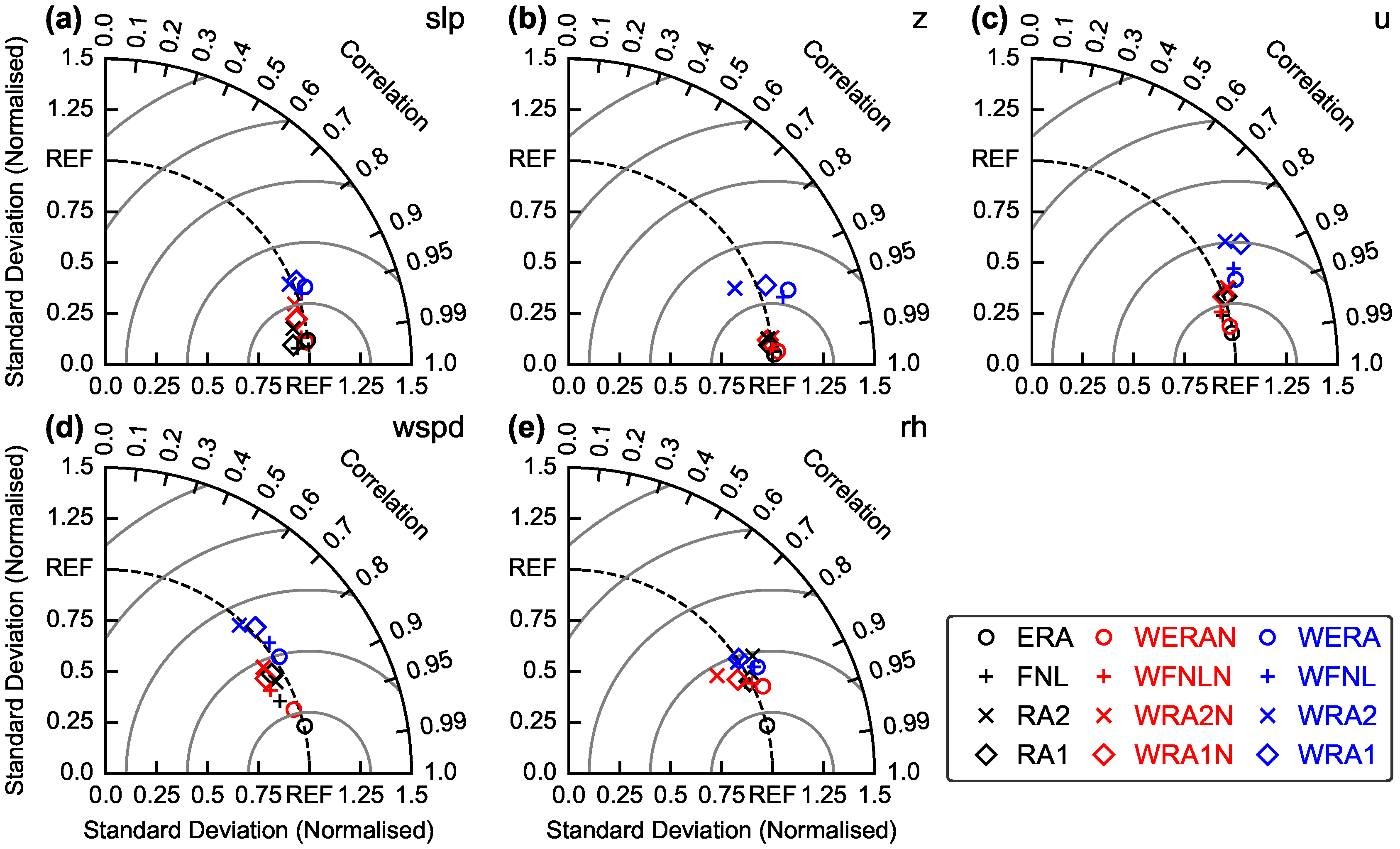
Figure 2a–e shows Taylor diagrams [
62] for the respective parameters on a daily basis.
The Taylor diagrams offer the possibility to display visually the statistical relationships between the WRF cases and the ILBCs with the reference data in terms of the correlation coefficient (
r) and the ratio of the standard deviations (
). They are defined by:
and:
with
M as the modeled value,
O as the observed value, as well as
and
as the respective standard deviations. For z and slp, the mentioned area averages were used, while for u, wspd, and rh, the vertical patterns were correlated. Basically, for all parameters, the WRF cases matched the spatio-temporal patterns of ERA5 quite well. However, there was a clear signal with respect to the spectral nudging technique. In each of the parameters, the WRF cases omitting nudging can be distinguished due to lower
r values. Especially, u and wspd showed this behavior. While WRA2 scored
r and
of 0.84 and 1.5, WERAN achieved values of 0.98 and 1.1, respectively (
Figure 2c). The highest scores were received for z and slp with
and
r close to unity for the nudging cases. For rh, the differences between the ILBC specification were less pronounced since this parameter was not nudged. However, an improvement in
r for the nudging cases can be recognized for WERAN and WFNLN. The smallest
of 0.82 was obtained for the WRA1 case, which indicates lower variability in rh than ERA5.
The corresponding biases for the austral summer and winter seasons are summarized in
Table 2. The bias is calculated by:
with
M as the model value and
O as the observed value.
Nearly all experiments and ILBCs showed positive biases in DJF. The strongest deviations occurred in the ERA cases, likely due to the already strong differences between ERA and ERA5 (13.8 hPa). Except for the simulations driven by FNL, spectral nudging produced a stronger pronounced anticyclone. In the case of the Chaco low region, the seasonal biases revealed that in most simulations, a stronger low pressure system was developed when driving WRF in the traditional long-term integration mode. The strongest deviation with 35.4 hPa was generated in the WRA2 experiment, while WERA exhibited similar slp intensities compared to the reference (0.8 hPa). The mean absolute differences in wspd for DJF were 1.2 m for the WRF cases omitting nudging and 1.0 m for the nudging cases. The highest positive bias was produced by WFNLN (0.6 m ) and the highest negative bias by WRA2 (−1.2 m ). During JJA, the deviations in wspd were higher with an absolute mean deviation of 3.3 m for the WRF cases running with spectral nudging, 4.0 m for cases running without nudging, and 5.5 m among the driving fields. Likewise in DJF, the strongest bias was produced by WRA1 (4.0 m ), and WFNLN scored best (0.4 m ). With respect to the vertical moisture distribution based on rh, all data revealed wetter (drier) conditions during DJF (JJA) than ERA5 in the ITCZ region. Again, the strongest improvement (lowest biases) generally was generated by simulations using spectral nudging, but with differences between the ILBCs.
Finally, the spatial patterns of the aforementioned features are illustrated in
Figure 3 and
Figure 4 for selected cases only.
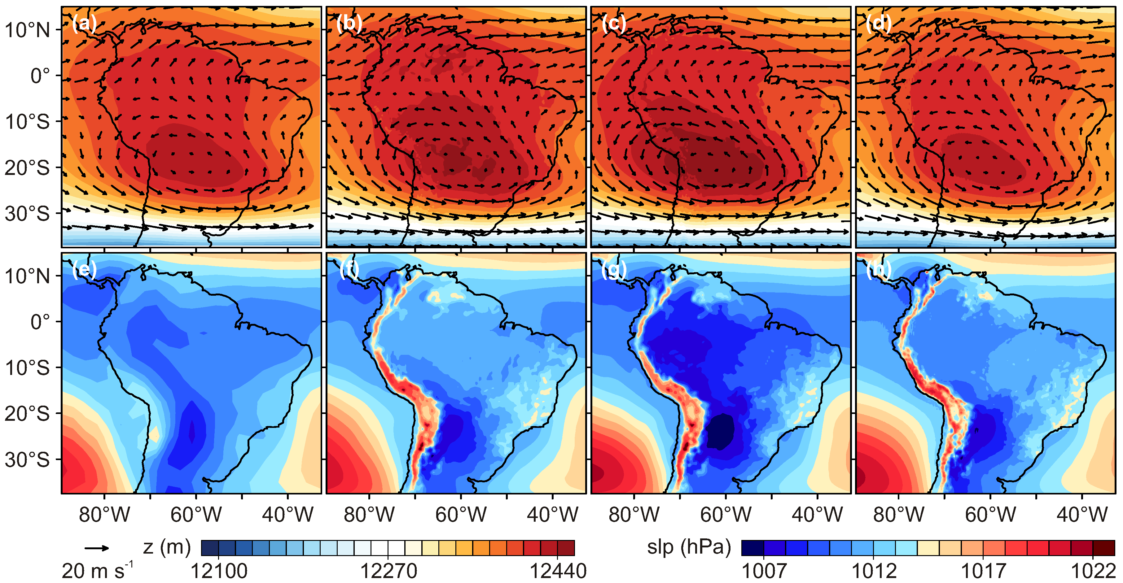
Figure 4a–d shows the upper-level (200 hPa) large-scale circulation (uv-wind vectors, m
) and z (shaded, m) for DJF of ERA, WERAN, WERA, and ERA5. As expected from the Taylor diagram and the biases, the simulations resembled the controlling features with the anticyclonic vortex centered over 20° S and 60° W, consistent with ERA5 and the driving fields. The southerly extension of the high pressure system, as well as the meandering structure of the westerlies forced by the anticyclone were well captured. During the austral winter months (JJA), the displacement of the BH and the northward shift of the westerlies were reproduced by the experiments (not shown).
As well as for the upper-level circulation the main slp patterns including the near equatorial trough and the thermal low pressure system over the La Plata region (i.e., Chaco low) are reproduced by each experiment. Near the south-eastern coast of Brazil and over the Andes Mountains complex slp patterns can be recognized as a result of the improved representation of the terrain in the RCM. Particularly noteworthy are the lower slp values in the Amazon basin as well as in the region of the Chaco low (
Figure 4g) compared to the corresponding forcing data and ERA5 (
Figure 4h).
Based on u and wspd, the development of the easterlies during DJF and JJA was demonstrated (
Figure 4). In both seasons, the WRF simulations resembled the spatial patterns, but differed in their intensities, and thus, corroborated
,
, as well as the biases.
4. Influence of ILBC Specification on Precipitation Behavior
The performance of the precipitation behavior is considered to assess model uncertainties according to the different ILBCs. A prominent feature representing precipitation in tropical South America is the ITCZ and its seasonal oscillation, as described above.
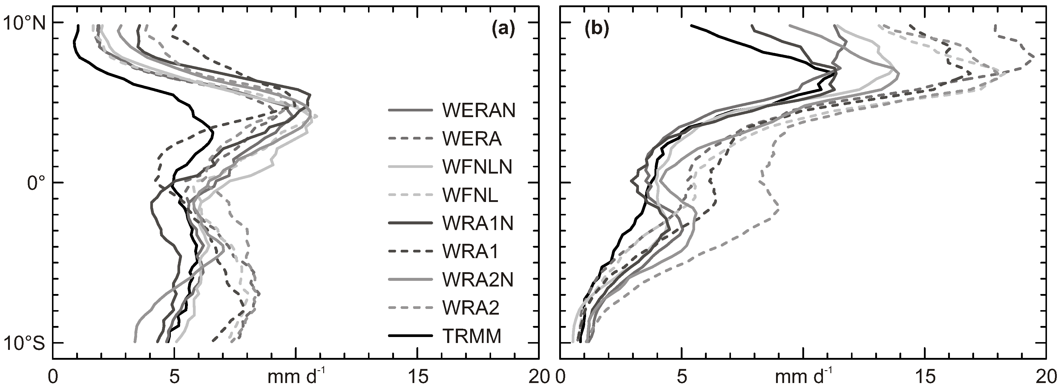
Figure 5 presents meridional profiles of daily precipitation for DJF and JJA with TRMM as the reference. The precipitation is zonally averaged between 70° W and 30° W to encompass the rainfalls over the Amazon basin. On the basis of the rain peaks around 4° N (DJF) and 6° N (JJA), the location of the ITCZ can be identified. In comparison to TRMM, the experiments captured both the locations and migration of the ITCZ, as indicated by the varying rain peaks. However, during DJF, a slightly more northward position, as well as greater magnitudes characterizing overestimation of rain within the ITCZ can be recognized. This may explain the negative biases in rh (
Table 2), consistent between the simulations. Further south, the degree of mismatch for the cases applying spectral nudging was smaller, which became even clearer during austral winter. The location of the ITCZ is well reproduced with WERAN, especially in DJF, as well as WRA1N (JJA), generating the most comparable zonally-averaged precipitation regimes.
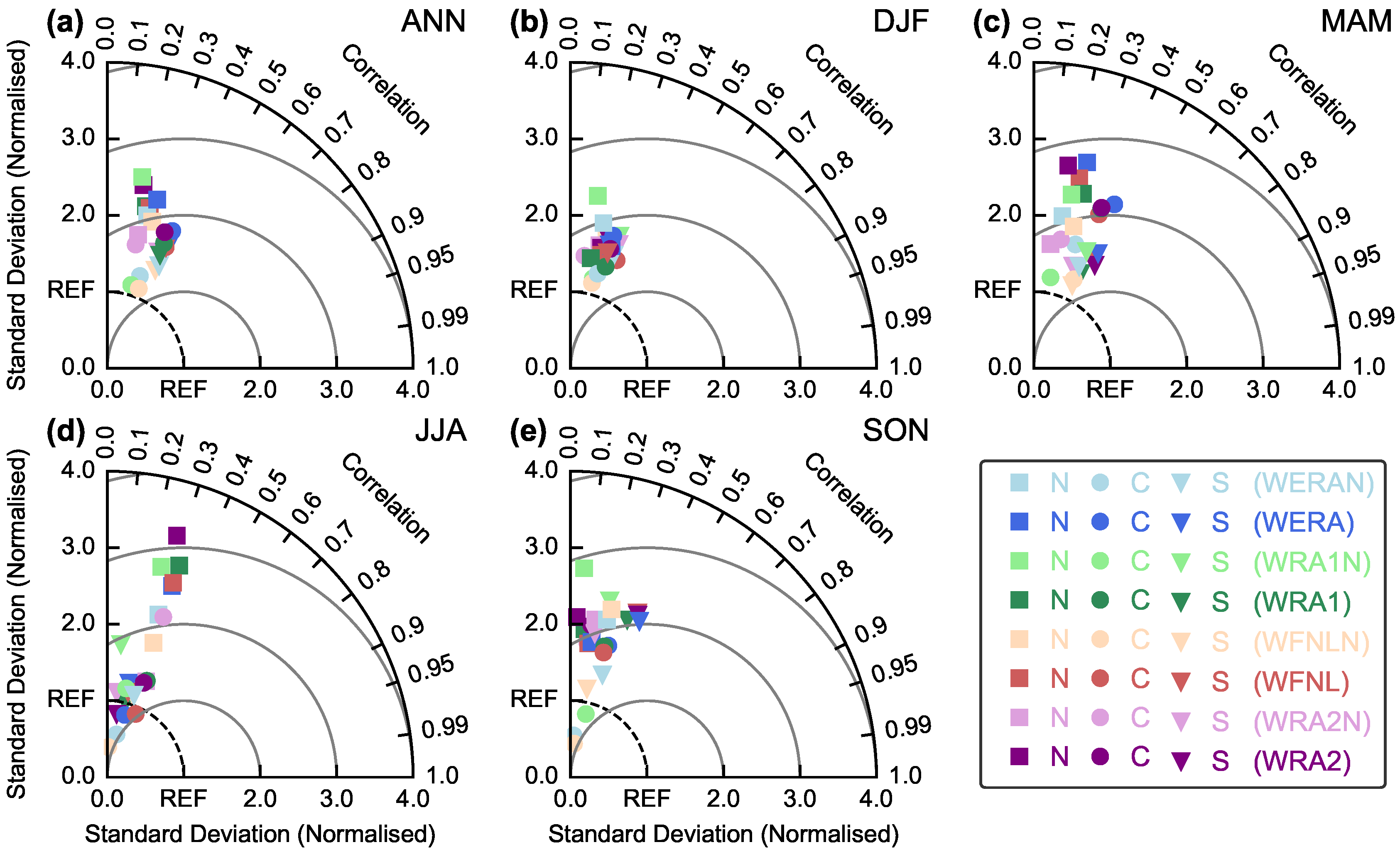
To examine the spatio-temporal consistency, as well as the over-/underestimation of rainfalls in the Andes highlands, Taylor diagrams on a seasonal basis were used.
Figure 6 shows the performance of the WRF simulations against TRMM for each subregion. Generally, the simulations revealed an overestimation of the precipitation, except for JJA and SON, but with clear differences between the regions. Featured by
, the largest wet (dry) biases emerged in the northern (central) subregion. Particularly during JJA and MAM, an overestimation in Subregion N can be noticed, reflecting the differently-acting driving features along the Andes range. While during JJA, the central and southern regions experience their dry season with strong westerlies blocking the eastern air masses, the easterlies are strongest in the northern Andes. The eastern air masses impinge the terrain and induce enhanced precipitation, which obviously result in stronger orographic rainfalls compared to TRMM, as indicated by
up to 3.2 (WRA2). In contrast, the smallest differences between the simulations can be observed in DJF, and the highest correlation is achieved in the southern Andes (S), particularly in the transitional seasons (March–May (MAM), September–November (SON)). Here,
r values of 0.5 were obtained for Subregions C and S. With respect to the ILBC specification, most of the experiments applying spectral nudging showed the best agreement with TRMM in both
r and
.
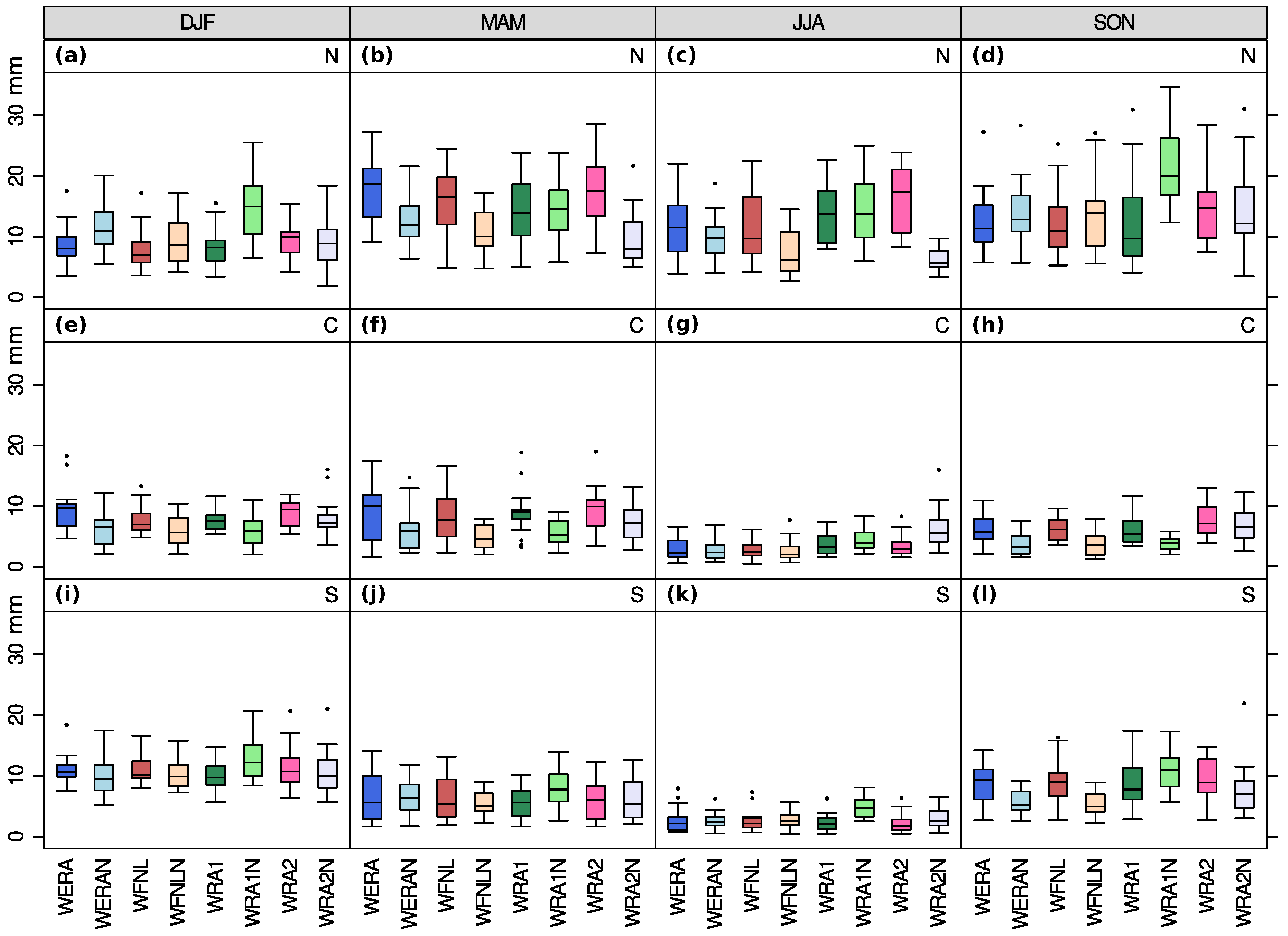
With the focus on the spatial distribution of the WRF precipitation over the three subregions within the Andes Mountains,
Figure 7 illustrates the root mean square error (RMSE) with TRMM as the reference on the basis of box plots. The RMSE gives additional information on the average magnitude of the model error and is calculated by:
with
M as the model value and
O as the observed value.
Here, we see not only differences between the ILBC specification, but also regarding the meridional location of the subregion and, thus again, the varying impacts of the large-scale features including seasonality. The best performance throughout the seasons was obtained in the central location (C,
Figure 7e–h) with a median RMSE not higher than 10 mm, while highest values occurred in the north (median RMSE up to 20 mm,
Figure 7a–d). On a seasonal basis, further differences are revealed. While Subregions C and S demonstrated their lowest RMSEs during JJA (
Figure 7g,k), Subregion N was most successful in DJF (
Figure 7a). This shift occurred due to the seasonal cycle in the large-scale atmospheric features and its varying influences along the Andes. Generally, the seasonality is less pronounced near the Equator. Thus, in the northern Andes in JJA, strong rainfalls develop due to the prevailing easterlies, while further south, it is the main dry season when the SPH strengthens. Across the regions, the selection of the forcing data also produced a clear signal in the uncertainty with a general low uncertainty using the ERA reanalysis. Interestingly, WRA1N showed the lowest interquartile range during SON in the central region (
Figure 7h), but the largest in the northern (
Figure 7d). Regarding the LBC specification, nearly all cases applying spectral nudging most successfully matched the spatio-temporal patterns of TRMM and presented a lower spread in the magnitude, as indicated by the smaller interquartile range.
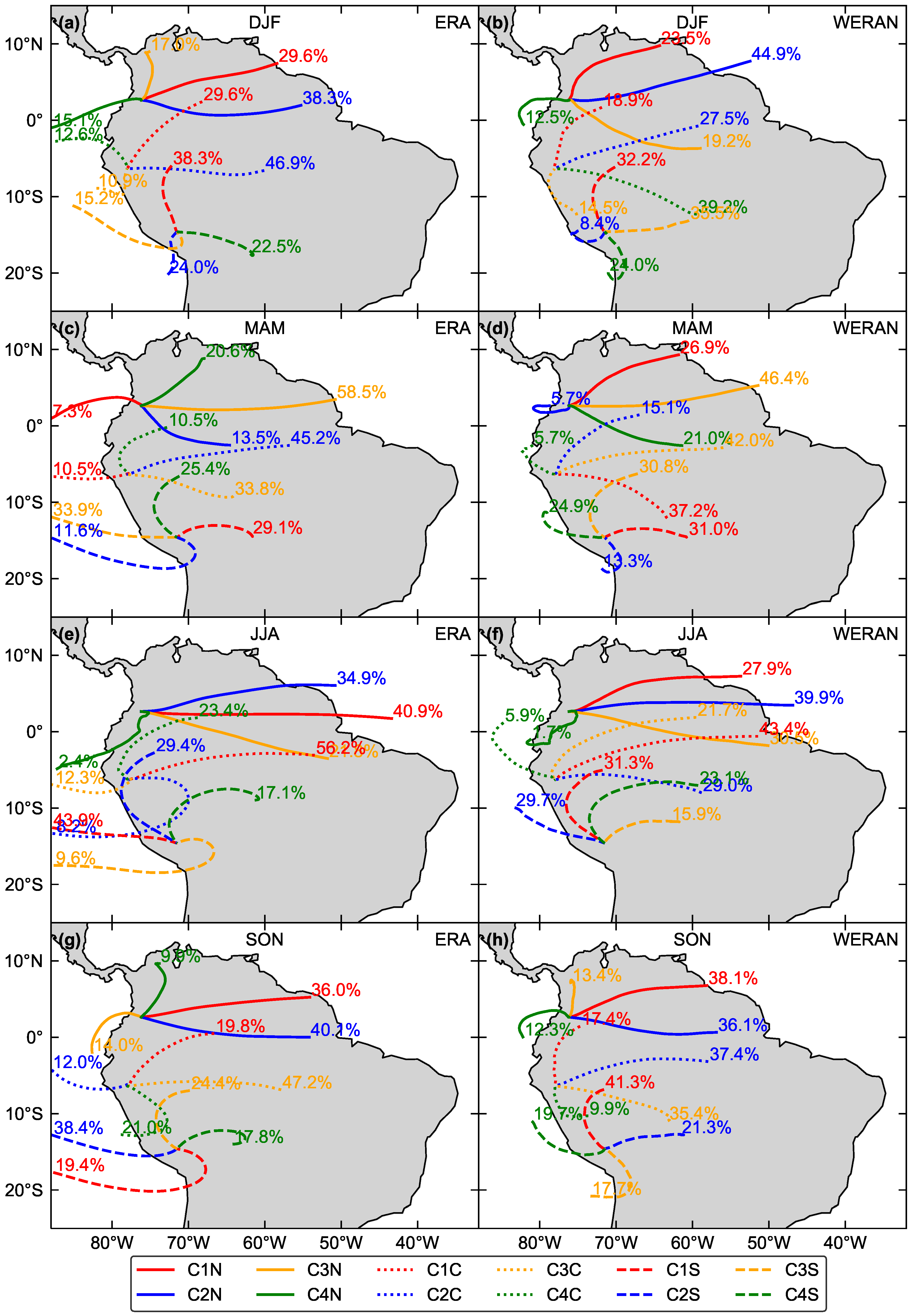
5. Atmospheric Moisture Pathways
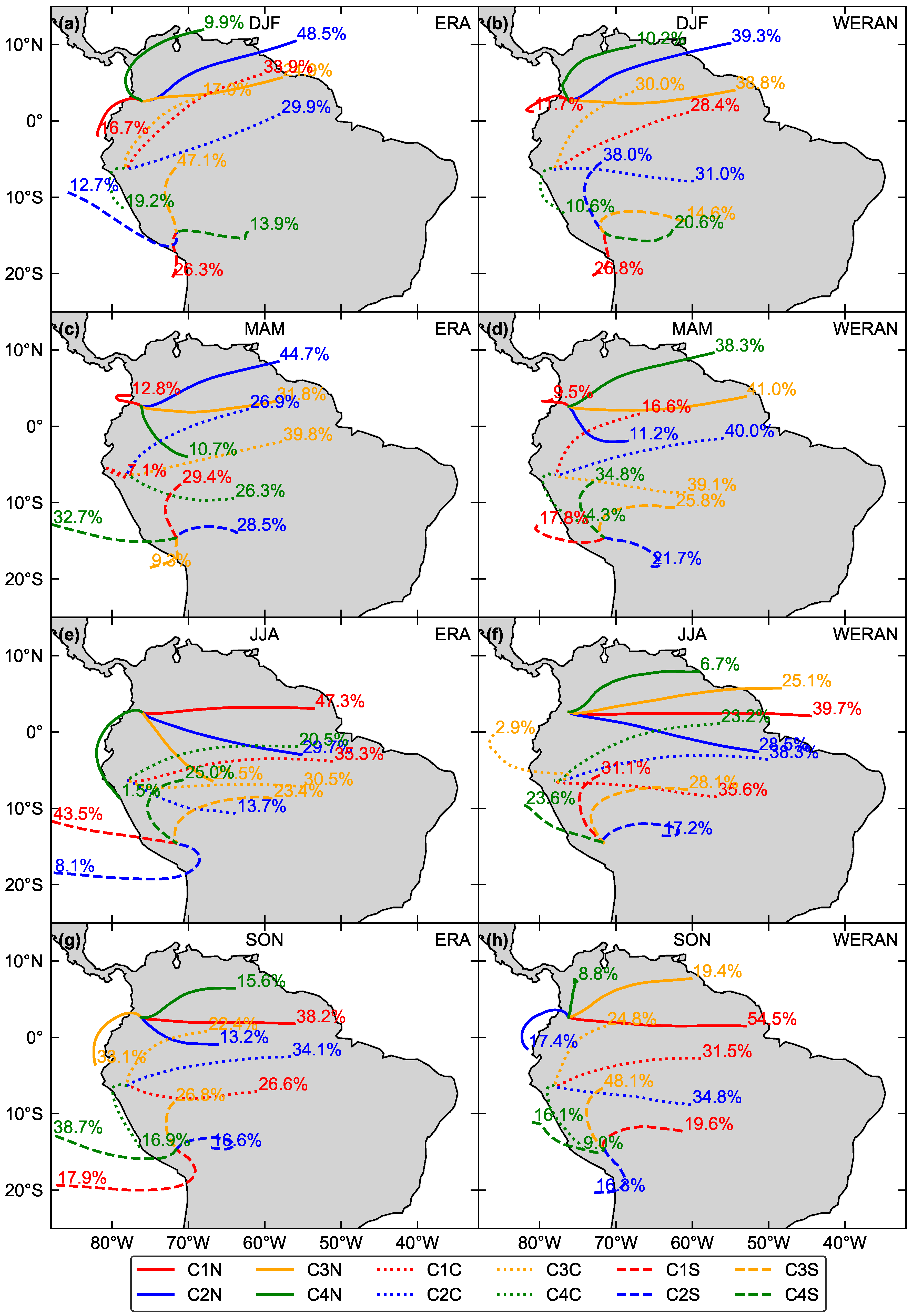
For the analysis of the atmospheric moisture pathways to the inter-Andean montane regions,
Figure 8 and
Figure 9 illustrate the representative air mass transport pathways obtained from the spherical clustering of the back-trajectories over all three years at the starting levels of 500 m agl and 6300 m asl, respectively. Here, only WERAN was analyzed as the simulation with the least uncertainty, as demonstrated in the previous section. To assess the added value of the downscaling procedure, the forcing data (ERA) are illustrated, as well. The dominant air mass trajectory clusters are displayed on a seasonal basis, since the large-scale atmospheric circulation is driven by a strong seasonal cycle. Overall, regardless of the height level, most of the trajectories pass over continental areas, which means that most of the moisture reaching the Andes highlands originates over the Amazon basin. However, westerly trajectories also evolve, although this is less frequent and obviously slower flowing, as indicated by the shorter pathways. Especially over coastal areas, the trajectories feature a bow-shaped pathway (except for JJA in Subregion N), which represents coastal wind systems associated with the Peru current in Subregion N, also described by Makowski Giannoni et al. [
50], and the SPH in Subregion C and S).
Regarding the meridional gradient of the subregions, clear differences in the marine air mass contribution can be recognized. In the southern subregion, Pacific air masses have a clear proportion on the atmospheric moisture transport into the highlands, which follows the seasonal changes in the large-scale dynamics. When the BH is weakened during JJA (
Figure 8e,f/
Figure 9e,f), one-third of the trajectories has a Pacific origin (24%/30%, Cluster C4S/Cluster C2S). This percentage increases when the ITCZ is shifted southward and the BH strengthens, as revealed by 26%/32% (DJF, Cluster C1S/Clusters C2S, C4S), as well as 32%/38% (SON, Cluster C2S, C4S/Cluster C3S, C4S). However, to a lesser extent, the northern subregion illustrates a comparable behavior with most of the air mass trajectories emerging over the Pacific coast during DJF (12%/13%, Cluster C1N/Cluster C4N) and SON (17%/12%, Cluster C2N/Cluster C4N). In contrast, the central subregion is dominated by fast flowing easterly air mass trajectories during all seasons. Only in JJA, a westerly moisture transport occurs, as described by Cluster C3C/C4C (
Figure 8f/
Figure 9f).
Comparisons to the trajectories obtained from the ERA forcing fields (
Figure 8b,d,f,h and
Figure 9b,d,f,h) display similar patterns with dominating transport pathways over the Amazon basin towards the Andes highlands. However, the western air masses represented by the WRF simulation are clearly less developed throughout the starting heights, the subregions and the seasons. Particularly within the PBL, ERA exhibits longer and, thus, faster moving air masses due to less adequately represented terrain compared to WERAN.
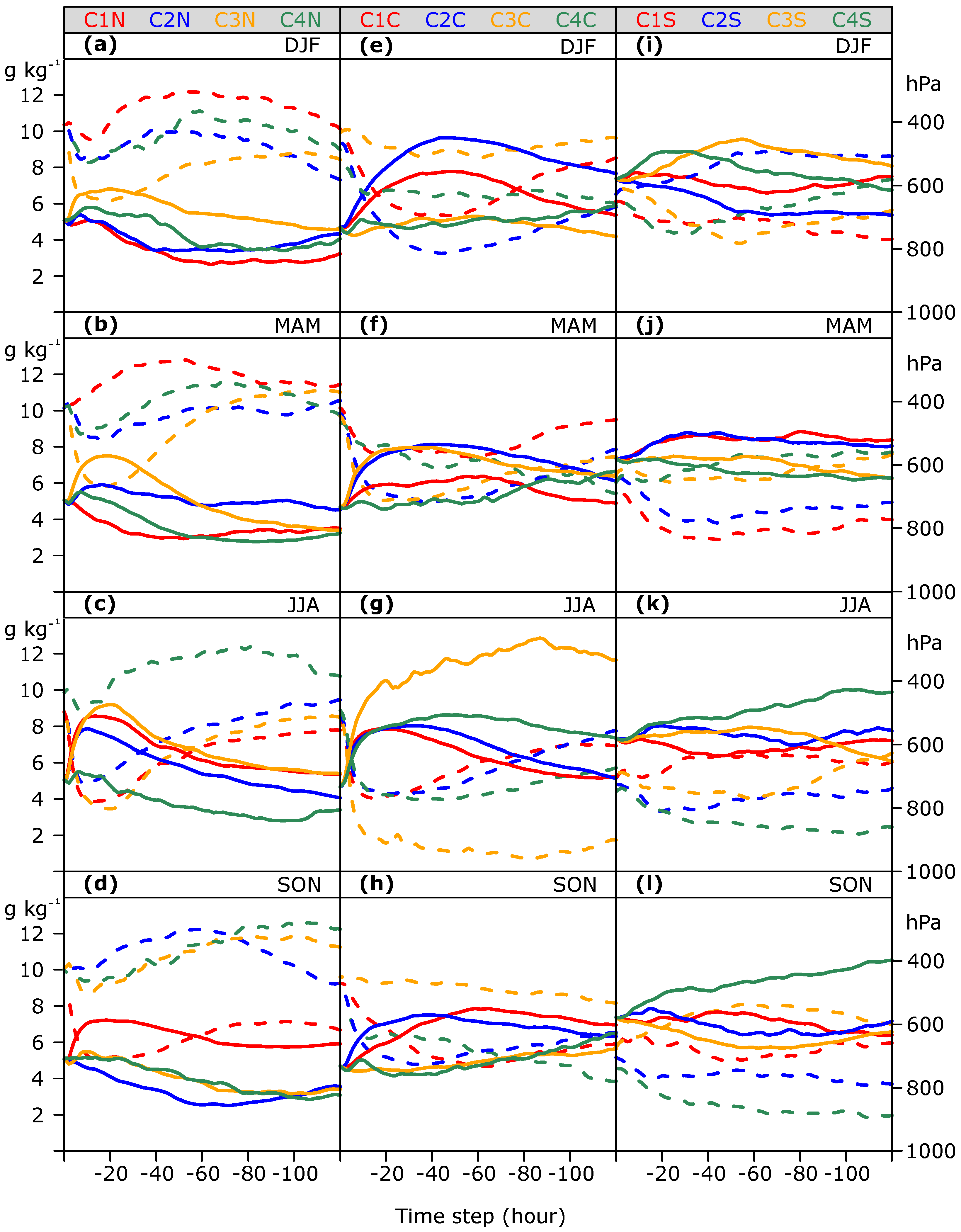
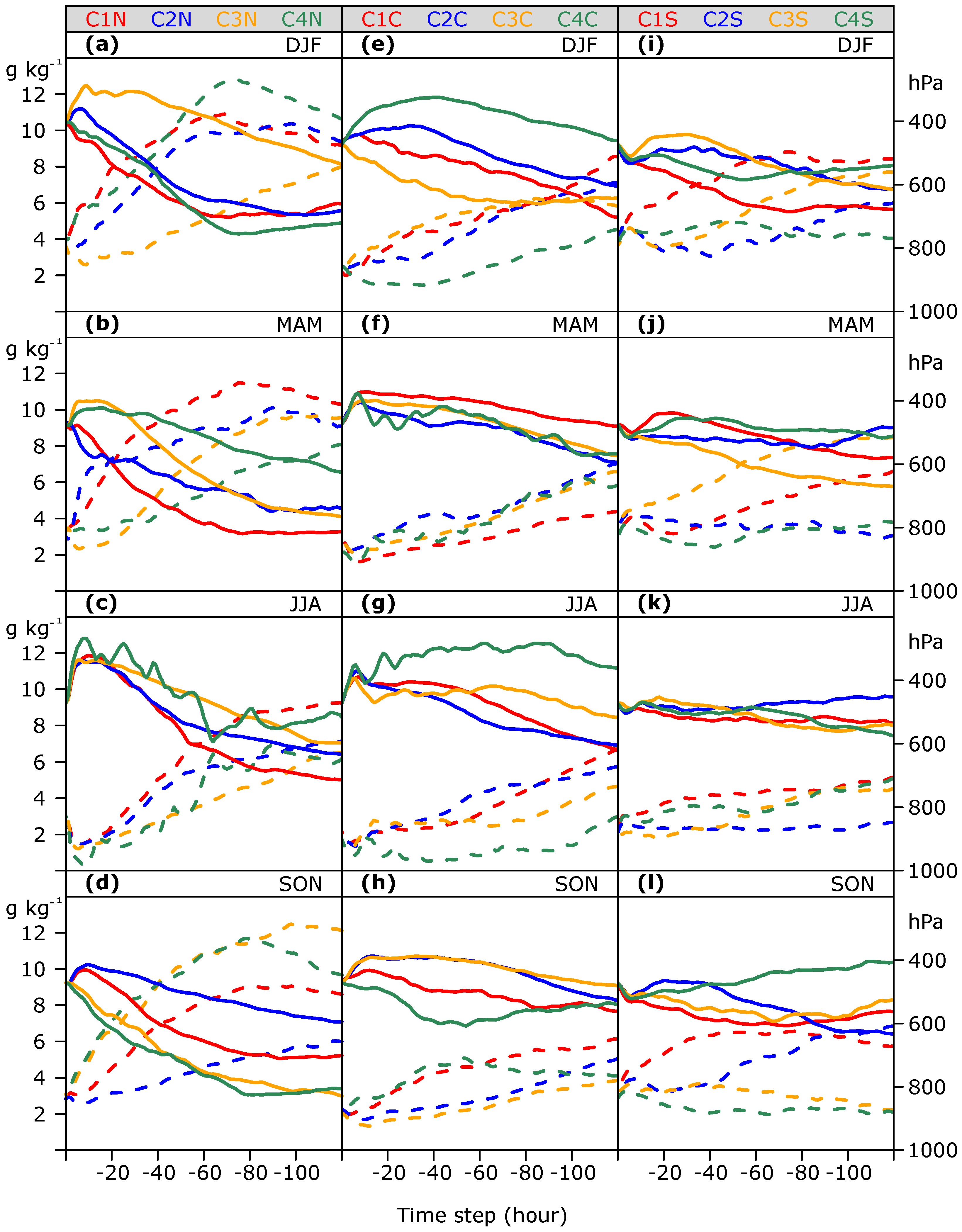
The contribution of each mean cluster trajectory to the moisture content over the three subregions is depicted in
Figure 10 (500-m agl starting level) and
Figure 11 (6300-m asl starting level) by means of the qv mixing ratio (g
, dashed line), as well as the pressure level (hPa, solid line) along the respective trajectory of WERAN. The qv mixing ratio obtained at the receptor sites (starting points of both levels) of each subregion is additionally summarized in
Table 3.
Generally, the trajectories revealed a rapid decrease in the pressure height level as they reached the Andean range, and qv correspondingly decreased. This points to forced lifting of air masses accompanied by orographic-induced rainfalls typically developing at the eastern slopes, but also at the western flanks above the inversion layer. Further, a clear relation between the height level and the qv mixing ratio can be observed, where lower traveling trajectories are accompanied by higher qv values and vice versa. As expected, the eastern transport pathways account for a large portion of the moisture availability in the Andean highlands with clear seasonal variations in its strength. The subregions mainly receive the moisture from the Atlantic, as well as the Amazon basin as the trajectories passes these regions. However, westerly trajectories originating over the Pacific Ocean also contribute to the atmospheric moisture in the highlands, as indicated by qv (
Table 3). This is particularly true in Subregion N (
Figure 10a–d and
Figure 11a–d), where compared to the other regions, the highest values occurred. Nevertheless, except in JJA, the western pathways of the 500-m agl level offer the highest amount of qv (10.36, 10.33 and 10.06 g
) at the receptor site among the mean cluster trajectories. In Subregion C (
Figure 10e,f,h), where nearly all trajectories have a continental origin, the bow-shaped pathways in DJF (C4C,
Figure 10e) and JJA (C3C/C4C,
Figure 10g/
Figure 11g) likely enable the uptake of Pacific air masses, also depicted in the slight peak in qv near the receptor site.
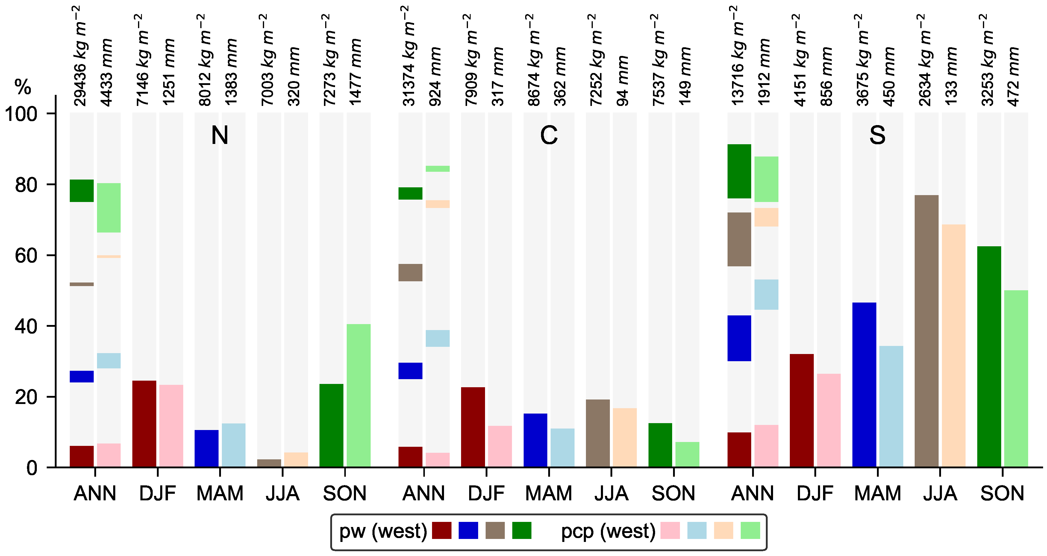
To assess the contribution of the westerly air mass transport on the moisture total column precipitable water (pw, kg
), as well as precipitation amount in the highlands,
Figure 12 illustrates their percentage fraction for each subregion on an annual and seasonal basis.
It is evident that in Subregion C, the westerly air mass pathways play a minor role in the contribution to the total pw and precipitation amount throughout the seasons. This clearly contrasts with Subregion S. Especially during JJA and SON when the BH weakens, the total pw and the precipitation amount increases, while the mean air mass trajectories pass over the Pacific Ocean. At the same time, the easterlies strengthen in northern South America, which is reflected in the marginal proportion of the westerly trajectories in the other subregions. This is also expressed by the seasonal western fraction on the annual pw and precipitation (
Figure 12, ANN). Interestingly, here, we can detect a shift in the seasonal proportions between pw and precipitation throughout the subregions. The seasonal fractions of pw are evenly distributed, whereas precipitation describes a distinct seasonality with a larger (smaller) fraction in SON (JJA).
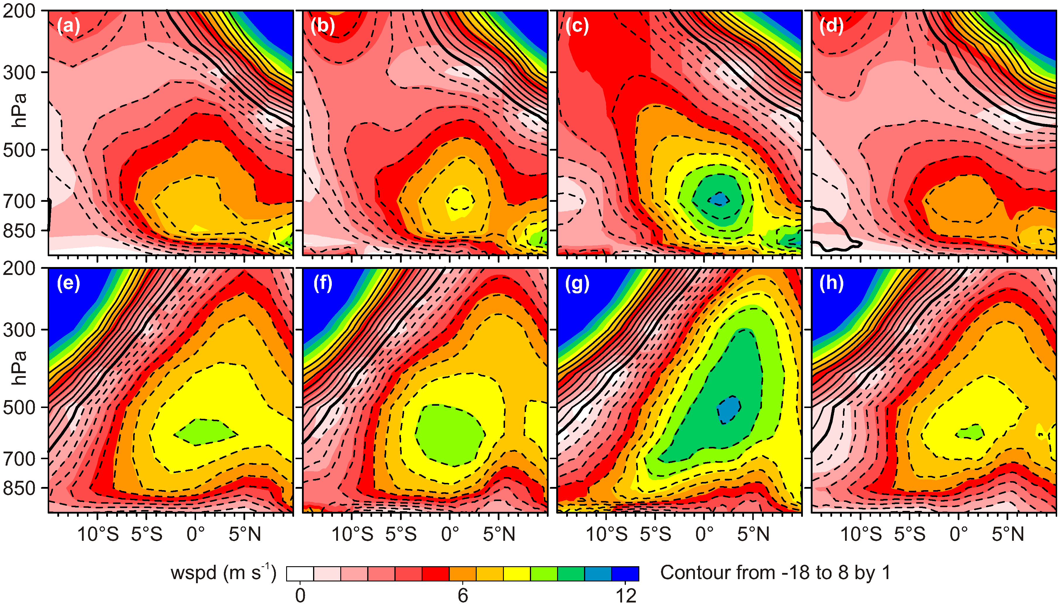
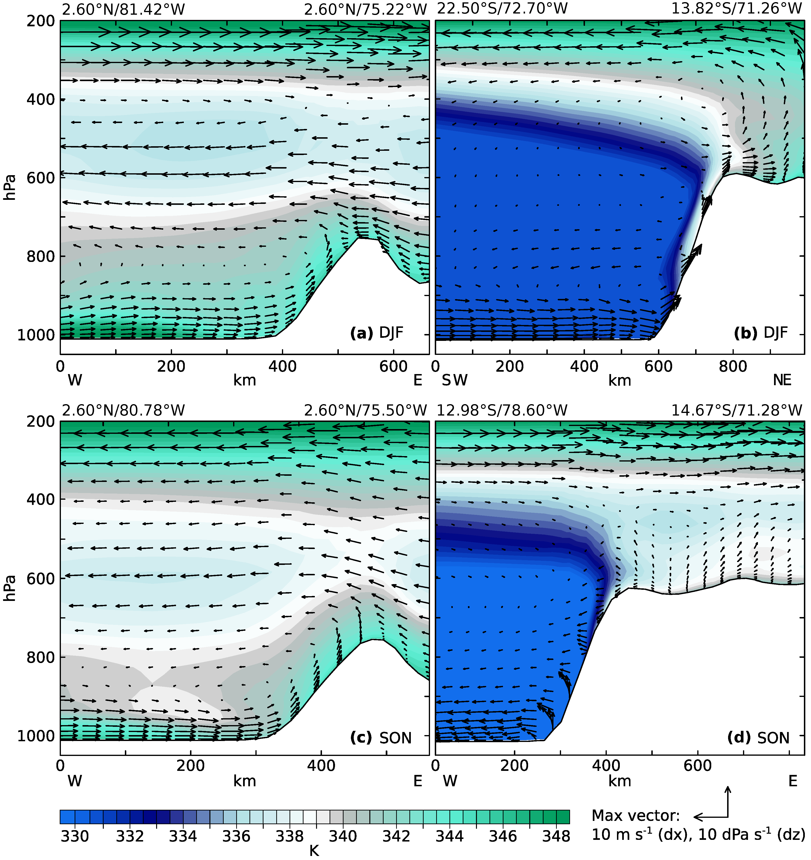
Since the atmospheric transport pathways are calculated for the PBL, as well as for the 400-hPa level,
Figure 13 illustrates cross-sections through the main region of the westerly mean cluster trajectories (calculated over the three years) of Subregion N and S (
Figure 8 and
Figure 9) during DJF (C1N/C4N, C1S/C4S) and SON (C2N/C4N, C4S/C1S). The seasons are used because of the highest percentage in the northern subregion illustrated in
Figure 10 and
Figure 11. The moisture and energy content of the atmosphere, as well as the flow regime are analyzed in terms of the equivalent potential temperature (
, K) and the wind vectors in uw directions (m
).
is quasi-conserved within an air mass, where the air is maintained at saturation by evaporation or condensation, and is defined by:
with
as the potential temperature,
as the latent heat of evaporation,
the specific heat content,
the temperature at the lifting condensation level (LCL), and
the mixing ratio for water vapor. The atmospheric conditions are averaged on a seasonal basis with respect to all time steps in which westerly back-trajectories emerged.
The vertical cross-sections reflect the meridional and zonal gradient in the distribution of moisture and energy affected by the prevailing flow regimes. During austral summer, an onshore flow near surface develops in the northern subregion (
Figure 13a,c). These sea-breezes advance warm-moist air masses to the western slopes indicated by
between 344 and 348 K. In the mid-troposphere, the easterly trade winds passing over the Andes can be observed. This layer features colder
down to 336 K, characterizing drier conditions, and thus, an inversion layer that is slightly stronger in DJF. Nevertheless, despite the persistent easterlies, slightly downward mixing of moist air from the upper-troposphere can be detected over the Andes ridge. In contrast, coastal air masses in the southern subregion are controlled by a strong inversion layer caused by the SPH (
Figure 1). Here,
below 330 K appear up to a height level of approximately 400 hPa. While in Subregion N, the conditions between the seasons differ in terms of their strength, Subregion S revealed comparable equivalent potential temperatures, but opposing flow regimes. In DJF, a near surface onshore wind arises with a transport of moist air masses into the western slopes, as well as an upper-level eastern flow, and vice versa. However, in both seasons, the downward mixing from air masses aloft can be recognized, which indicates the contribution of moisture from the Pacific Ocean. This entrainment is less pronounced in SON as the BH weakens.
6. Discussion and Conclusions
In this study, the atmospheric moisture pathways to the highlands of the Andes Mountains are examined using WRF simulations and HYSPLIT back-trajectories. As discussed in previous studies [
1,
13], deforestation and climate warming have strong impacts on the evapotranspiration over the Amazon basin and, thus, the sensitive hydro-climatic system in the Amazon-Andes transition. Using water vapor tracking methods, Agudelo et al. [
1] reported on changes in the recycling of water related to alterations in the evapotranspiration and highlighted the importance of understanding the role of regional circulation on the water vapor transport.
In order to gain the most accurate regional circulation patterns associated with the atmospheric transport pathways, spectral nudging was tested against traditional long-term integration using four different ILBCs with varying horizontal resolutions. As described by Bowden et al. [
26] and Solman and Pessacg [
25], an accurate representation of the driving large-scale fields helps with reducing and understanding the appearance of small-scale biases.
Based on the Taylor diagrams (
Figure 2a–e), the benefit of spectral nudging was illustrated, as deviations to the reference (ERA5) decreased in these experiments, consistent with previous studies [
27,
31,
33]. On the other hand, the simulations forced with the traditional long-term integration were characterized by lower
r values for each parameter, as well as a clear signal in
by means of greater differences in the variability than the reference data (ERA5). Thus, it is very likely that the flow developed within the model becomes inconsistent with the driving fields. Moreover, using spectral nudging reduced systematic errors in the synoptic fields, as well as produced stronger correspondence with the reference data (ERA5). With respect to the parameters and characteristics considered, an improvement of the simulation results could be observed without constraining the models’ ability to evolve small-scale variations, as demonstrated in
Figure 3 and
Figure 4, lacking in the ILBC, consistent with Liu et al. [
33]. Since only long waves above the PBL were nudged, the model was allowed to develop its own variability freely [
29,
30], which points to a sufficient degree of freedom of WRF.
Concerning the atmospheric features (BH, Chaco low and ITCZ), their spatio-temporal variability was well reproduced by each experiment and in good agreement with ERA5 (
Table 2,
Figure 2,
Figure 3 and
Figure 4). This may not be surprising since they are dominated by the large-scale forcing ILBCs. However, differences in the ILBC specification, which mainly appeared in terms of their intensities rather than their location, could be recognized. In turn, these deviations affect the moisture pathways through stronger gradients associated with higher wind speeds and, thus, faster traveling air masses. Special attention was given to the development of the lower-level convergence zone based on the easterly jet and the moisture transport (
Figure 4), since the seasonal course of the ITCZ affects the climate variability along the Andes chain according to the moisture advection [
8]. The inter-hemispherical shift was generated regardless of the forcing data, but distinct discrepancies in the intensities of the easterly jet could be noticed. In particular, when driving WRF in the long-term integration mode, stronger velocities (8–9 m
against 11 m
) were generated, which in turn influenced the moisture pathways, as well as the location of their sources.
In addition, precipitation as an important part of the hydro-climatic system was used to further assess model uncertainties concerning the ILBCs. Over the Amazon basin (
Figure 5), the seasonal mean precipitation profile representing the ITCZ revealed a greater agreement to TRMM for the experiments applying spectral nudging. Both the intensity and the location of the precipitation peak, i.e., the ITCZ, were better represented in these simulations. Precipitation over the Andes Mountains was generally featured by an overestimation, which is characteristic for challenging areas such as complex terrain. Nevertheless, the results of the spectral nudging cases indicated a greater consistency with TRMM, but with clear variations between the three subregions and the seasons (
Figure 6 and
Figure 7). These alterations reflect the varying influences of the large-scale atmospheric circulation along the Andes chain. In particular, Subregion N demonstrated evident wet biases in JJA. During these months, the ITCZ shifts to the Northern Hemisphere and the trade winds have a strong eastern component. Subsequently, an orographic enhancement of precipitation develops as the easterlies converge with the terrain, which leads to the overestimation. This was also observed by means of the RMSE (
Figure 7). In contrast, the lowest RMSE could be identified in the southernmost subregion (S) during austral winter, when the BH is weakened. Regarding the ILBC, experiments with spectral nudging generally disclosed a better performance likely due to lower wind speeds and more accurate moisture conditions, as noted by the biases and Taylor diagrams (
Table 2,
Figure 2).
The results of the mean cluster trajectories for both height levels (
Figure 8 and
Figure 9) confirmed the predominance of the eastern pathways. However, following the seasonal oscillation of the large-scale features and the meridional location of the receptor sites, western trajectories also play a role in the transport of moisture to the Andean highlands. This conclusion was further corroborated by the qv mixing ratios related to the air mass pathways (
Figure 10 and
Figure 11,
Table 3).
Especially during MAM and SON, Pacific air masses frequently occurred in Subregion S with a clear contribution to the moisture content over the Andes highlands. In this region, the Pacific trajectories revealed a large amount of moisture, although qv in comparison to the inner tropical regions had lower mixing ratios (4.4–6.13 g
and 2.1–3.73 g
). During JJA, as the SPH strengthens and the ITCZ is located further north west, pathways were mostly blocked in the northern Andes, except for the 6300-m asl level (C2N, MAM) (
Figure 9). Nonetheless, these trajectories had a low frequency of occurrences (6%) contrasting with C2S (JJA, 30%), which is under the influence of anticyclonic conditions, as indicated by the northwestern wind direction. Comparing the mean cluster trajectories of WERAN and ERA, it is evident that most of the pathways mainly differed in their length, which means higher wind speeds in the coarser resolved data. With respect to each individual year (
Figures S1 and S2), the mean cluster trajectories showed similar atmospheric transport pathways, which pointed to the robustness of the results.
The seasonal percentage amount of the total column precipitable water pw and precipitation obtained from WERAN during westerly air mass trajectories reflected these conclusions (
Figure 12). Mainly in Subregion S, the Pacific trajectories likely contributed to the total amount of pw and precipitation, whereas in Subregion C, the western air masses played a negligible role. In the northern Andes, the percentage of pw and precipitation during western wind directions is clearly related to the location of the ITCZ, associated with the strength of the eastern trade winds. With respect to the annual cycle, the seasonal percentages disclosed that during DJF and JJA, the fractional distribution of precipitation changed compared to pw. This indicates that further processes such as the stratification of the atmosphere have an effect on precipitation and, thus, on the recycling of moisture. In JJA, precipitation was only produced in Subregion S during the western trajectory episodes. Moreover, in Subregion C, the proportion of pw is evenly distributed over the seasons, which is not true for precipitation. The seasonal percentage of precipitation in JJA is clearly lower, probably due to the stable stratification related to the SPH.
In order to gain insights into the atmospheric conditions and underlying dynamics throughout the atmosphere, cross-sections of
and the wind vectors through the regions of the cluster trajectories of both levels, i.e., C1N/C4N and C1S/C4S (DJF), as well as C2N/C4N and C4S/C1S (SON), were used (
Figure 13). The results highlighted the vertical moisture and energy distribution during the western events and exposed that moisture was advanced to the Andes by slope breezes, as well as entrainment from the air aloft. Subregion N demonstrated a conditionally unstable layer near the surface (
) with an onshore flow regime that transports moisture to the highlands. In the mid-troposphere, colder
values could be recognized (335 K), which decoupled the air aloft. Nevertheless, over the ridge, this layer was discontinued, which divided the western and eastern air masses. Associated with westerlies aloft, entrainment from Pacific air masses emerged. In Subregion S, the atmospheric conditions, and thus the moisture transport, are rather dominated by the inversion layer over the coastal areas. Large-scale subsidence associated with the SPH caused stable environmental conditions, as indicated by
. However, despite this strong inversion layer, anabatic winds developed and advanced the warm-moist marine air to the highlands. This is particularly true for DJF (
Figure 13b), as the SPH is located further south (
Figure 1a) and a coastal jet along the Peruvian coast clearly evolved. As reported by, e.g., Trachte et al. [
48], a low-level south-western onshore wind over the Pacific Ocean produces strong land-sea breezes and the uplift of the moisture-laden air masses. On the other hand, during SON, descending air masses were aloft, and an offshore wind direction predominated. However, in both seasons, downward mixing of warm-moist air masses appeared and contributed to the moisture content in the Andes highlands, which seems to be affected by mid- and upper-level flow regimes [
11].
As shown, spectral nudging and the choice of the driving fields have clear effects on the precipitation behavior and the leading atmospheric moisture pathways. Applying spectral nudging generally produced a higher agreement to the reference data (ERA5). Concluding from the mean cluster trajectories and the qv mixing ratios, atmospheric pathways originating over the Pacific also contributed to the moisture availability in the high Andes Mountains, primarily in the southern subregion. Differences in both the meridional location of the receptor site and the season mainly occurred due to the seasonal oscillations of the large-scale atmospheric features controlling the moisture transport. In the northern Andes, the prevailing easterlies determined the occurrences of Pacific air masses, while in the southern subregion, the state of the BH is most relevant. These relations are especially true in non-anomalous situations related to ENSO, but modified in anomalous events [
63,
64]. Since there are complex interacting dynamics driving the atmospheric moisture transport in the tropical Andes highlands, further analyses are needed to encompass ENSO-related events.


