
Adaptive Surface Modeling of Soil Properties in Complex Landforms

1
School of Geography, Geomatics and Planning, Jiangsu Normal University, Xuzhou 221116, China
2
School of Environment Science and Spatial Information, China University of Mining and Technology, Xuzhou 221116, China
*
Authors to whom correspondence should be addressed.
ISPRS Int. J. Geo-Inf. 2017, 6(6), 178; https://doi.org/10.3390/ijgi6060178
Submission received: 24 April 2017
/
Revised: 16 June 2017
/
Accepted: 18 June 2017
/
Published: 20 June 2017
Abstract
:Spatial discontinuity often causes poor accuracy when a single model is used for the surface modeling of soil properties in complex geomorphic areas. Here we present a method for adaptive surface modeling of combined secondary variables to improve prediction accuracy during the interpolation of soil properties (ASM-SP). Using various secondary variables and multiple base interpolation models, ASM-SP was used to interpolate soil K+ in a typical complex geomorphic area (Qinghai Lake Basin, China). Five methods, including inverse distance weighting (IDW), ordinary kriging (OK), and OK combined with different secondary variables (e.g., OK-Landuse, OK-Geology, and OK-Soil), were used to validate the proposed method. The mean error (ME), mean absolute error (MAE), root mean square error (RMSE), mean relative error (MRE), and accuracy (AC) were used as evaluation indicators. Results showed that: (1) The OK interpolation result is spatially smooth and has a weak bull's-eye effect, and the IDW has a stronger ‘bull’s-eye’ effect, relatively. They both have obvious deficiencies in depicting spatial variability of soil K+. (2) The methods incorporating combinations of different secondary variables (e.g., ASM-SP, OK-Landuse, OK-Geology, and OK-Soil) were associated with lower estimation bias. Compared with IDW, OK, OK-Landuse, OK-Geology, and OK-Soil, the accuracy of ASM-SP increased by 13.63%, 10.85%, 9.98%, 8.32%, and 7.66%, respectively. Furthermore, ASM-SP was more stable, with lower MEs, MAEs, RMSEs, and MREs. (3) ASM-SP presents more details than others in the abrupt boundary, which can render the result consistent with the true secondary variables. In conclusion, ASM-SP can not only consider the nonlinear relationship between secondary variables and soil properties, but can also adaptively combine the advantages of multiple models, which contributes to making the spatial interpolation of soil K+ more reasonable.
1. Introduction
Scientific management and utilization of soil resources is predicated on correct understanding of the continuous changes in regional soil properties. Spatial interpolation is the main method used to evaluate continuous changes in soil properties [1], as well as being an important research tool in the fields of ‘digital soil’ and ‘pedometrics’ mapping [2]. Current spatial interpolation methods mainly originate from discrete modern mathematical theories (function theory and differential geometry), and can be largely classified into three groups [3]: (1) deterministic or non-geostatistical methods (e.g., inverse distance weighting, IDW), (2) geostatistical methods (e.g., ordinary kriging, OK), and (3) combined methods (e.g., regression kriging). These methods are often data- or even variable-specific and their performance depends on many factors. No consistent findings have been acquired to identify the best interpolation method, and most are global models (i.e., the same model is applied over the whole study area) [4,5]. However, in areas of landform complexity, the spatial distribution of soil properties is affected by secondary variables such as soil type, land use type, and landform type, and it is difficult to satisfy the basic assumptions of current models [6,7]. Further, owing to various shortcomings, single interpolation models restrict the improvement of prediction accuracy.
In recent years, some machine learning methods have been applied to the fields of data mining and spatial interpolation and have demonstrated their predictive accuracy; for example, artificial neural networks (ANN), random forest (RF), and support vector machine (SVM). Furthermore, ANN and SVM have been applied to daily minimum air temperature and rainfall data in some subjects [8,9]. However, all of these represent global interpolation models, which are difficult to adapt to landform complexity areas. Utilizing the advantages of ensemble learning for regression, we combined a series of interpolation models to carry out interpolation simulation of the spatial variation in soil properties and verified the reliability of multi-model integration [10]. Despite this, issues still remain; for example, in previous work, we only conducted a global regression integration of various interpolation models, with limited consideration of discontinuous space and spatial variation problems. Furthermore, remaining interpolation models need improvement and optimization before they can be integrated.
In addition, a range of studies have demonstrated that interpolation accuracy and mapping quality can be effectively improved by the use of secondary variables as supplementary information [4,11,12,13,14,15,16,17,18]. Land use, soil type, grassland type, and geology type might be expected to play a significant auxiliary role in controlling the spatial variation of soil properties. Previous work by Shi et al. [1] demonstrated the effectiveness of incorporating land use type and soil type to improve interpolation simulation of soil properties. In addition, many studies have identified topography as an important auxiliary element [3,19], but previous research results suggest it is not a key factor in the study area [10]. Therefore, integration of secondary variables in this study should have an important influence on interpolation accuracy.
In order to solve the global model and secondary variable problems that had long troubled the interpolation method, this study aimed to address some of the outstanding issues, with an overall goal of improving the prediction accuracy of the single interpolation model in areas with complex landforms, using soil K+ as an example. We applied analysis of variance (ANOVA) to select secondary variables closely related to the spatial variation of soil K+, integrated secondary variables, and constructed a series of soil property interpolation models. To deal with the discontinuity and spatial variation of soil properties in areas with complex landforms, error surfaces were constructed to enable adaptive partitioning of interpolation surfaces for screening suitable base interpolation models. This paper optimized the screened base interpolation models, and built and coordinated multi-model integration interpolation methods (different combinations of interpolation models were selected for different areas) to realize a high precision simulation of soil properties. We evaluated the performance of the different spatial interpolation methods IDW, OK, OK-Landuse, OK-Geology, OK-Soil, and ASM-SP, and analyzed their predictive capabilities in terms of soil K+ maps.
2. Method
2.1. Study Area and Datasets
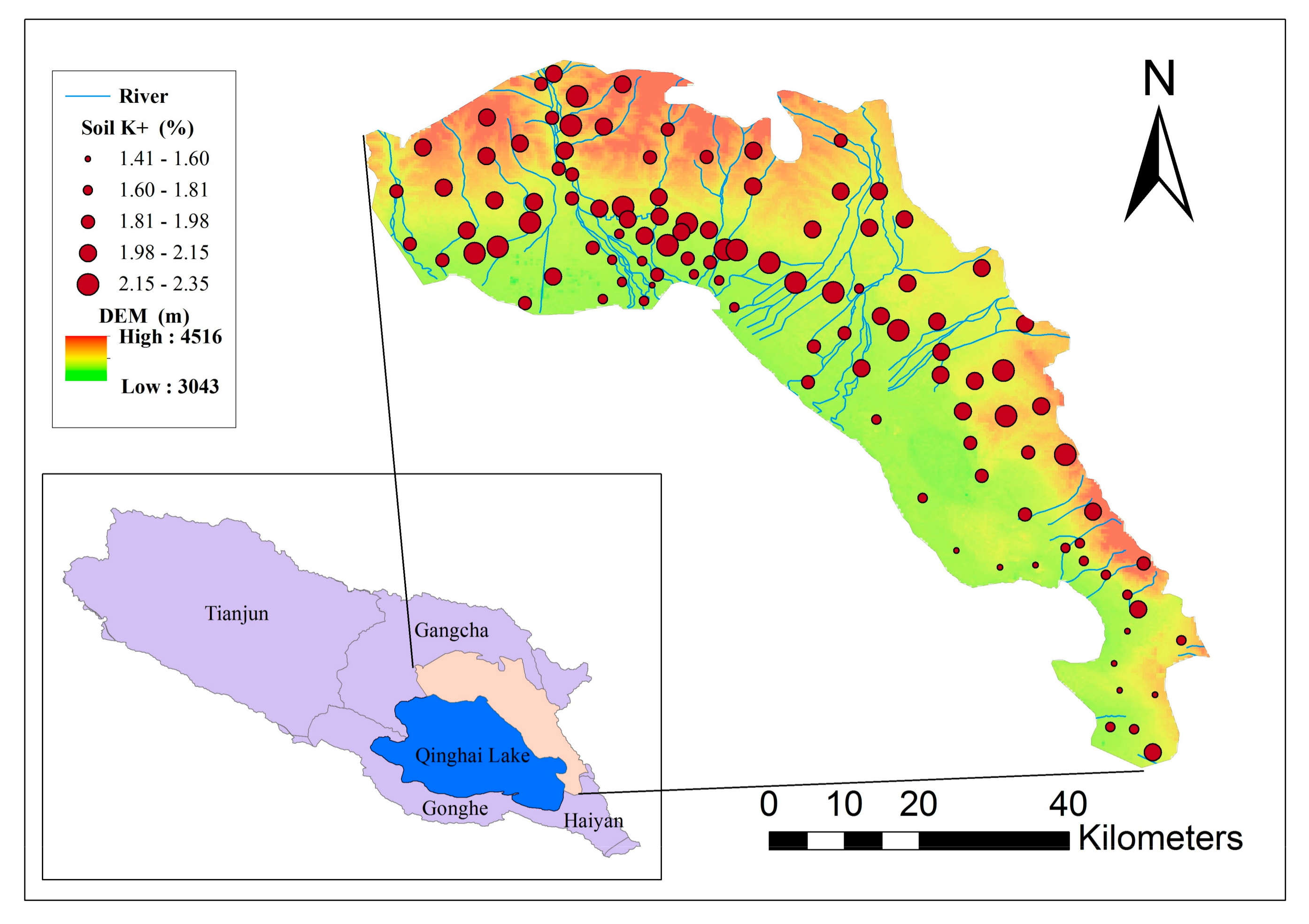
The study area (36°38′–37°29′ N, 99°52′–100°50′ E) is located in the southeast part of the Qinghai Lake Basin, on the Tibetan Plateau, China (Figure 1). The long-term combined action of geological movement and external forces have formed a complicated and diverse array of geomorphic features in the area. The study area covers a total of 2100 km2, with an altitude ranging between 3043 and 4516 m, and is characterized by complex landforms, including mountains, hills, tablelands, and plains. Abundant agricultural and husbandry activities are carried out in the area.
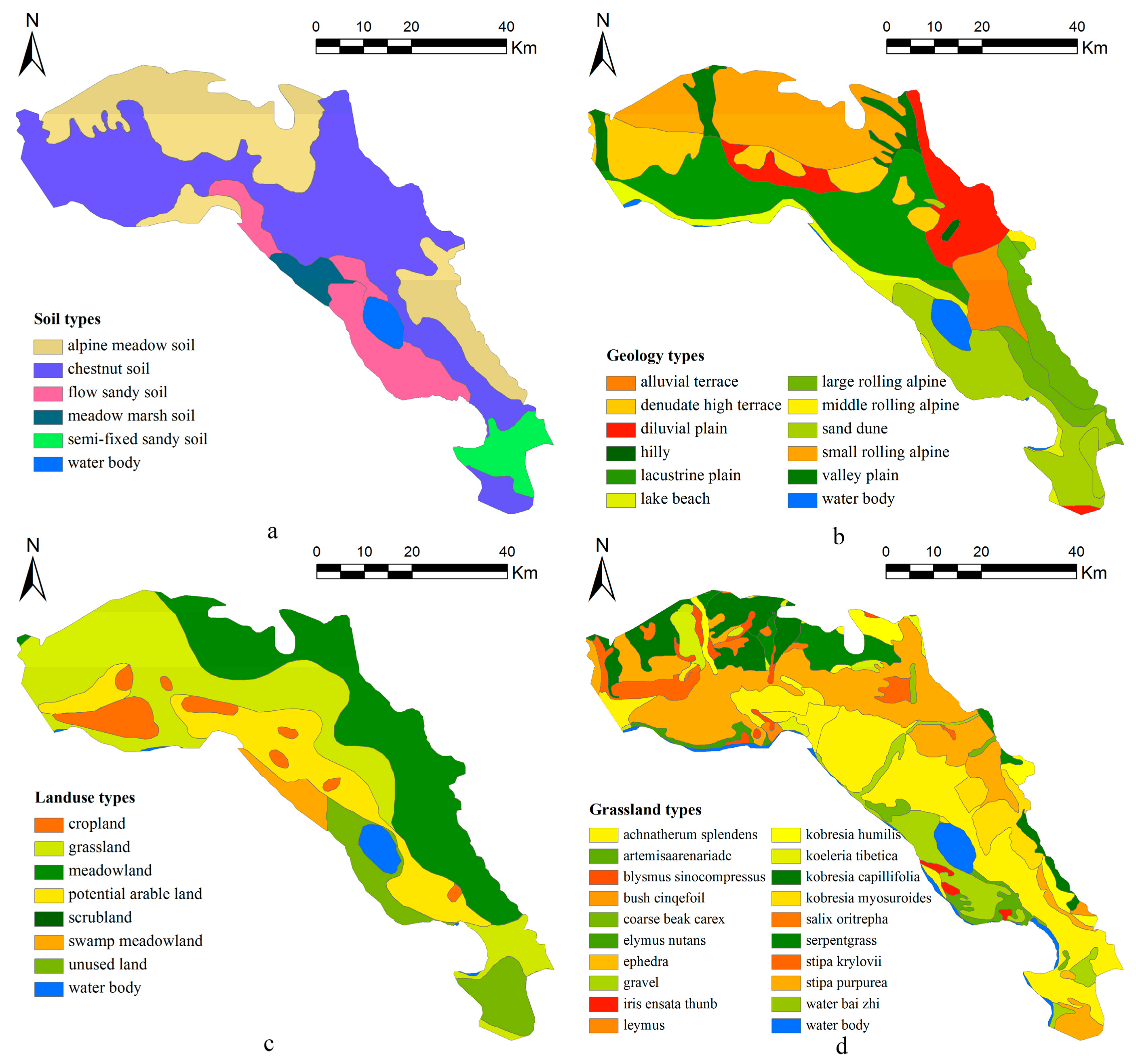
The study area is characterized by 6 soil types (Figure 2a); 12 geology types, including alluvial terrace, denudate high terrace, and diluvial plain (Figure 2b); and 8 land use types, including cropland, grassland, and potential arable land (Figure 2c). The grassland can be divided into 20 types, mainly including Achnatherum splendens, leymus, and Blysmus sinocompressus (Figure 2d). We calculated the statistical characteristics of soil K+ in secondary variables using 110 training samples (Table 1).
Field sampling of surface soil (0–30 cm) at 110 sampling points was carried out in September 2013 to supplement map data. The mean distance between soil sampling locations was approximately 6.74 km. The sampling sites were designed to cover the whole area and include different landscapes. In order to ensure rational distribution of the sampling points across the different geo-environments, a spatially stratified sampling strategy was applied based on landscape types [20]. Supported by the Qinghai Environmental Monitoring Center, we recorded information such as soil type, altitude, geology, and land use for each sample location. Each position was sampled three times and the mean was recorded as the sample value. Soil samples were taken back to the laboratory for analysis. After air drying, grinding, and screening through a 2 mm sieve, soil K+ of the samples was measured using sodium hydroxide melting analysis [21].
The secondary variables were compiled in ArcGIS 10.2, and converted to a resolution ratio of 30 m through resampling. Since the study area covers a comparatively large range of landscape types, and the number of samples was relatively small, the spatial distribution of samples was uneven (Figure 1) and some landscape types with a relatively high degree of fragmentation are poorly represented. In the study area, the subtypes of secondary variables not sampled anywhere covered only a very small area (i.e., scrubland; Figure 2c; Table 1). For this area, we directly used the nearest five-point surrounding values for the subtype to calculate the mean value.
2.2. Methods for Spatial Interpolation
2.2.1. Inverse Distance Weighting
IDW is a deterministic method for multivariate interpolation using a known scattered set of points. Values assigned to unknown points are calculated with a weighted average of the values available at known points. Weights are usually inversely proportional to the power of distance [22], which, at an unsampled location x, leads to an estimator:
where Z*(x) is the predicted value, Z (xi) is the measured value, n is the number of closest points (typically 10 to 30), p is a parameter (typically p = 2), and d is the cut-off distance.
2.2.2. Ordinary Kriging
Kriging interpolation is considered the best unbiased linear estimation method [23]. When the mathematical expectation of the regionalized variable Z*(x) is unknown, it is termed ordinary kriging. Z*(x), the estimated value of variables at point x, is obtained by the linear combination of n Z (xi)s, the effective observed value, using the expression:
where is the weight given to the observed value and represents the contribution of each observed value to the estimated value Z*(x). It can be calculated by the semi-variance function of the variables on the condition that the estimated value is unbiased and optimal. The semi-variance function can be expressed by the equation:
where is the semi-variance, N(h) is the point group number at distance h, is the numerical value at position , and is the numerical value at distance .
2.2.3. Base Interpolation Models
As a kind of geostatistical model [24,25], each observation z(xmn,ymn) of a specific soil K+ at location (x, y) in the n-th type of the m-th kind of secondary variable can be expressed as:
where m(Emn) is the mean value of z(xmn,ymn) in the n-th type of the m-th kind of secondary variable, and r(xmn,ymn) is the residual computed by subtracting the mean value m(Emn) of the n-th type of the relative m-th secondary variable from the measured value of soil K+. We assumed that m(Emn) and r(xmn,ymn) are mutually independent and that variation of r(xmn,ymn) is homogeneous over the entire study area. The residuals were then used to interpolate the surface of residuals over the whole study area by OK. Finally, the interpolated residual values were summed to the soil K+ means of the relevant secondary variable as the final interpolated values of OK with secondary variable for the soil K+; that is, the mean was modified with surface modeling of residuals. See Section 3.3.1 for the specific modeling process of base interpolation models (i.e., OK-Landuse, OK-Soil, OK-Geology).
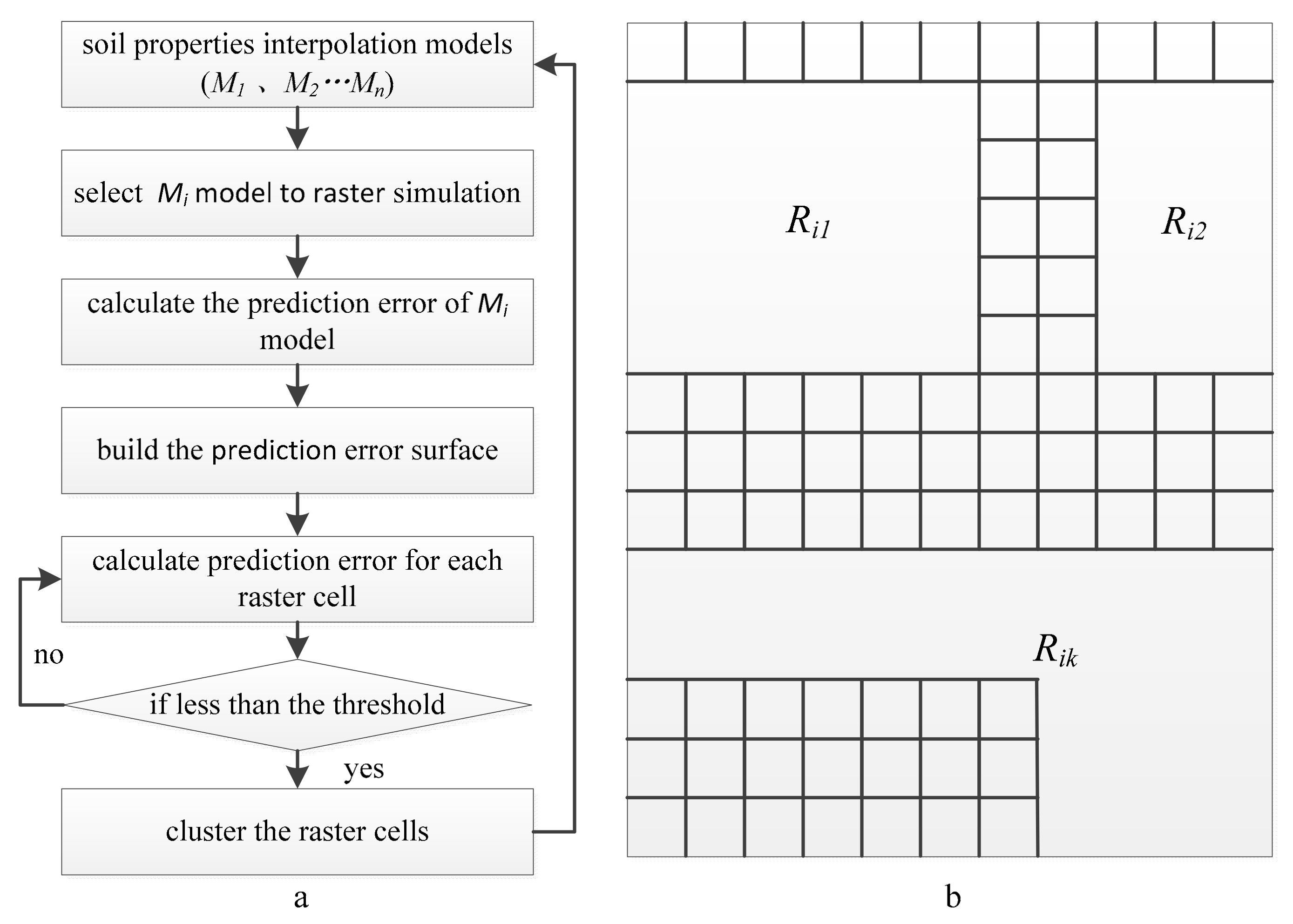
2.3. Method for Adaptive Partitioning
A series of interpolation surfaces of soil properties were generated from the base interpolation models to calculate simulation errors for soil sampling points. The error surface, derived from linear interpolation, was used to determine whether the error of each raster cell exceeded a threshold value. Raster cells below the threshold value were clustered to determine the spatial range of applicability of each interpolation model after multiple iterations. The individual steps are shown in Figure 3a and detailed below.
Step one: Raster cell simulation. For a specific soil property interpolation model (e.g., Mi), soil properties are calculated for the whole study area at a specific resolution ratio C0 to give the raster simulation value S0;
Step two: The soil property simulation error at each sampling point is calculated by subtracting the simulation value from the measured value;
Step three: Error surface construction. The error surface is constructed using linear interpolation based on the simulation error obtained in step two;
Step four: Calculate the simulation error of soil properties at each raster cell, based on the error surfaces obtained in step three;
Step five: Determine whether ei (i=1, 2, …m), the error of each raster cell, satisfies | ei | < ε, where ε is the error threshold. If it does, this raster cell is marked as a clustering cell;
Step six: Clustering. Areas that meet the accuracy threshold are clustered based on the spatial locations clustering cells. Ri1, Ri2, and Rik, etc., are the cluster spaces of the interpolation model Mi (Figure 3b);
Step seven: Repeat the above steps for each interpolation model to determine their applicable spatial ranges.
2.4. Assessment of Performance
Independent validation was applied to assess interpolation accuracy. The soil K+ sample data were randomly split into two groups, one of which was used for interpolation and the other for validation. A total of 90 soil K+ sample points were used for interpolation and the remaining 20 were used for validation.
We assessed the accuracy of the different interpolation methods by comparing the mean error (ME), mean absolute error (MAE), mean relative error (MRE), root mean square error (RMSE), and accuracy (AC) of predicted and measured values. The specific equations used are as follows:
where n is the number of samples; PEV is the potential error variance (PEV); and are the measured and predicted values, respectively; and is the mean measured value. AC varies between 0 and 1, with larger values indicating a better predicted result. Smaller values of ME, MAE and RMSE, indicate greater interpolation accuracy. MRE is dimensionless and smaller values indicate greater interpolation accuracy.
3. Results
3.1. Parameter Specification and Selection of Secondary Variables
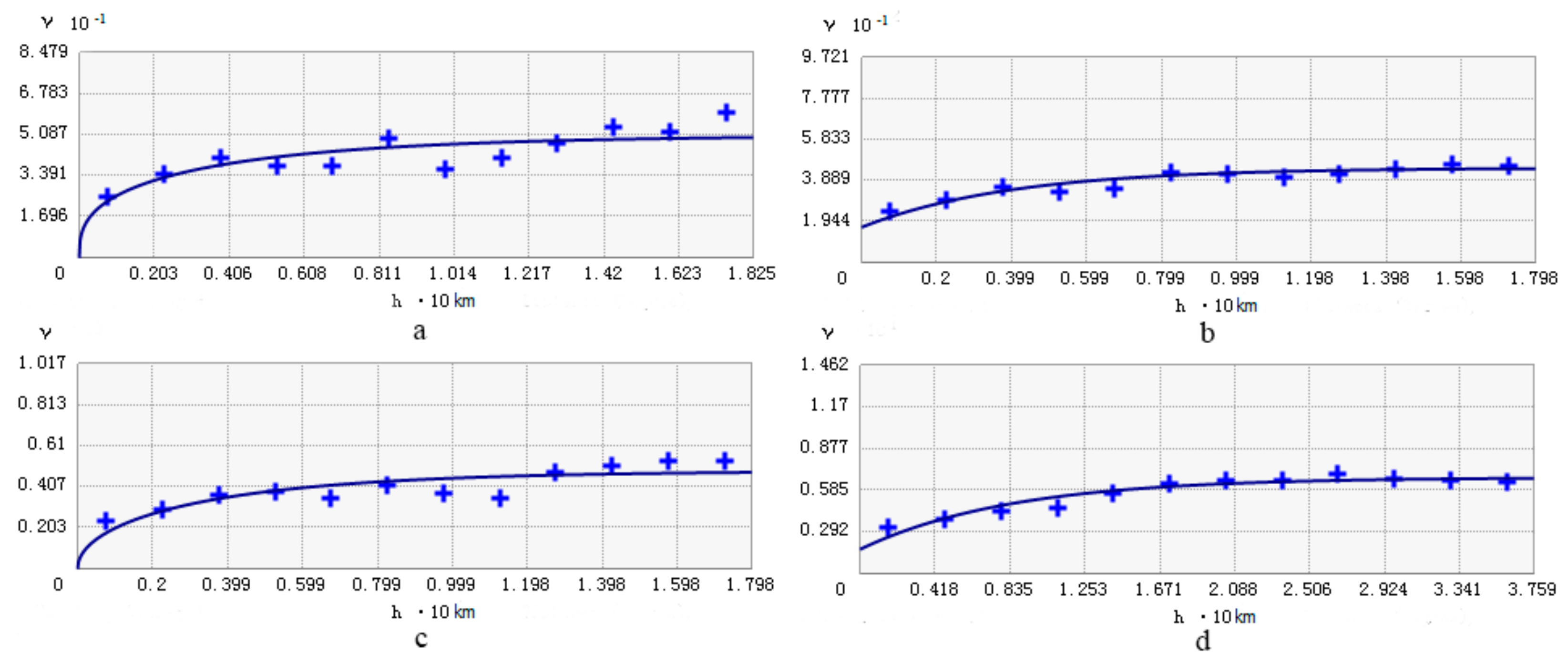
Based on fitted nugget, sill, and range values, the semi-variogram model was selected for analysis of spatial correlation. Other models were considered, including exponential, spherical, Bessel, circular, and Gaussian, while exponential and K-Bessel models were selected for the OK and base interpolation models as they better fitted the data/residuals (Figure 4). To determine the number of kriging samples, we chose the best samples from 5 to 30 at 5-step intervals.
The spatial correlation of residuals showed good performance after removal of the local mean within the different secondary variables (Table 2). All of the semi-variograms of residuals tended to show a smaller sill and a shorter range, indicating that drift had been removed [26]. The nugget/sill ratio (N/S) of residuals was <0.3 for all models except OK-Geology, which indicates strong spatial correlation of the residual data [27]; the spatial correlation increased after trend removal. This finding suggests that the OK and base interpolation models were appropriate for the study area.
The secondary variables used for each method were analyzed by ANOVA. The soil K+ data were grouped into classes in order to compare soil K+ for the different secondary variables. For example, in terms of soil type, the soil K+ data were grouped into five classes: alpine meadow soil, chestnut soil, flow sandy soil, meadow marsh soil, and semi-fixed sandy soil, with 32, 54, 10, 6, and 8 samples in each, respectively. The soil K+ variances between and within soil types were determined by ANOVA using SPSS 21.0 for Windows.
3.2. ANOVA Analysis of Soil Properties for Different Secondary Variables
The ANOVA results comparing the influence of different secondary variables on Soil K+ are shown in Table 3. Geology type, soil type, and land use type are strongly correlated with the spatial variation in soil K+, with significance at the 0.01 level. However, grassland type is poorly correlated with soil K+ (significance level of 0.2). This is mainly due to the larger degree of fragmentation of the soil map of grassland types, and the limited number of sample points for some grassland, with some subtypes of grassland having just 1 or 2 sampling points (Table 1). Hence, grassland type was not used in the process of constructing the base interpolation and ASM-SP models.
3.3. ASM-SP
The ASM-SP was constructed in three steps: first, a number of base interpolation models were produced (e.g., OK-Landuse, OK-Soil, and OK-Geology); second, the base interpolation models were partitioned by an adaptive method; third, the base interpolation models were combined using a popular combination scheme. The models OK-Landuse, OK-Soil, and OK-Geology were used as the base interpolation models. Adaptive partitioning was conducted on the base interpolation models using the method described in Section 2.3 to construct error surfaces; partitions that met the accuracy requirement were screened and the ASM-SP was constructed based on raster cell optimization. The specific steps were as follows.
3.3.1. Construction of Base Interpolation Models
Step one: Equation (4) was used to calculate mean soil K+ for each geological factor and obtain mean surface m(Emn). The mean soil K+ was correlated to the secondary variables, based on measured values of soil K+ (Figure 5).
Step two: The mean value of soil K+ was subtracted from the measured value to calculate the residuals of soil K+. The residuals were then interpolated by OK to obtain the residual surface r(xmn,ymn) (Figure 6).
3.3.2. Adaptive Partitioning of Interpolation Surfaces
Based on the method for constructing error surfaces outlined in Section 2.3, the local polynomial interpolation was used to obtain error surfaces for the different interpolation models (Figure 7) and to determine the spatial range of applicability for each interpolation model.
3.3.3. Integration of Interpolation Surfaces
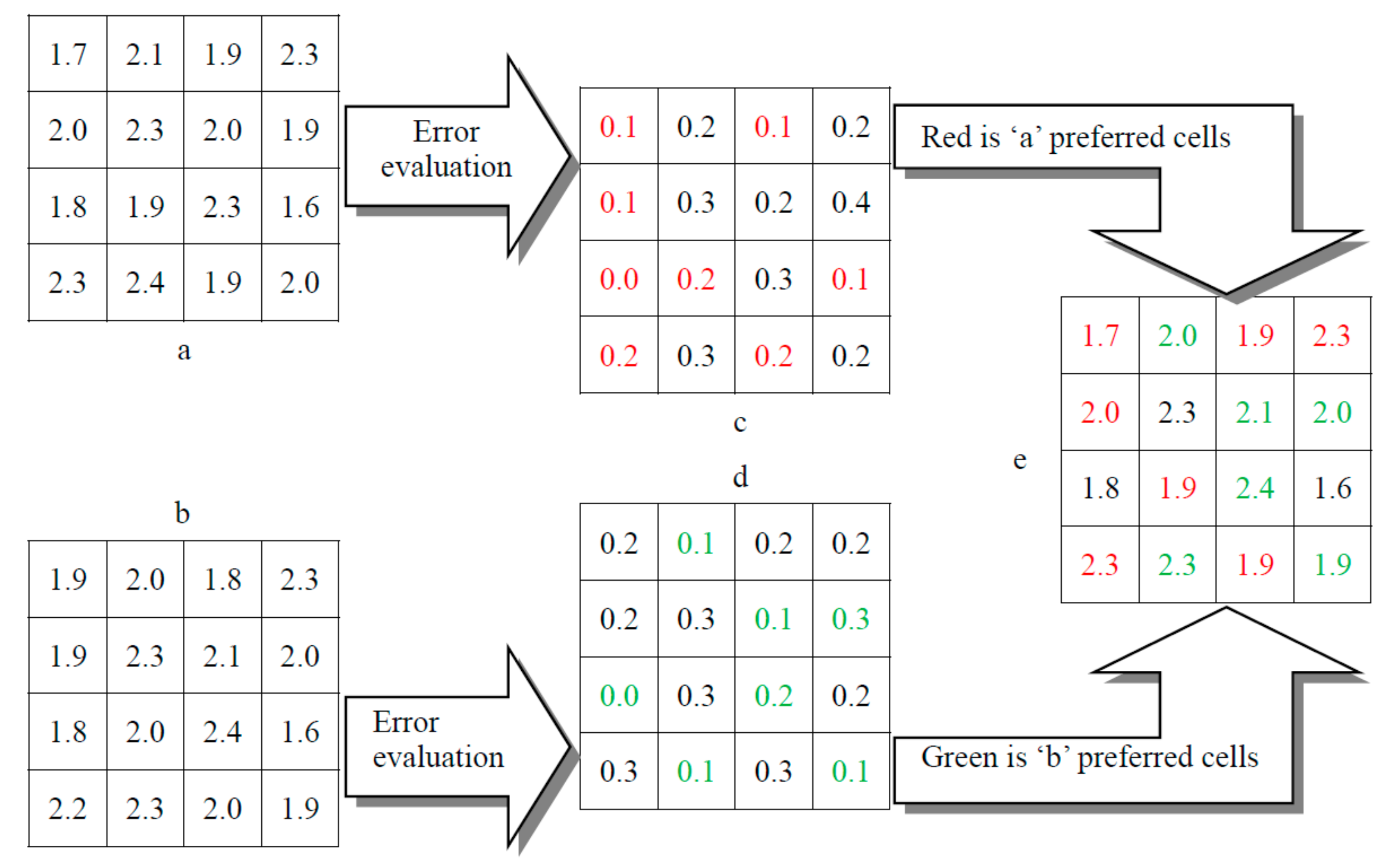
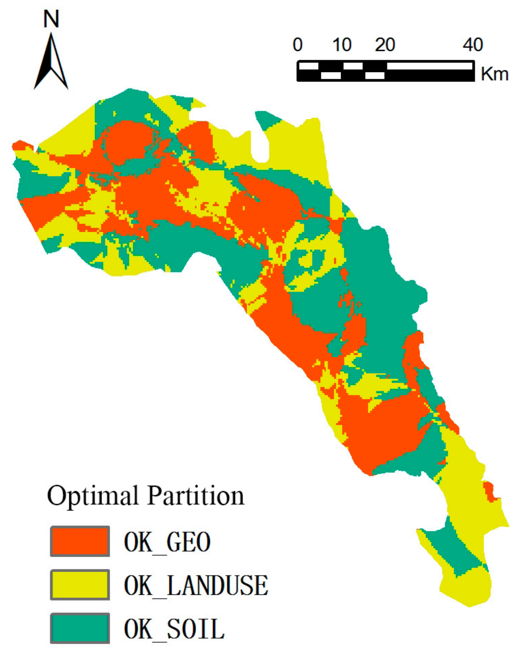
On the basis of raster cell optimization, interpolation results of raster cells with the minimum error were selected as the optimal raster cell to be integrated. Figure 8 displays the principle of the raster cell optimization method, and Figure 9 shows the optimal partitions corresponding to the different interpolation models.
3.4. Comparison of Interpolation Performance
The accuracy of ASM-SP for simulating the spatial variation of soil K+ was evaluated by comparing the simulation effectiveness of six interpolation methods, namely OK-Landuse, OK-Geology, OK-Soil, IDW, OK, and ASM-SP. Five evaluation indexes, ME, MAE, RMSE, MRE, and AC, were used to independently validate the models (Table 4). As indicated in Table 4, the ME of the interpolation methods that combined secondary variables (i.e., OK-Landuse, OK-Geology, OK-Soil, and ASM-SP) was closer to 0 than those of the conventional interpolation methods (i.e., IDW and OK). This implies that interpolations that integrate secondary variables are less biased. The ASM-SP method had lower ME, MAE, RMSE, and MRE values than the other interpolation methods, indicating better performance, and this was reflected in its greater AC (0.9950). The interpolation accuracy of ASM-SP was higher overall for two reasons. First, the method combines secondary variables so it more accurately depicts soil K+ boundaries as they vary with the changing geo-environment. Second, based on given accuracy thresholds, ASM-SP adaptively screens the optimal prediction area of multiple interpolation models and regroups them in an optimized way. The other methods, OK-Landuse, OK-Geology, and OK-Soil, only consider the influence of secondary variables on the spatial variance of soil K+, but do not further screen and optimize the interpolation results. Thus, they are inferior to ASM-SP in terms of interpolation accuracy.
3.5. Comparison of Interpolated Maps
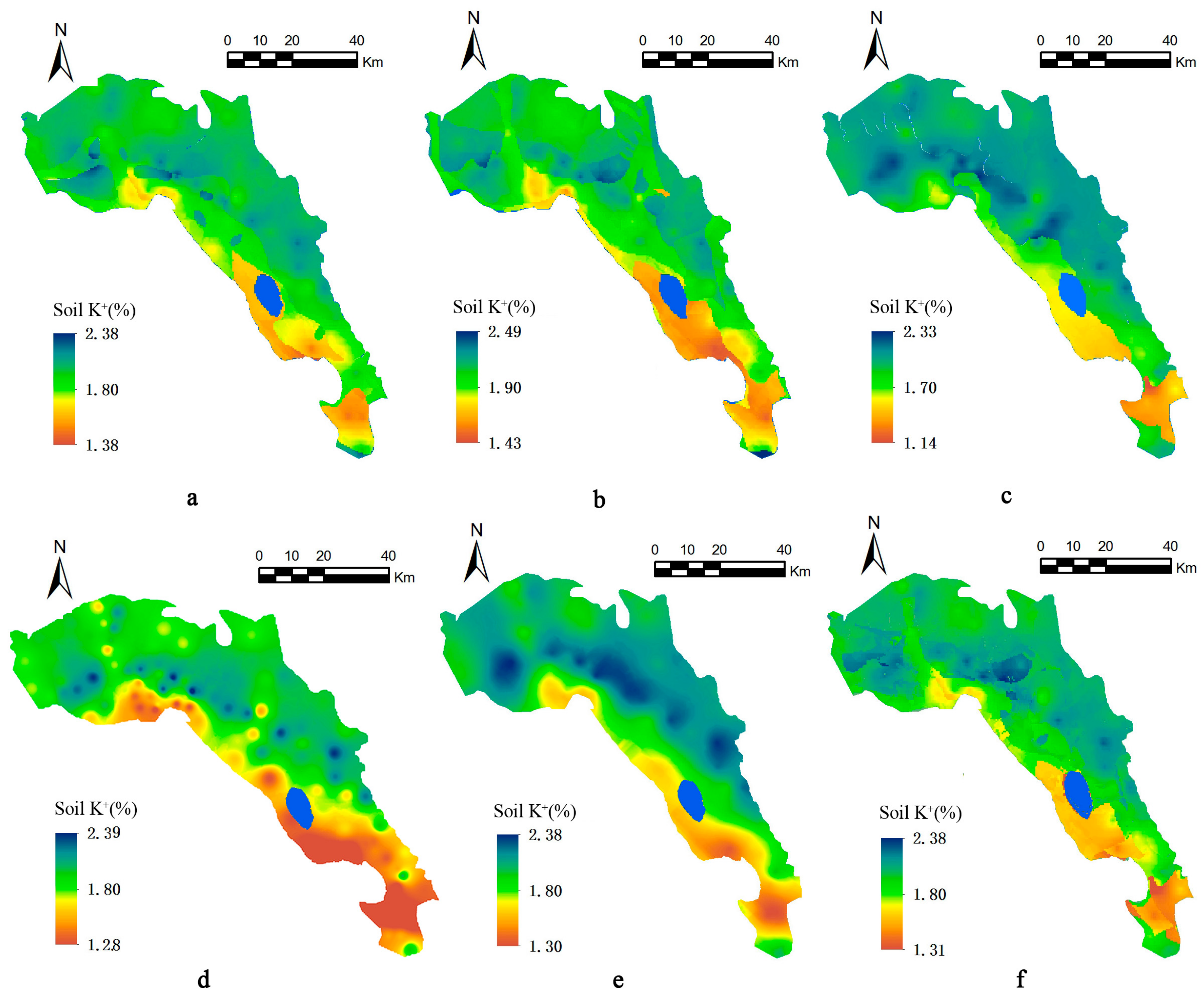
The predictive capabilities of the six interpolation methods in terms of the soil K+ maps are compared in Figure 10. The IDW interpolation gives a good representation of the overall pattern of soil K+ distribution, but the accuracy of small scale variations is low. Also, a relatively strong ‘bull’s-eye’ effect is created in areas with greater or fewer sampling points. The simulation surface of OK is smoother and its interpolation range is at an intermediate level. Owing to the smoothing effect of kriging, the range of variation in soil K+ is narrower than the true value, which is what has been found in other studies [28,29,30,31]. The OK map also shows a weak ‘bull’s-eye’ effect. The OK-Landuse, OK-Geology, and OK-Soil maps eliminate the smoothing effect of OK interpolation relatively well, and their interpolation accuracy is slightly higher. The ASM-SP method is most effective in depicting the pattern of spatial variation in soil K+ and has a moderate interpolation range (1.31–2.38), and can give more details of soil K+ distribution in different secondary variables, especially in the abrupt boundary. In contrast, soil K+ values of OK and IDW interpolation map did not have the discrete information. The method has stronger adaptability to the spatial interpolation of soil properties in areas with complex landforms, which allowed it to describe the patterns of spatial variation in soil properties in the study area more accurately.
4. Discussion
4.1. Performance of Multi-Model Integration for Reducing Predictive Error
Unlike more traditional spatial interpolation methods (e.g., IDW and OK), which use one interpolation model to train data sets, the ASM-SP method uses a series of base interpolation models and constructs error surfaces to adaptively screen and regroup the interpolation models in an optimized way. Its interpolation accuracy is usually higher than that of a single interpolation model [10]. Thus, it has great advantages for conducting interpolation with multiple models. The systematic analysis followed in this study indicates that the improved performance of the ASM-SP interpolation is mainly due to the following reasons:
- (1)
- The sample data used to predict soil properties cannot usually provide the complete information for individual interpolation models, requiring assumptions to be made about different conditions. In other words, it is difficult for a single interpolation model to accurately describe the spatial variance of soil properties across the whole study area. For instance, using sampling data for one soil property, a number of interpolation models might share similar interpolation accuracies, with no optimal interpolation. The accuracy of spatial interpolation of soil properties can be well improved by effectively combining the advantages of multiple base interpolation models.
- (2)
- The sample data used to predict soil properties often cannot accurately express patterns of spatial variation. However, the integration of multiple models is able to provide a better approximation than use of a single model. For example, the patterns of spatial variance in soil K+ in dry farmland differ greatly in areas with chernozem and clay soils. Therefore, if land use type is the only secondary variable used in the spatial interpolation of soil K+ (e.g., in OK-Landuse), it is usually impossible to achieve a relatively high prediction accuracy. An effective solution is to integrate a series of spatial interpolation methods (e.g., OK-Landuse, OK-Soil, OK-Geology, etc.) to realize simultaneous approximation.
Based on the above, it is clear that the interpolation results derived from the ASM-SP method provide a better physical explanation of the spatial variation in soil properties. Also, the simulation accuracy of ASM-SP is greatly enhanced compared with OK, OK-Landuse, OK-Soil, OK-Geology etc. Thus, ASM-SP is a more suitable method for application in areas with complex landforms.
4.2. Effectiveness of Secondary Variables for Spatial Interpolation
Different land uses, soil types, and geology all influence the spatial variation of soil properties. Previous research has also demonstrated that there is a relatively strong spatial correlation between secondary variables and the spatial variation of soil properties [14,32,33,34]. Work by [35,36] explained the correlation between the spatial variation of soil properties and secondary variables, and effectively improved the prediction accuracy of soil properties using secondary variables as secondary variables.
In this study, we compared spatial interpolation models that integrate secondary variables as the secondary variables (e.g., ASM-SP) and spatial interpolation models that do not incorporate any secondary variables (e.g., IDW and OK). The results indicated that an appropriate integration of secondary variables can effectively improve the spatial interpolation accuracy of soil properties. This supports the conclusion of Goovaerts (1999) that CoKriging interpolation combining secondary variables usually achieves a better simulation effect than OK. However, as pointed out by [24], the Cokriging interpolation result is only better than OK when the correlation between secondary variables and the sample data of soil properties is greater than 0.4. When the correlation is greater than 0.75, the simulation accuracy of spatial interpolation methods that combine secondary variables is higher than OK. Nevertheless, as shown by our previous research, the integration of secondary variables does not always effectively increase the spatial interpolation accuracy, though there is a relatively strong spatial correlation between secondary variables and the sample data of soil properties [10]. However, in general, an appropriate integration of geo-environmental factors as secondary variables is able to effectively depict soil property boundaries that abruptly change as the geo-environmental factors change.
5. Conclusions
Affected by secondary variables, the spatial distribution of soil properties is subject to problems such as spatial discontinuity and variability. It is difficult for a single global interpolation model to fully explain the spatial instability of spatial variables of soil properties, especially in areas with complex landforms. Using soil K+ as a case study, we proposed a kind of adaptive surface modeling that combines secondary variables (ASM-SP). Compared with methods such as OK and OK-Landuse, OK-Soil, and OK-Geology that also combine secondary variables, ASM-SP is able to depict the spatial variation of soil properties in areas with complex landforms more accurately, and reduce simulation errors more effectively, owing to its integration of multiple base interpolation models. In addition, since ASM-SP combines secondary variables and its simulation surface better accords with geographical laws, it provides detailed information about the spatial variation of soil properties that is more accurate and reasonable. This provides greater opportunity for physical explanation of the spatial variance characteristics of soil properties. However, ASM-SP is based on error minimization surfaces; therefore, there is a risk of over-fitting, which will be addressed in future work.
The interpolation accuracy of soil properties in areas with complex landforms has two main challenges. First, there is a non-linear relationship between the soil properties of sampling points and the secondary variables, and the fitting precision of conventional linear models is rather limited. Second, the selected interpolation model must have relatively high simulation accuracy and, preferably, provide the optimal interpolation. However, in reality, every interpolation model has advantages and disadvantages. Even though it is possible to find a global optimum interpolation model through adequate data exploration and analysis, a simple global model is unable to explain the spatial instability of soil property spatial variables. A feasible solution is to combine secondary variables to integrate multiple models, so that different combinations of interpolation models can be selected for different areas. Soil K+ is comparatively representative of soil properties that vary severely within a short horizontal distance. The ASM-SP method would also be applicable to the interpolation of other soil properties (e.g., soil P, PH, Ca, Mg, and Zn). Previously, we verified the advantages of an ensemble learning algorithm in the serial integration of multiple models [10]. In future research, we plan to comprehensively utilize the machine learning algorithm, combine secondary variables, and build and coordinate adaptive multi-model integration interpolation methods to solve over-fitting problems and to conduct high accuracy surface modeling of soil properties.
Acknowledgments
This study was supported by the National Natural Science Foundation of China (Grant No. 41601405). We are grateful to the Qinghai Environmental Monitoring Center for providing topsoil sampling approval. Thanks to the China Soil Investigation Office and the Bureau of Geological Exploration & Development of Qinghai Province for providing secondary datasets.
Author Contributions
Conceived and designed the experiments: Liu Wei; performed the experiments: Yan Da-Peng and Wang Sheng-Li; analyzed the data: Liu Wei and Zhang Hai-Rong; contributed reagents/materials/analysis tools: Wang Sheng-Li; wrote the paper: Liu Wei and Zhang Hai-Rong.
Conflicts of Interest
The authors declare no conflict of interest.
References
- Shi, W.J.; Liu, J.Y.; Du, Z.P.; Yue, T.X. High Accuracy Surface Modeling of Soil Properties Based on Geographic Information. Acta Geogr. Sin. 2011, 66, 1574–1581. [Google Scholar]
- Shi, D.; Lark, R. A New Branch of Soil Science-Pedometrics’ Its Origin and Development. Acta Pedol. Sin. 2007, 44, 919–924. [Google Scholar]
- Li, J.; Heap, A.D.; Potter, A.; Daniell, J.J. Application of Machine Learning Methods to Spatial Interpolation of Environmental Variables. Environ. Model. Softw. 2011, 26, 1647–1659. [Google Scholar] [CrossRef]
- Yue, T.X.; Wang, S.H. Adjustment Computation of Hasm: A High-Accuracy and High-Speed Method. Int. J. Geogr. Inf. Sci. 2010, 24, 1725–1743. [Google Scholar] [CrossRef]
- Wang, J.F.; Ge, Y.; Li, L.F.; Meng, B.; Wu, J.L.; Bai, Y.C. Spatiotemporal Data Analysis in Geography. Acta Geogr. Sin. 2014, 69, 1326–1345. [Google Scholar]
- Goovaerts, P. A Coherent Geostatistical Approach for Combining Choropleth Map and Field Data in the Spatial Interpolation of Soil Properties. Eur. J. Soil Sci. 2011, 62, 371–380. [Google Scholar] [CrossRef] [PubMed]
- Liu, T.L.; Juang, K.W.; Lee, D.Y. Interpolating Soil Properties Using Kriging Combined with Categorical Information of Soil Maps. Soil Sci. Soc. Am. J. 2006, 70, 1200–1209. [Google Scholar] [CrossRef]
- Gilardi, N. Machine Learning for Spatial Data Analysis. Ph.D. Thesis, University of Lausanne and Dalle Molle Institute of Perceptual Artificial Intelligence, Lausanne, Switzerland, 2002. [Google Scholar]
- Rigol, J.P.; Jarvis, C.H.; Stuart, N. Artificial Neural Networks as a Tool for Spatial Interpolation. Int. J. Geogr. Inf. Sci. 2001, 15, 323–343. [Google Scholar] [CrossRef]
- Liu, W.; Du, P.J.; Zhao, Z.W.; Zhang, L.P. An Adaptive Weighting Algorithm for Interpolating the Soil Potassium Content. Sci. Rep. 2016, 6, 23889. [Google Scholar] [CrossRef] [PubMed]
- Bashir, B.; Fouli, H. Studying the Spatial Distribution of Maximum Monthly Rainfall in Selected Regions of Saudi Arabia Using Geographic Information Systems. Arab. J. Geosci. 2015, 8, 1–15. [Google Scholar] [CrossRef]
- Borůvka, L.; Mládková, L.; Penížek, V.; Drábek, O.; Vašát, R. Forest Soil Acidification Assessment Using Principal Component Analysis and Geostatistics. Geoderma 2007, 140, 374–382. [Google Scholar] [CrossRef]
- Florinsky, I.; Eilers, R.G.; Manning, G.; Fuller, L. Prediction of Soil Properties by Digital Terrain Modelling. Environ. Model. Softw. 2002, 17, 295–311. [Google Scholar] [CrossRef]
- Kuriakose, S.L.; Devkota, S.; Rossiter, D.; Jetten, V. Prediction of Soil Depth Using Environmental Variables in An Anthropogenic Landscape, a Case Study in the Western Ghats of Kerala, India. Catena 2009, 79, 27–38. [Google Scholar] [CrossRef]
- Li, B.; Zhang, Y.; Shi, X.; Zhang, K.; Zhang, J. Spatial Interpolation Method Based on Integrated Rbf Neural Networks for Estimating Heavy Metals in Soil of a Mountain Region. J. Southeast Univ. 2015, 31, 38–45. [Google Scholar]
- Minasny, B.; Mcbratney, A.B. Spatial Prediction of Soil Properties Using Eblup with the Matérn Covariance Function. Geoderma 2007, 140, 324–336. [Google Scholar] [CrossRef]
- Montealegre, A.; Lamelas, M.; Riva, J. Interpolation Routines Assessment in Als-Derived Digital Elevation Models for Forestry Applications. Remote Sens. 2015, 7, 8631–8654. [Google Scholar] [CrossRef]
- Yang, S.H.; Zhang, H.T.; Guo, L.; Ren, Y. Spatial Interpolation of Soil Organic Matter Using Regression Kriging and Geographically Weighted Regression Kriging. Chin. J. Appl. Ecol. 2015, 26, 1649–1656. [Google Scholar]
- Liu, W.; Du, P.J.; Wang, D.C. Ensemble Learning for Spatial Interpolation of Soil Potassium Content Based on Environmental Information. PLoS ONE 2015, 10, e0124383. [Google Scholar] [CrossRef] [PubMed]
- Zhang, H.; Lu, L.; Liu, Y.; Liu, W. Spatial Sampling Strategies for the Effect of Interpolation Accuracy. ISPRS Int. J. Geo-Inf. 2015, 4, 2742–2768. [Google Scholar] [CrossRef]
- Sparks, D.L.; Page, A.L.; Helmke, P.A.; Loeppert, R.H.; Soltanpour, P.N.; Tabatabai, M.A.; Johnston, C.T.; Sumner, M.E. Methods of Soil Analysis. Part 3—Chemical Methods; Soil Science Society of America: Fitchburg, WI, USA, 2009. [Google Scholar]
- Burrough, P.A. Principles of Geographical Information Systems for Land Resources Assessment. Geocarto Int. 1987, 1, 102. [Google Scholar] [CrossRef]
- Mosammam, A. Geostatistics: Modeling Spatial Uncertainty. J. Appl. Stat. 2013, 40, 923. [Google Scholar] [CrossRef]
- Asli, M.; Marcotte, D. Comparison of Approaches to Spatial Estimation in a Bivariate Context. Math. Geol. 1995, 27, 641–658. [Google Scholar] [CrossRef]
- Odeh, I.O.; Mcbratney, A.; Chittleborough, D. Further Results on Prediction of Soil Properties From Terrain Attributes: Heterotopic Cokriging and Regression-Kriging. Geoderma 1995, 67, 215–226. [Google Scholar] [CrossRef]
- Hengl, T.; Heuvelink, G.; Stein, A. A Generic Framework for Spatial Prediction of Soil Variables Based on Regression-Kriging. Geoderma 2004, 120, 75–93. [Google Scholar] [CrossRef]
- Cambardella, C.A.; Karlen, D.L. Spatial Analysis of Soil Fertility Parameters. Precis. Agric. 1999, 1, 5–14. [Google Scholar] [CrossRef]
- Long, J.; Zhang, L.M.; Zhou, B.Q.; Mao, Y.L.; Qiu, L.X.; Xing, S.H. Spatial Interpolatin of Soil Organic Matter in Farmlands in Areas Complex in Landform. Acta Pedol. Sin. 2014, 51, 81–93. [Google Scholar]
- Penížek, V.; Borůvka, L. Soil Depth Prediction Supported by Primary Terrain Attributes: A Comparison of Methods. Plant Soil Environ. 2006, 52, 424–430. [Google Scholar]
- Triantafilis, J.; Odeh, I.; Mcbratney, A. Five geostatistical models to predict soil salinity from Electromagnetic induction data across irrigated cotton. Soil Sci. Soc. Am. J. 2001, 65, 869–878. [Google Scholar] [CrossRef]
- Zhao, Y.F.; Sun, Z.Y.; Chen, J. Analysis and Comparison in Arithmetic for Kriging Interpolation and Sequential Gaussian Conditional Simulation. J. Geo-Inf. Sci. 2010, 6, 767–776. [Google Scholar] [CrossRef]
- Li, Q.Q.; Wang, C.Q.; Yue, T.X.; Li, B.; Zhang, X.; Gao, X.S.; Zhang, Y. Prediction of Distribution of Soil Organic Matter Based on Qualitative and Antitative Auxiliary Variables: A Case Study in Santai County in Sichuan Province. Progress Geogr. 2014, 33, 259–269. [Google Scholar]
- Qiu, L.F.; Yang, C.; Lin, F.F.; Yang, N.; Zhen, X.H. Spatial Pattern of Soil Fertility in Bashan Tea Garden: A Prediction Based on Environmental Auxiliary Variables. Chin. J. Appl. Ecol. 2010, 21, 3099–3104. [Google Scholar]
- Wen, W.; Zhou, B.T.; Wang, Y.F.; Huang, Y. Soil Organic Carbon Interpolation Based on Auxiliary Environmental Covariates: A Case Study At Small Watershed Scale in Loess Hilly Region. Acta Ecol. Sin. 2013, 33, 6389–6397. [Google Scholar] [CrossRef]
- Hu, K.; Li, H.; Li, B.; Huang, Y. Spatial and Temporal Patterns of Soil Organic Matter in the Urban–Rural Transition Zone of Beijing. Geoderma 2007, 141, 302–310. [Google Scholar] [CrossRef]
- Shi, W.; Liu, J.; Du, Z.; Stein, A.; Yue, T. Surface Modelling of Soil Properties Based on Land Use Information. Geoderma 2011, 162, 347–357. [Google Scholar] [CrossRef]
Figure 1.
Location of the study area, showing sample sites (circles) and elevation (shading).

Figure 2.
Characteristics of the study area: (a) soil types, from the 1: 1,000,000 soil map of the China Soil Investigation Office; (b) geology types, from the 1:500,000 geologic map of the Bureau of Geological Exploration and Development of Qinghai Province; (c) land use types; and (d) grassland types.

Figure 3.
Adaptive partitioning process (a) and clustering (b).

Figure 4.
Semi-variograms of soil K+ residuals for: (a) OK-Soil; (b) OK-Geology; (c) OK-Landuse; and (d) OK (original values).
Figure 4.
Semi-variograms of soil K+ residuals for: (a) OK-Soil; (b) OK-Geology; (c) OK-Landuse; and (d) OK (original values).

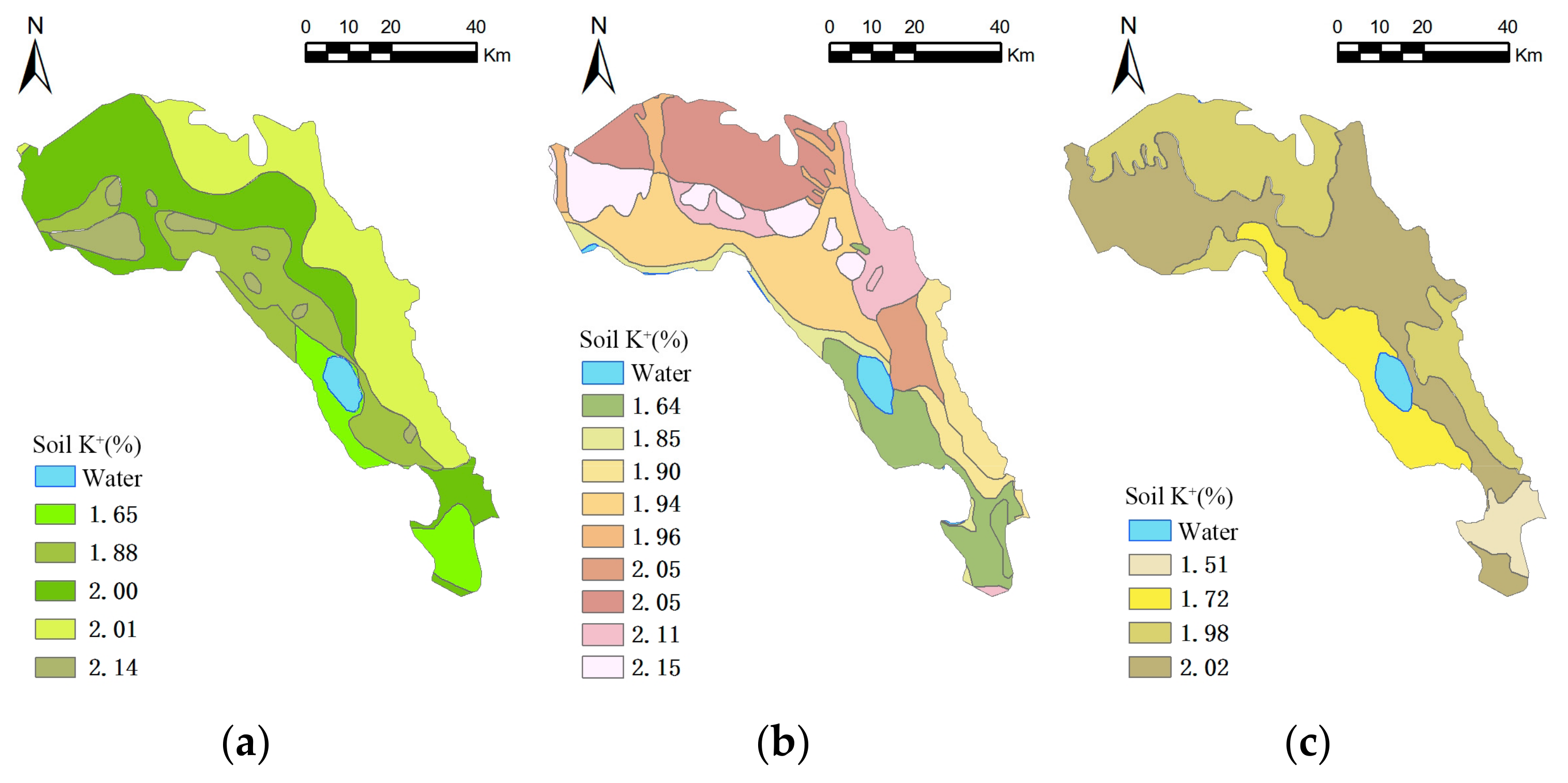
Figure 5.
Mean surface m(Emn) of soil K+ for different secondary variables: (a) land use; (b) geology; (c) soil type.
Figure 5.
Mean surface m(Emn) of soil K+ for different secondary variables: (a) land use; (b) geology; (c) soil type.

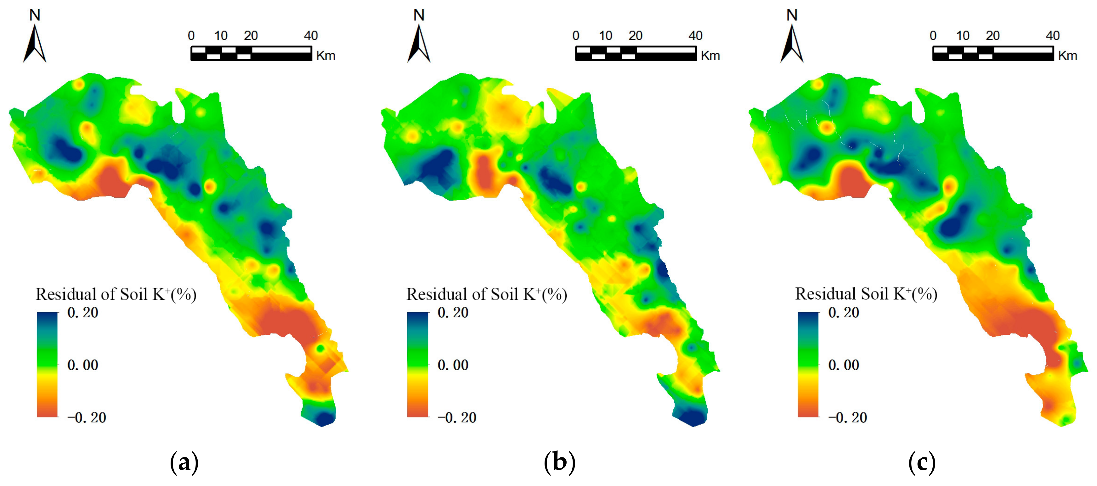
Figure 6.
Residual surfaces r(xmn,ymn) of soil K+ for different secondary variables: (a) land use; (b) geology; (c) soil type.
Figure 6.
Residual surfaces r(xmn,ymn) of soil K+ for different secondary variables: (a) land use; (b) geology; (c) soil type.

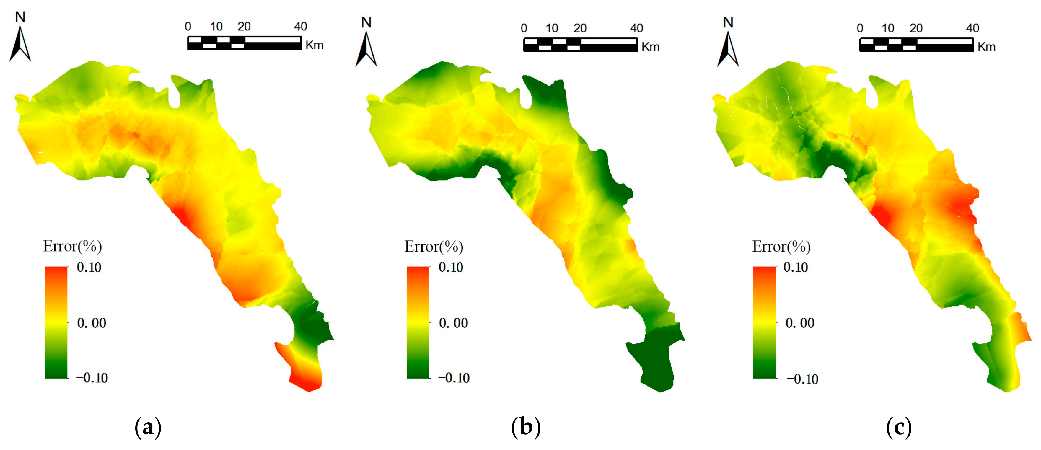
Figure 7.
Error surfaces of base interpolation models: (a) land use; (b) geology; (c) soil type.

Figure 8.
The raster cell optimization process (‘a’ and ‘b’ are different models of raster interpolation, ‘c’ and ‘d’ are the interpolation error, ‘e’ is the optimal raster cell mosaic result).
Figure 8.
The raster cell optimization process (‘a’ and ‘b’ are different models of raster interpolation, ‘c’ and ‘d’ are the interpolation error, ‘e’ is the optimal raster cell mosaic result).

Figure 9.
Regional distribution of optimized base interpolation models.

Figure 10.
Comparison of soil K+ maps constructed using different interpolation methods: (a) OK-Landuse, where OK is ordinary kriging; (b) OK-Geology; (c) OK-Soil; (d) inverse distance weighting (IDW); (e) OK; and (f) ASM-SP.
Figure 10.
Comparison of soil K+ maps constructed using different interpolation methods: (a) OK-Landuse, where OK is ordinary kriging; (b) OK-Geology; (c) OK-Soil; (d) inverse distance weighting (IDW); (e) OK; and (f) ASM-SP.


Table 1.
Descriptive statistical characteristics of soil K+ content in different secondary variables.
Table 1.
Descriptive statistical characteristics of soil K+ content in different secondary variables.
| Secondary Variable | Subtype | Number | Mean | Standard Error | Area/km2 | Area Proportion/% |
|---|---|---|---|---|---|---|
| Soil | Alpine meadow soil | 32 | 1.98 | 0.14 | 420.47 | 20.81 |
| Chestnut soil | 54 | 2.01 | 0.18 | 1360.14 | 67.31 | |
| Flow sandy soil | 10 | 1.72 | 0.12 | 144.76 | 7.16 | |
| Meadow marsh soil | 6 | 1.84 | 0.03 | 31.9 | 1.58 | |
| Semi-fixed sandy soil | 8 | 1.50 | 0.07 | 63.4 | 3.14 | |
| Geology | Alluvial terrace | 8 | 2.04 | 0.14 | 71.25 | 3.53 |
| Denudate high terrace | 10 | 2.15 | 0.07 | 266.73 | 13.22 | |
| Diluvial plain | 13 | 2.10 | 0.13 | 515.24 | 25.53 | |
| Hilly | 3 | 2.14 | 0.05 | 3.76 | 0.19 | |
| Lacustrine plain | 20 | 1.94 | 0.17 | 333.33 | 16.52 | |
| Lake beach | 5 | 1.84 | 0.09 | 143.99 | 7.14 | |
| Large rolling alpine | 10 | 1.89 | 0.12 | 132.64 | 6.57 | |
| Middle rolling alpine | 4 | 1.91 | 0.10 | 5.63 | 0.28 | |
| Sand dune | 14 | 1.63 | 0.14 | 193.15 | 9.57 | |
| Small rolling alpine | 14 | 2.05 | 0.12 | 287.08 | 14.23 | |
| Valley plain | 9 | 1.96 | 0.08 | 65.22 | 3.23 | |
| Land use | Cropland | 10 | 2.14 | 0.08 | 77.16 | 3.83 |
| Grassland | 41 | 1.99 | 0.13 | 1172.65 | 58.17 | |
| Meadowland | 25 | 2.02 | 0.12 | 417.44 | 20.71 | |
| Potential arable land | 16 | 1.88 | 0.14 | 229.32 | 11.38 | |
| Scrubland | 0 | 1.91 | 0.22 | 1.18 | 0.05 | |
| Swamp meadowland | 5 | 1.84 | 0.04 | 32.09 | 1.59 | |
| Unused land | 13 | 1.64 | 0.09 | 86.43 | 4.29 | |
| Grassland | Achnatherum splendens | 37 | 1.93 | 0.17 | 719.58 | 35.59 |
| Artemisaarenariadc | 2 | 1.49 | 0.07 | 31.83 | 1.57 | |
| Blysmus sinocompressus | 5 | 1.93 | 0.14 | 30.00 | 1.48 | |
| Bush cinqefoil | 18 | 2.06 | 0.14 | 517.19 | 25.58 | |
| Coarse beak carex | 2 | 1.86 | 0.04 | 20.10 | 0.99 | |
| Elymus nutans | 3 | 1.73 | 0.08 | 18.49 | 0.91 | |
| Ephedra | 1 | 1.50 | 0 | 2.49 | 0.12 | |
| Gravel | 4 | 1.68 | 0.10 | 135.38 | 6.70 | |
| Iris ensata thunb | 1 | 1.96 | 0 | 34.47 | 1.70 | |
| Leymus | 6 | 1.94 | 0.27 | 28.95 | 1.43 | |
| Kobresia humilis | 4 | 2.02 | 0.08 | 28.30 | 1.40 | |
| Koeleria tibetica | 4 | 1.80 | 0.10 | 24.45 | 1.21 | |
| Kobresia capillifolia | 7 | 2.05 | 0.08 | 157.90 | 7.81 | |
| Kobresia myosuroides | 3 | 2.16 | 0.06 | 82.99 | 4.11 | |
| Salix oritrepha | 2 | 2.02 | 0.05 | 16.33 | 0.81 | |
| Serpent grass | 2 | 1.94 | 0.08 | 4.29 | 0.21 | |
| Stipa krylovii | 3 | 1.82 | 0.05 | 51.77 | 2.56 | |
| Stipa purpurea | 5 | 2.14 | 0.07 | 111.51 | 5.52 | |
| Water bai zhi | 1 | 2.08 | 0 | 5.64 | 0.28 |
Table 2.
Semi-variogram models.
| Parameter | Residue of OK_Landuse | Residue of OK_Soil | Residue of OK_Geology | OK |
|---|---|---|---|---|
| Model | K-Bessel | K-Bessel | Exponential | Exponential |
| Range/10 km | 1.1984 | 1.2169 | 1.1984 | 2.5058 |
| Nugget (N) | 0.0204 | 0.03124 | 0.1866 | 0.2483 |
| Sill (S) | 0.4842 | 0.5043 | 0.4783 | 0.6012 |
| N/S | 0.0421 | 0.0619 | 0.3901 | 0.4130 |
Table 3.
ANOVA analysis for testing the significance of secondary variables on soil K+ variance.
| Geo-Factors | Soil Property | Sources of Variance | Degree of Freedom | Sum of Variance | Mean Variance | F Value | p Value |
|---|---|---|---|---|---|---|---|
| Geology type | Soil K+ | In-group | 9 | 1.033 | 0.115 | 2.856 | 0.005 |
| Between groups | 101 | 4.060 | 0.04 | ||||
| Total | 110 | 5.093 | |||||
| Soil type | Soil K+ | In-group | 4 | 0.722 | 0.181 | 4.378 | 0.003 |
| Between groups | 106 | 4.371 | 0.041 | ||||
| Total | 110 | 5.093 | |||||
| Land use type | Soil K+ | In-group | 4 | 0.462 | 0.116 | 2.645 | 0.008 |
| Between groups | 106 | 4.631 | 0.044 | ||||
| Total | 110 | 5.093 | |||||
| Grassland type | Soil K+ | In-group | 16 | 0.934 | 0.058 | 1.319 | 0.202 |
| Between groups | 94 | 4.159 | 0.044 | ||||
| Total | 110 | 5.093 |
Table 4.
Comparison of the accuracy of OK, OK-Landuse, OK-Geology, OK-Soil, inverse distance weighting (IDW), and ASM-SP interpolation.
Table 4.
Comparison of the accuracy of OK, OK-Landuse, OK-Geology, OK-Soil, inverse distance weighting (IDW), and ASM-SP interpolation.
| Evaluation Index | OK-Landuse | OK-Geology | OK-Soil | IDW | OK | ASM-SP |
|---|---|---|---|---|---|---|
| ME | 0.0030 | −0.0037 | 0.0024 | 0.0072 | 0.0093 | 0.0017 |
| MAE | 0.0294 | 0.0301 | 0.0236 | 0.0362 | 0.0314 | 0.0072 |
| RMSE | 0.0742 | 0.0672 | 0.0815 | 0.1637 | 0.1067 | 0.0586 |
| MRE | 95.91% | 96.57% | 95.87% | 96.04% | 95.34% | 89.69% |
| AC | 0.9047 | 0.9186 | 0.9242 | 0.8756 | 0.8976 | 0.9903 |
© 2017 by the authors. Licensee MDPI, Basel, Switzerland. This article is an open access article distributed under the terms and conditions of the Creative Commons Attribution (CC BY) license (http://creativecommons.org/licenses/by/4.0/).
Share and Cite
MDPI and ACS Style
Liu, W.; Zhang, H.-R.; Yan, D.-P.; Wang, S.-L. Adaptive Surface Modeling of Soil Properties in Complex Landforms. ISPRS Int. J. Geo-Inf. 2017, 6, 178. https://doi.org/10.3390/ijgi6060178
AMA Style
Liu W, Zhang H-R, Yan D-P, Wang S-L. Adaptive Surface Modeling of Soil Properties in Complex Landforms. ISPRS International Journal of Geo-Information. 2017; 6(6):178. https://doi.org/10.3390/ijgi6060178
Chicago/Turabian StyleLiu, Wei, Hai-Rong Zhang, Da-Peng Yan, and Sheng-Li Wang. 2017. "Adaptive Surface Modeling of Soil Properties in Complex Landforms" ISPRS International Journal of Geo-Information 6, no. 6: 178. https://doi.org/10.3390/ijgi6060178
Note that from the first issue of 2016, this journal uses article numbers instead of page numbers. See further details here.