Proposed Consecutive Uncertainty Analysis Procedure of the Greenhouse Gas Emission Model Output for Products

Abstract

The study objective was to develop a method for an uncertainty analysis of the greenhouse gas (GHG) emission model output based on consecutive use of an analytical and a stochastic approach. The contribution to variance (CTV) analysis followed by the data quality analysis are the main feature of the procedure. When a set of data points of a certain input variable has a high CTV, but its data quality indicator (DQI) is good, then there is no need to iterate data collection of this input variable. This is because the DQI of this data set indicates that there is no room for the reduction of its variance, and the high variance must be its inherent attribute. Through the CTV analysis and data quality analysis, the identified input variables were selected as the input variables for the data from the iteration of data collection. The statistical parameters of the GHG emissions of the model were calculated using the Monte Carlo simulation (MCS). In the case study of a cattle dairy farm, the relative reduction in the CV value was 47.6%. In this study, a procedure was developed for the selection of the input variables for iteration of data collection to reduce their variance and subsequently reduce the uncertainty in the model output. The dairy cow case study showed that the uncertainty in the model output was decreased by the iteration of data collection, indicating that CTV analysis can be used to identify the input variables, contributing considerably to the uncertainty in the model output.

1. Introduction

It is an international consensus that human production and consumption activities cause climate change [1]. In recent years, life cycle assessment (LCA) studies have been extended to food production and cooking appliances [2,3]. This is a phenomenon that confirms that interest in the environmental impacts that occur throughout human life in the LCA field has increased.

According to previous studies, the contribution of greenhouse gas (GHG) emissions in the dairy sector is estimated to be 3–5% of the global GHG missions. In Korea, various efforts are being made to reduce GHG emissions in the dairy sector and there is a growing demand for accuracy [4,5,6,7].

In Europe, an effort is being made to manage and control GHG emissions not only from the industrial products sectors but also from the dairy industry sector through the product environmental footprint (PEF). This includes the development of the quantification method of GHG emissions from the dairy sector [8,9]. This effort can be envisaged as a prelude to the certification of carbon emissions in Europe. Any carbon certification or trading requires that the credibility of the GHG emission results, such as the quantification in the uncertainty of the GHG emission resulting from the industry sectors or product, is necessary and must be ensured [10].

Uncertainty analysis is the analysis of the mathematical model output by quantifying the amount of deviation of the calculated model output from its mean. The uncertainty analysis result is often expressed as a confidence interval at a given confidence level. Quite often, the model inputs suffer from observation and measurement errors. This causes a limit on the confidence in the model output [11].

In order to gain confidence in the model output, the mathematical model should include the following two evaluation steps: a quantification of the uncertainty in the model output (uncertainty analysis) and an evaluation of how much each input variable contributes to the uncertainty of the model output (sensitivity analysis) [12].

Normally, there are many input variables in the mathematical model. Therefore, an efficient scheme needs to be developed for identifying input variables that considerably contribute to the uncertainty of the model output. Global sensitivity analysis is an effective tool for identifying input variables contributing to the model output uncertainty [12,13,14,15,16].

Uncertainty can be reduced through the process of iteration of data collection [17]. Therefore, those identified input variables will become targets for further scrutiny, including iteration of data collection.

The global sensitivity method used in this study was a modification of the variance-based method [18,19,20,21]. The variance-based method uses probabilistic approaches, which quantify the input and output uncertainty using their probability distributions. It also decomposes the output variance into parts attributable to input variables [12].

The objective of this study was two-fold: (i) to perform a global sensitivity analysis for identifying the input variables that contribute considerably to the uncertainty of the model output and (ii) to quantify the uncertainty reduction of the model output when the data from iteration of data collection of the identified input variables are used instead of the original data. The actual process and activity data collected from a dairy cow farm in Korea [22] were used to evaluate the applicability of the proposed method.

2. Materials and Methods

The uncertainty of each variable can affect the uncertainty of the result, and the variance of each variable can be used as an indicator to represent the uncertainty of the variable [23]. The process of reducing variance helps to correctly estimate the mean of the overall results [23]. This means that it is important to select significant variables in order to effectively reduce the uncertainty of the results.

In this study, we used the error propagation method in lieu of the probabilistic approach for identifying key input parameters which affect the uncertainty of the carbon footprint result. This was to avoid an excessive computing time in selecting the key input parameters. The contributions of input parameters to the uncertainty of the result were evaluated by the contributions of the input parameters to the variance of the results. This was the concept of the contribution to variance (CTV).

The global sensitivity analysis approach, termed analytical approach in this study had two elements which were the variance calculation of the model output using the error propagation equation and the identification of the significant input variables using the CTV analysis. The sensitivity analysis results led us to focus on the identified input variables where their errors were reduced through iteration of data collection and we simplified the mathematical model by removing the iteration of data collection process for insignificant input variables as in studies dealing with a single environmental issue, such as carbon footprint.

The reason for coining the term “analytical approach” here was that no stochastic simulations were included in the variance calculation step for the sensitivity analysis. If time and resources are not constraints, then one can use the stochastic approach from the beginning without going through the error propagation equation step and obtain the uncertainty of the model output based on the variance-based approach. However, the iteration of data collection process expenses were a major hurdle in this case.

After the analytical approach, the model underwent stochastic simulation to calculate the uncertainty of the model output. This required estimating the probability density function (PDF) of the input variables, its data ranges, and generating the model output using the Monte Carlo simulation method. From the model output values, the interval estimate of the model output was calculated at a 95% confidence level.

In addition to the sensitivity analysis, we also included a data quality indicator (DQI) concept to reduce the number of input variables for iteration of data collection. Temporal, geographical, and technological characteristics of the data influenced the mean and variance of each variable, and these characteristics were used as the DQI evaluation factors [23]. High data quality meant that the accuracy and precision of the collected data for the variable was less likely to be reduced. We assumed the CTV analysis identified input variables that contributed considerably to the model output. If the data of the input variable had inherently high variance (a representative example of an input variable with inherently high variance was ingredient feeds and roughage feeds that were applied alternatively according to price fluctuation, such as soy bean, alfalfa hay, grass hay, etc.), then, there was no room for reducing the sample variance of that input variable, even if we collected more data points with higher precision. Therefore, the purpose of introducing the DQI concept was to add one more filter before commencing iteration of data collection.

For assessing the environmental impact of the GHG emissions from a dairy cow farm system, a mathematical model was formulated. The model was defined by equations, input variables, and relevant coefficients.

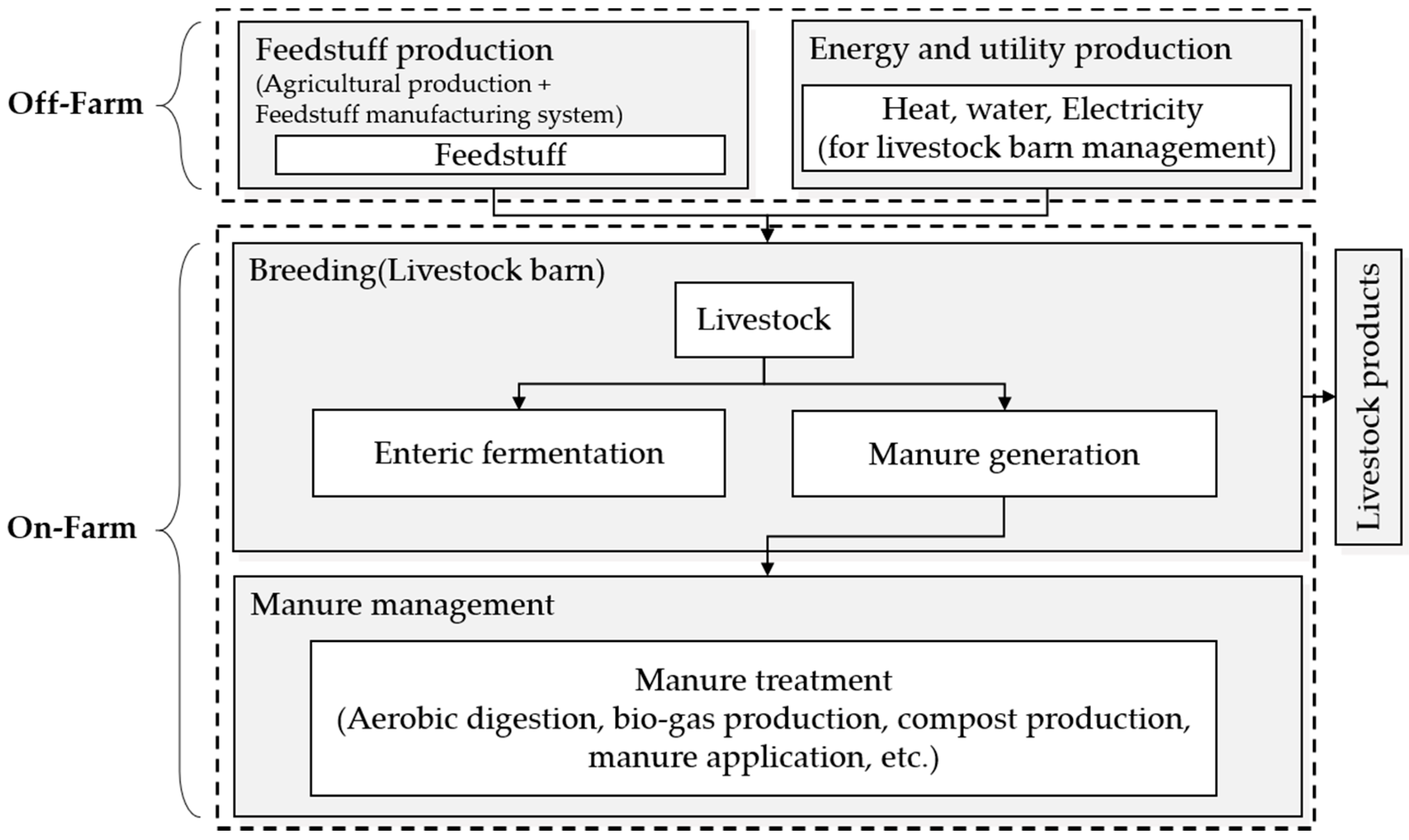
This study addressed only uncertainty in GHG emission from on-farm data. Figure 1 shows the concept of on-farm and off-farm processes. In this study, the upstream processes in off-farm, such as feedstuff cultivation, energy, and utility production processes were excluded from active data collection. This was because the research conditions were incomplete, so the activity data up to the data on the cultivation of the feedstuff could not be used. The GHG emissions for upstream processes were calculated using the pre-established LCI database, and the uncertainty of the LCI database was not considered in this study. Functional unit was set to 1kg of Fat-Protein Corrected Milk (FPCM).

The greenhouse gas (GHG) emission model, in general, was expressed as the linear function as shown in Equation (1):

$$\mathrm{z}={{\displaystyle \sum }}^{}{\mathrm{a}}_{\mathrm{i}}·{\mathrm{X}}_{\mathrm{i}},$$

(1)

where:

• $\mathrm{z}$ = GHG model output, g CO₂–eq/fu,
• a_i = GHG emission factor, g CO₂–eq/g of the ith substance,
• X_i = mass (energy) of the ith substance, g(J),
• fu = functional unit (1 kg of FPCM).

The data of the input variables, X_i, were collected and then plugged into Equation (1) to calculate the model output, z. The GHG emission factor, ai, comes from the LCI database [24]. Variance, mean, and coefficient of variation (CV) of z were calculated to assess the uncertainty of the model output. It was often desirable to use the contribution to variance (CTV) to judge the degree of dispersion of the data of a random variable and the output of a model [11,25].

The data of the input variables, such as data of the processes and activities (i.e., the amount of feed intake, energy use, number of heads, etc.) were subject to a variety of errors, including completeness, representativeness, and boundaries, such as temporal, geographical, and technological. In other words, the data quality of the input variables is questionable [26]. Without considering the data quality of the input data, the GHG model output would suffer from the errors of the input variables.

However, there were instances where an input variable had an inherently high variance in nature, such as soy bean, alfalfa hay, grass hay, etc. In this case, iteration of data collection did not reduce the variance of the model output. Therefore, such input variables were not subjected to iteration of data collection.

Once particular input variables exhibited high CTV with poor data quality, those particular input variables underwent iteration of data collection. The new mean, variance, and CV of the model output were then calculated using the data from the iteration of data collection. The entire procedure was repeated until all the conditions specified in Figure 2 were met.

This paper adopted the global sensitivity analysis method for identifying input variables that influence the model output. The expression for the variance of the model output, $\mathrm{z}$, could be obtained using the Taylor Series 1st order approximation and definition of the error propagation equation [14,27,28,29]. The resulting expression was termed as the error propagation equation and is shown in Equation (2):

$${\mathsf{\sigma }}_{\mathrm{z}}^2={{\displaystyle \sum }}^{}{\mathsf{\sigma }}_{{\mathrm{X}}_{\mathrm{i}}}^2·{\left(\partial \mathrm{z}/\partial {\mathrm{X}}_{\mathrm{i}}\right)}^2+2·{{\displaystyle \sum }}^{}\left(\frac{\partial \mathrm{z}}{\partial {\mathrm{X}}_{\mathrm{i}}}\right)\left(\frac{\partial \mathrm{z}}{\partial {\mathrm{X}}_{\mathrm{i}+1}}\right){\sigma }_{{\mathrm{X}}_{\mathrm{i}}{\mathrm{X}}_{\mathrm{i}+1}}^2,$$

(2)

where:

• ${\mathsf{\sigma }}_{\mathrm{z}}^2$ = the variance of the model output, z,
• ${\mathsf{\sigma }}_{{\mathrm{X}}_{\mathrm{i}}}^2$ = the variance of the input variable, X_i,
• $\partial \mathrm{z}/\partial {\mathrm{X}}_{\mathrm{i}}$ = the sensitivity coefficient of the input variable, X_i,
• ${\sigma }_{{\mathrm{X}}_{\mathrm{i}}{\mathrm{X}}_{\mathrm{i}+1}}^2$ = covariance of the input variables, X_i, X_i+1.

Equation (2) was a generic equation for the quantification of the variance of the model output as a function of the variances of the input variables and their sensitivity coefficients. Furthermore, GHG emission was chosen as the model output to apply the identification methodology proposed in this study. In this sense, the identification methodology could be applied to any other impact categories.

In most LCI databases and LCIA studies, covariance can be assumed to be negligible [30]. Therefore, we used Equation (2) by setting the covariance term to zero. Equation (2) shows that the variances of the input variables weighted by the square of their partial derivatives determine ${\mathsf{\sigma }}_{\mathrm{z}}^2$. The variance of the input variables caused the uncertainty of the model output. The error propagation equation indicates that the uncertainty of each input variable propagated uncertainty through the model and resulted in model output uncertainty.

Equation (2) also shows that the value of ${\mathsf{\sigma }}_{{\mathrm{X}}_{\mathrm{i}}}^2·{\left(\partial \mathrm{z}/\partial {\mathrm{X}}_{\mathrm{i}}\right)}^2$ represents the degree of contribution of the input variable ${\mathrm{X}}_{\mathrm{i}}$ to the variance of the model output, i.e., ${\mathsf{\sigma }}_{\mathrm{z}}^2$, and the CTV of ${\mathrm{X}}_{\mathrm{i}}$ to ${\mathsf{\sigma }}_{\mathrm{z}}^2$ as expressed in Equation (3) should be used as the criterion for identifying the significant input variable [14]:

$$\mathrm{CTV} \mathrm{of} {\mathrm{X}}_{\mathrm{i}} = \left\{{\mathsf{\sigma }}_{{\mathrm{X}}_{\mathrm{i}}}^2·{\left(\partial \mathrm{z}/\partial {\mathrm{X}}_{\mathrm{i}}\right)}^2\right\}/{\mathsf{\sigma }}_{\mathrm{z}}^2.$$

(3)

A variable ${\mathrm{X}}_{\mathrm{i}}$ identified with high CTV did not automatically indicate that it became the target for iteration of data collection. One needed to investigate the data quality of the identified input variable.

When a set of data points of a certain input variable had a high ${\mathsf{\sigma }}_{{\mathrm{X}}_{\mathrm{i}}}^2·{\left(\partial \mathrm{z}/\partial {\mathrm{X}}_{\mathrm{i}}\right)}^2,$ but its data quality indicator (DQI) was good, then there was no need to iterate data collection of this input variable. This was because the DQI of this dataset indicated that there was no room for the reduction of its variance, and the high variance must be its inherent attribute.

It should be pointed out that no direct relationship existed between the DQI and variance of an input variable. However, in the case of an input variable with a poor DQI, there was a possibility of having high variability of data because of the following data quality areas: time-related coverage, geographical related coverage, technology coverage, precision, completeness, representativeness, consistency, and sources of data. If this was the case, the variance of the input variable was reduced through iteration of data collection. As a result, its DQI could be improved. As such, choosing the input variable with a poor DQI as well as high CTV for iteration of data collection would be an effective means of reducing the variance of the model output.

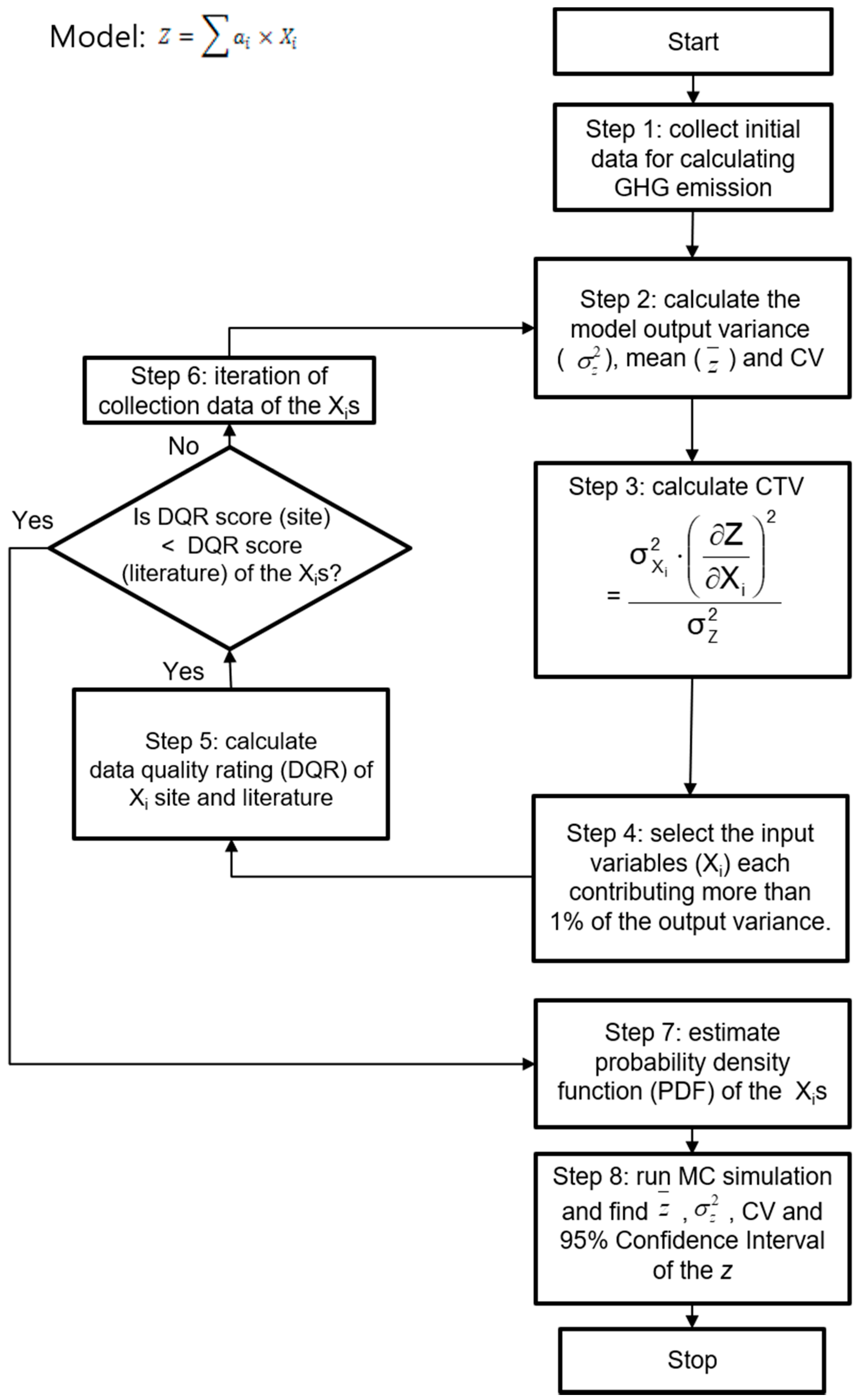
Figure 2 shows the step-by-step procedure for identifying the input variables that contributed considerably to the uncertainty of the model output together with the uncertainty quantification procedure of the model output.

The description of the steps in Figure 2 together with rationale for each step are shown below.

• Step 1 collect initial data for calculating the GHG emission.

Before any data collection activity began, a target farm had to be chosen based on the random sampling technique. Here, we used the stratum sampling method [20]. The stratum used in this study was a dairy cow farm that fed its cow using the standard feed mixture. Since one of the objectives of the study was to validate the identification methodology for reducing the uncertainty of the model output, only one typical Korean dairy farm was chosen.

There were two principles in the data collection of the input variables adopted in this study. The first principle was that onsite data would be collected as much as possible. The second principle was that the data collection period would span at least one year to reflect the seasonal variations of the dairy cow farm. Data sources in this study included the invoice of the feedstuff, materials, and energy, and the growth record of the number of heads on the farm.

Table 1. Statistics of the input variables of the target dairy farm (normalized value).

Category	Input Variable	Maximum	Minimum	Mean	Standard Deviation	CV (%)
Mixed feed	Feed for dry cows (kg/kg FPCM)	6.30 × 10−2	3.85 × 10−3	3.54 × 10−2	1.70 × 10−2	48.02
	Feed for lactating cows (kg/kg FPCM)	4.92 × 10−1	1.94 × 10−1	3.26 × 10−1	1.08 × 10−1	33.13
Roughage feed	Alfalfa (kg/kg FPCM)	8.73 × 10−2	2.33 × 10−2	6.43 × 10−2	1.80 × 10−2	27.99
	Straw (kg/kg FPCM)	1.48 × 10−1	1.60 × 10−2	6.40 × 10−2	3.26 × 10−2	50.94
	Oat (kg/kg FPCM)	1.51 × 10−1	1.64 × 10−2	6.36 × 10−2	4.99 × 10−2	78.46
	Maize silage (kg/kg FPCM)	6.75 × 10−1	9.90 × 10−2	3.32 × 10−1	1.67 × 10−1	50.30
Ingredient feed	Rapeseed mill (kg/kg FPCM)	7.18 × 10−2	2.29 × 10−2	5.35 × 10−2	1.46 × 10−2	27.29
	Bagasse (kg/kg FPCM)	1.36 × 10−1	1.01 × 10−2	4.98 × 10−2	3.41 × 10−2	68.47
	Soybean (kg/kg FPCM)	1.12 × 10−2	9.00 × 10−2	4.04 × 10−2	1.93 × 10−2	47.77
Energy	Electricity (kWh/kg FPCM)	4.73 × 10−1	7.14 × 10−2	3.02 × 10−1	1.29 × 10−1	42.72
	Diesel (kg/kg FPCM)	4.24 × 10−2	6.23 × 10−3	1.74 × 10−2	1.18 × 10−2	67.82
Number of heads 1	Calf (head/kg FPCM)	3.95 × 10−4	6.56 × 10−5	2.14 × 10−4	8.89 × 10−5	41.54
	Growing heifer (head/kg FPCM)	9.28 × 10−4	5.04 × 10−4	7.09 × 10−4	1.37 × 10−4	19.32
	Heifer (head/kg FPCM)	4.49 × 10−4	3.53 × 10−4	3.95 × 10−4	3.56 × 10−5	9.01
	Lactating cows (head/kg FPCM)	1.08 × 10−3	6.25 × 10−4	8.31 × 10−4	1.93 × 10−4	23.23
	Dry cows (head/kg FPCM)	4.94 × 10−4	1.26 × 10−4	2.56 × 10−4	1.07 × 10−4	41.80
	Total dairy cows (head/kg FPCM)	3.23 × 10−3	2.09 × 10−3	2.51 × 10−3	3.36 × 10−4	13.39

¹ Number of heads was necessary for the quantification of greenhouse gas (GHG) emissions from enteric fermentation and waste treatment. This value was calculated based on the number of heads in each growth stage of a dairy cow per the total number of heads [31].

lists the input and output variables with activity data from the target farm.

Table 2. Greenhouse gas (GHG) emission factors of the input variables of the target dairy farm.

Category	Input Variable	Emission Factor (EF) [24]	Unit of EF
Mixed feed	Feed for dry cows	0.377	kgCO2–eq/kg
	Feed for lactating cows	0.637
Roughage feed	Alfalfa	0.326
	Straw	0.953
	Oat	0.584
	Maize Silage	0.077
Ingredient feed	Rapeseed mill	0.43
	Bagasse	0.021
	Soybean	0.712
Energy	Electricity	0.495	kgCO2–eq/kWh
	Diesel	3.26	kgCO2–eq/kg
Enteric fermentation	Calf	0.0	kgCO2–eq/head
	Growing heifer	104.7
	Heifer	187.8
	Lactating cows	279.3
	Dry cows	123.4
Manure management	Total dairy cows (CH4)	34.3
	Total dairy cows (N2O)	21.7

lists GHG emission factors from the LCI databases developed in a research project [24]. Emission factors related to crops included the effect of volatilization and leaching from fertilizers applied to the farm land.

According to the error propagation equation in Equation (2), ${\mathsf{\sigma }}_{{\mathrm{X}}_{\mathrm{i}}}^2 \mathrm{and}$ ${\left(\partial \mathrm{z}/\partial {\mathrm{X}}_{\mathrm{i}}\right)}^2$ represent the variance of the input variable ${\mathrm{X}}_{\mathrm{i}}$ and the square of GHG emission factors of the input variables, respectively, which are shown in Table 1; Table 2.

• Step 2 calculate the mean, variance, and CV of the model output.

The mean of the model output $\mathrm{is} \overline{\mathrm{z}}={{\displaystyle \sum }}^{}{\mathrm{a}}_{\mathrm{i}}·\overline{{\mathrm{X}}_{\mathrm{i}}}$ [27,29], where $\overline{{\mathrm{X}}_{\mathrm{i}}}$ is the average of ${\mathrm{X}}_{\mathrm{i}}$. The variance of the model output is ${\mathsf{\sigma }}_{\mathrm{z}}^2={{\displaystyle \sum }}^{}{\mathsf{\sigma }}_{{\mathrm{X}}_{\mathrm{i}}}^2·{\left(\partial \mathrm{z}/\partial {\mathrm{X}}_{\mathrm{i}}\right)}^2$, and the CV of the model output is ${\mathsf{\sigma }}_{\mathrm{z}}/\mathrm{z}$.

• Step 3 calculate the CTV of each input variables using Equation (3).
• Step 4 select the input variables (${\mathrm{X}}_{\mathrm{i}}$), of which CTV is more than 1%.
• Step 5 calculate the data quality rating (DQR) for the chosen ${\mathrm{X}}_{\mathrm{i}}$.

For the chosen input variable with a high CTV from Step 4, the data points of the input variable were assessed for their data quality using the pedigree-matrix data quality indicator (DQI) [32]. Herein, the DQR value could be a useful criterion in judging the data quality of the input variables.

Equation (4) shows the DQR calculation used in this study as a function of six DQIs, which included technological, geographical, time-related representativeness, completeness, precision/uncertainty, and methodological appropriateness and consistency [9]:

$$\mathrm{DQR}=\left(\mathrm{TeR}+\mathrm{GR}+\mathrm{TiR}+\mathrm{C}+\mathrm{P}+\mathrm{M}\right)/6,$$

(4)

where:

• DQR—data quality rating of the data points;
• TeR—technological representativeness;
• GR—geographical representativeness;
• TiR—time-related representativeness;
• C—completeness;
• P—precision (data measurement method);
• M—methodological appropriateness and consistency.

DQR was calculated using Equation (4) and site-specific data. The site-specific data of the input variables were processes and activities of a product.

This study used the previous report on the overall data quality rating in terms of DQR and its associated data quality level (i.e., ≤1.6, 1.6 to 2.0, 2.0 to 3.0, 3 to 4.0, and >4 represent “excellent quality”, “very good quality”, “good quality”, “fair quality”, and “poor quality”, respectively [32]). Therefore, the DQR value <3 was envisaged as good quality data and the input variable with the DQR value >3 was selected for iteration of data collection.

Table 3. Criteria for the data quality assessment elements.

Score	Representativeness to the Process in Terms of:
	Completeness [32]	Methodological Appropriateness and Consistency [32,34]	Time Representativeness [32]	Technological Representativeness [32]	Geographical Representativeness [32]	Precision [32,34]
Very good (1)	Representative data from a sufficient sample (or sample of sites) over an adequate period to even out normal fluctuations	Full compliance with all requirements of the carbon footprint methodology [33]	<3 years old	Data from process studied of the exact company with the exact technology	Data from the exact area	Directly measured data
Good (2)	Representative data from a smaller number of sample (or sample of sites) but for adequate periods	Attributional process-based approach, AND following three method requirements of the carbon footprint methodology met: Dealing with multifunctionality end-of-life modelling system boundary	<6 years old	Data from process studied of company with similar technology	Average data	Calculated data based on measurements
Fair (3)	Representative data from adequate number of sample (or sample of sites) but shorter periods	Attributional process-based approach, AND two of the following three method requirements of the carbon footprint methodology	<10 years old	Data from process studied of company with different technology	Data from an area with similar production conditions	Calculated data partly based on assumptions
Poor (4)	Representative data but from a smaller number of sample (or sample of sites) and shorter periods or incomplete data from an adequate number of sample (or sample of sites) and periods	Attributional process-based approach, AND one of the following three method requirements of the carbon footprint methodology	<15 years old	Data from process related of company with similar technology	Data from an area with slightly similar production conditions	Qualified estimation by experts
Very poor (5)	Representativeness unknown or incomplete data from smaller number of sample (or sample of sites) and/or from shorter periods	Attributional process-based approach, BUT none of the following three method requirements of the carbon footprint methodology	≥15 years old	Data from process related of company with different technology	Unknown area	Non-qualified estimation

shows the criteria of the data quality assessment items used in this study [32,33]. The DQR value of each input variable was obtained using these criteria.

• Step 6 iteration of data collection for ${\mathrm{X}}_{\mathrm{i}}$ identified from Step 5.

Iteration of data collection for the input variable ${\mathrm{X}}_{\mathrm{i}}$. The site-specific data from the process and activity of a product were collected, bearing in mind that more accurate data needed to be collected. The completeness of the data could be improved with more data with a longer time span, as such, the number of data points collected should be increased if possible.

Once iteration of data collection for the chosen input variables (those with high ${\mathsf{\sigma }}_{{\mathrm{X}}_{\mathrm{i}}}^2·{\left(\partial \mathrm{z}/\partial {\mathrm{X}}_{\mathrm{i}}\right)}^2$ with poor DQI) was completed, Step 1 should be used for calculation of the ${\mathsf{\sigma }}_{\mathrm{z}}^2$ values. This procedure was repeated until all the conditions specified in Figure 2 were met. These conditions included that the CTV of the input variables less than 1% should be excluded from iteration of data collection. This was because its contribution to the model output could be negligible. Those input variables of which CTV was greater than 1% should be further tested for the data quality. A DQR value less than 3 indicated that there may be no room for reducing the variance of the input variable, because their data quality was judged to be reasonably high.

The next step was to quantify the uncertainty of the model output by first estimating the probability density function (PDF) of each input variable as described in Step 7.

During the iteration of data collection, a total of 72 data were collected for each input variable, spanning monthly data over the six-year period in this study.

• Step 7 estimating the PDF of ${\mathrm{X}}_{\mathrm{i}}$.

Several methods could have been used for estimating the PDF. They include the Chi-square [27,35,36], the Kolmogorov–Smirnov test (K–S test) [27,37,38], and the Anderson Darling test [36,39], among others. In general, the K–S test is widely used in testing the PDF of a set of data points of a random variable, as such, we used the K–S test in this research. The K–S test was based on the empirical cumulative distribution function (ECDF). The method compared two cumulative distributions: one was the ECDF and the other was the assumed CDF for the dataset of the random variable. The maximum difference between the two CDF, Dn, was tested for the critical value of the Dn distribution. Dn was a statistic and is defined in Equation (5):

$${\mathrm{D}}_{\mathrm{n}}=\max \left|\mathrm{F}\left(\mathrm{x}\right)-{\mathrm{S}}_{\mathrm{n}}\left(\mathrm{x}\right)\right|$$

(5)

where:

• Fx(x) = theoretical CDF based on the assumed PDF,
• Sn(x) = ECDF based on the experimental dataset.
• Let x1, …, xn be an ordered sample with ${\mathrm{x}}_1\le \dots \le {\mathrm{x}}_{\mathrm{n}}$ and define Sn(x) as in Equation (6);

$${\mathrm{S}}_{\mathrm{n}}\left(\mathrm{x}\right)=\{\begin{array}{l} 0, \mathrm{x}<{\mathrm{x}}_1\\ \mathrm{k}/\mathrm{n}, {\mathrm{x}}_{\mathrm{k}}\le \mathrm{x}\le {\mathrm{x}}_{\mathrm{k}+1}\\ 1, \mathrm{x}\ge {\mathrm{x}}_{\mathrm{n}}\end{array}$$

(6)

The distribution of Dn can be found in the Kolmogorov–Smirnov table [37]. If Dn, α was the critical value from the table at error of α, then P(Dn $\le$ Dn, α) = 1 − α. Dn was used to test the hypothesis that the experimental dataset of a random variable of $\mathrm{X}$ came from a population with a specific cumulative distribution function Fx(x). If ${\mathrm{D}}_{\mathrm{n}}\le {\mathrm{D}}_{\mathrm{n},\mathsf{\alpha }}$, then the experimental dataset was a good fit with Fx(x) [38].

• Step 8 run the Monte Carlo simulation (MCS) and find $\overline{\mathrm{z}}$, ${\mathsf{\sigma }}_{\mathrm{z}}^2,$ CV, and 95% confidence interval (CI) of the z.

There were two different methods for assessing the uncertainty, which were an analytical approach, such as the error propagation method, and a stochastic approach, such as the MCS method. The error propagation method for the model constructed in Equation (1), Section 2 only required the emission factor and variance of the input variables for the calculation of the variance of the model output. One shortcoming of this method originated from its deterministic nature, as such, the variance estimated for an input variable based on a limited number of data may not have represented the true variance of the input variable. This shortcoming could be overcome by incorporating the PDF of the input variables and generating many data of the input variable. This led to the use of a stochastic approach, such as the MCS. A unique feature of this paper is that it combines both approaches to estimate the uncertainty of the model output.

MCS, a stochastic method for the estimation of the model output uncertainty, provided a method for generating data points for each input variable and calculating the output result using the model and the generated input data points [27]. Repeating the procedure many times (e.g., n = 10,000) resulted in the PDF of the model output. The mean, variance, and confidence interval of the model output were then computed.

The error propagation was used to derive the iteration of data collection target variables, and it was possible to calculate the result that reflected the statistical correlation between variables through MCS.

MCS was performed using the statistical parameter values, and the estimated PDF from Step 7. The results of Step 7 of this study, shown in Table 7, together with the GHG emission factors are listed in Table 3. The number of iterations in each of the MCS runs was 10,000.

• Step 9 stop.

3. Results and discussion

A case study was performed to assess the applicability of the proposed uncertainty analysis method. A dairy cow farm located in Korea was selected for the case study [24]. The functional unit of the model output was one kg of FPCM. The mean, standard deviation, and cumulative CTV of the GHG emission of the input variables based on the initial data are listed in

Table 4. Mean, standard deviation, and cumulative contribution to variance (CTV) of the GHG emission of the input variables based on the initial data.

Rank of the Variance	Input Variable	Mean (kg CO2–eq/kg FPCM)	Standard Deviation (kg CO2–eq/kg FPCM)	CTV (%)	Cumulative CTV (%)	Note
1	GHG emission from mixed feed for lactating cows	2.07 × 10−1	6.85 × 10−2	29.26	29.26
2	GHG emission from electricity	1.49 × 10−1	6.40 × 10−2	25.48	54.74
3	GHG emission from enteric fermentation from lactating cows	2.32 × 10−1	5.38 × 10−2	18.02	72.76
4	GHG emission from diesel	5.67 × 10−2	3.84 × 10−2	9.19	81.95
5	GHG emission from straw	6.10 × 10−2	3.10 × 10−2	6.01	87.96
6	GHG emission from oat	3.72 × 10−2	2.91 × 10−2	5.29	93.25
7	GHG emission from enteric fermentation from growing heifer	7.42 × 10−2	1.44 × 10−2	1.29	94.54
8	GHG emission from soybean	2.87 × 10−2	1.38 × 10−2	1.18	95.72
9	GHG emission from enteric fermentation from dry cows	3.15 × 10−2	1.33 × 10−2	1.09	96.81
10	GHG emission from maize silage	2.55 × 10−2	1.28 × 10−2	1.03	97.84
11	CH4 emission from manure management	8.60 × 10−2	1.15 × 10−2	0.83	98.67
12	N2O emission from manure management	5.44 × 10−2	7.30 × 10−3	0.33	99.00
13	GHG emission from enteric fermentation from heifer	7.43 × 10−2	6.69 × 10−3	0.28	99.28
14	GHG emission from feed for dry cows	1.33 × 10−2	6.42 × 10−3	0.26	99.54
15	GHG emission from rapeseed mill	2.30 × 10−2	6.29 × 10−3	0.24	99.78
16	GHG emission from alfalfa	2.10 × 10−2	5.87 × 10−3	0.22	100.00
17	GHG emission from bagasse	1.05 × 10−3	7.16 × 10−4	0.00	100.00
18	GHG emission from enteric fermentation from calf	0.00 × 10−0	0.00 × 10−0	0.00	100.00
19	Total	1.18 × 101.	1.27 × 10−1		100.00	CV = 10.77%

. The mean, standard deviation, and coefficient of variation of the model output were 1.18 kg CO₂–eq/kg FPCM, 1.27 × 10⁻¹ CO₂–eq/kg FPCM, and 10.77%, respectively, also listed in Table 4.

Table 4 shows that the CTV values of 10 input variables ranging from the mixed feed for lactating cows to maize silage were greater than 1%. Thus, a total of 10 input variables were chosen for the calculation of the DQR value. The DQR values are listed in

Table 5. Values of data quality rate (DQR) and data quality indicator (DQI) for the parameters that explain more than 1% of the output variance.

No.	Input variable	TeR	GR	TiR	C	P	M	DQR
1	Mixed feed for lactating cows	2	2	5	4	5	3	3.5
2	Electricity	2	2	4	4	5	4	3.5
3	Lactating cows	2	2	5	4	5	3	3.5
4	Diesel	2	3	4	4	4	3	3.3
5	Straw	2	2	4	4	5	5	3.7
6	Oat	2	3	4	4	5	4	3.7
7	Growing heifer	5	1	4	4	1	2	2.8
8	Soybean	5	1	4	4	3	4	3.5
9	Dry cow	5	1	4	4	1	2	2.8
10	Maize silage	5	1	4	4	3	4	3.5

with the values of the six data quality indicators.

Assessing the data quality indicators of the input variables followed the procedure outlined below. In the case of the mixed feed for the lactating cows, data for straw, oat, soybean, and maize silage came from the year 2005. The data were 10 years at the time of this study implemented in 2014. Old data such as these suffer from temporal representativeness. In addition, advancements in feeding technology have made these data less representative from a technological representativeness aspect. Most data came from the invoices of the feedstuff, such that the accuracy of the data was also questionable. In addition, 12 monthly data points in a one-year period were judged inadequate for data completeness.

Electricity consumption data came from the invoice of the power company. This indicates that electricity consumption data were inadequate from a temporal, technological representativeness, as well as a completeness aspect. The same problem exists in the case of the diesel consumption.

The enteric fermentation data of the growth stage of a cow and the number of heads were collected in a different manner for different growth stages of a cow. The lactating cow data had the same shortcomings as those of the mixed feed. Meanwhile, data of the growing heifer and dry cow were recorded regularly and had a significantly large number of data points. As such, they were considered to have better data quality compared to those of the other input variables.

Analysis of the collected data in accordance with the approach given above allows us to assign a DQI value to each category of the data for a given input variable. The DQI value assignment criteria listed in the literature were used [32,34].

Data for a six-year period of the eight chosen input variables came from iterated data collection from invoices and regular records, and iteration for the calculation of CTV was performed (termed 1st iteration). The mean, standard deviation, and coefficient of variation of the model output from the recollected data (1st iteration) were 1.09 kg CO₂–eq/kg FPCM, 6.06 × 10⁻² kg CO₂–eq/kg FPCM, and 5.56%, respectively, as listed in

Table 6. Mean, standard deviation, and cumulative CTV of the GHG emission model output based on iteration of data collection (1st iteration).

Rank of the Variance	Model Output from Each Input Variable	Mean (kg CO2–eq/kg FPCM)	Standard Deviation (kg CO2–eq/kg FPCM)	CTV (%)	Cumulative CTV (%)	Note
1	GHG emission from electricity	1.32 × 10−1	2.75 × 10−2	20.59	20.59
2	GHG emission from enteric fermentation from lactating cows	2.11 × 10−1	2.69 × 10−2	19.70	40.30
3	GHG emission from mixed feed for lactating cows	1.88 × 10−1	2.52 × 10−2	17.29	57.59
4	GHG emission from diesel	3.43 × 10−2	1.91 × 10−2	9.93	67.52
5	GHG emission from enteric fermentation from growing heifer	7.42 × 10−2	1.44 × 10−2	5.65	73.17
6	GHG emission from straw	6.07 × 10−2	1.34 × 10−2	4.89	78.06
7	GHG emission from enteric fermentation from dry cows	3.15 × 10−2	1.33 × 10−2	4.82	82.88
8	GHG emission from oat	3.05 × 10−2	1.28 × 10−2	4.46	87.34
9	CH4 emission from manure management	8.60 × 10−2	1.15 × 10−2	3.60	90.94
10	GHG emission from maize silage	2.52 × 10−2	8.07 × 10−3	1.77	92.71
11	GHG emission from soybean	2.82 × 10−2	7.33 × 10−3	1.46	94.18
12	N2O emission from manure management	5.44 × 10−2	7.30 × 10−3	1.45	95.63
13	GHG emission from enteric fermentation from heifer	7.43 × 10−2	6.69 × 10−3	1.22	96.85
14	GHG emission from feed for dry cows	1.33 × 10−2	6.42 × 10−3	1.12	97.97
15	GHG emission from rapeseed mill	2.30 × 10−2	6.29 × 10−3	1.08	99.05
16	GHG emission from alfalfa	2.10 × 10−2	5.87 × 10−3	0.94	99.98
17	GHG emission from bagasse	1.05 × 10−3	7.16 × 10−4	0.01	100.00
18	GHG emission from enteric fermentation from calf	0.00 × 10−0	0.00 × 10−0	0.00	100.00
19	Total	1.09 × 10−0	6.06 × 10−2		100.00	CV = 5.56%

.

The mean, standard deviation, and CTV of the recollected data of the input variables are shown in Table 6. Table 6 shows that there is a total of 15 input variables with CTV values greater than 1%. The DQR values of the input variables were less than 3 for all corresponding input variables, and thus, there was no need for further data collection. Then, estimating PDF of the input variables follows for the run of the MCS. The PDF of all the input variables tested in the case study using the K–S test is listed in

Table 7. Probability density function (PDF) of the input variables with the statistical parameter values.

Category	Input Variable	Unit	Probability Distribution	Statistical Parameter
				Mean	Standard Deviation	Min.	Max.
Mixed feed	Feed for dry cows	kg/kg FPCM	Normal	3.53 × 10−2	1.70 × 10−2
	Feed for lactating cows	kg/kg FPCM	Normal	2.96 × 10−1	4.46 × 10−2
Roughage feed	Alfalfa	kg/kg FPCM	Normal	6.43 × 10−2	1.79 × 10−2
	Straw	kg/kg FPCM	Normal	6.37 × 10−2	1.44 × 10−2
	Oat	kg/kg FPCM	Normal	5.28 × 10−2	2.08 × 10−2
	Maize Silage	kg/kg FPCM	Normal	3.27 × 10−1	1.04 × 10−1
Ingredient feed	Rapeseed mill	kg/kg FPCM	Normal	5.34 × 10−2	1.46 × 10−2
	Bagasse	kg/kg FPCM	Normal	5.00 × 10−2	3.42 × 10−2
	Soybean	kg/kg FPCM	Normal	3.98 × 10−2	1.02 × 10−2
Energy	Electricity	kWh/kg FPCM	Normal	2.65 × 10−1	5.42 × 10−2	-	-
	Diesel	kg/kg FPCM	Normal	1.05 × 10−2	5.81 × 10−3	-	-
Number of heads	Calf	head/kg FPCM	Uniform	2.30 × 10−4	9.49 × 10−5	6.56 × 10−5	3.95 × 10−4
	Growing heifer	head/kg FPCM	Uniform	7.17 × 10−4	1.22 × 10−4	5.04 × 10−4	9.28 × 10−4
	Heifer	head/kg FPCM	Normal	3.95 × 10−4	3.55 × 10−5	-	-
	Lactating cows	head/kg FPCM	Normal	7.57 × 10−4	9.54 × 10−5	-	-
	Dry cows	head/kg FPCM	Normal	2.55 × 10−4	1.07 × 10−4	-	-
	Total dairy cows	head/kg FPCM	Uniform	2.66 × 10−3	2.38 × 10−4	2.09 × 10−3	3.23 × 10−3

.

The probability distribution of the collected data, although it may not follow the normal distribution, can be estimated from the K–S test. The K–S test allows estimation of even a skewed distribution, such as lognormal, gamma, and beta, among others [37,40]. However, the result of the K–S test, which was explained in Step 7 of the Method section for raw data, shows the PDFs of each input variable as a normal and uniform distribution.

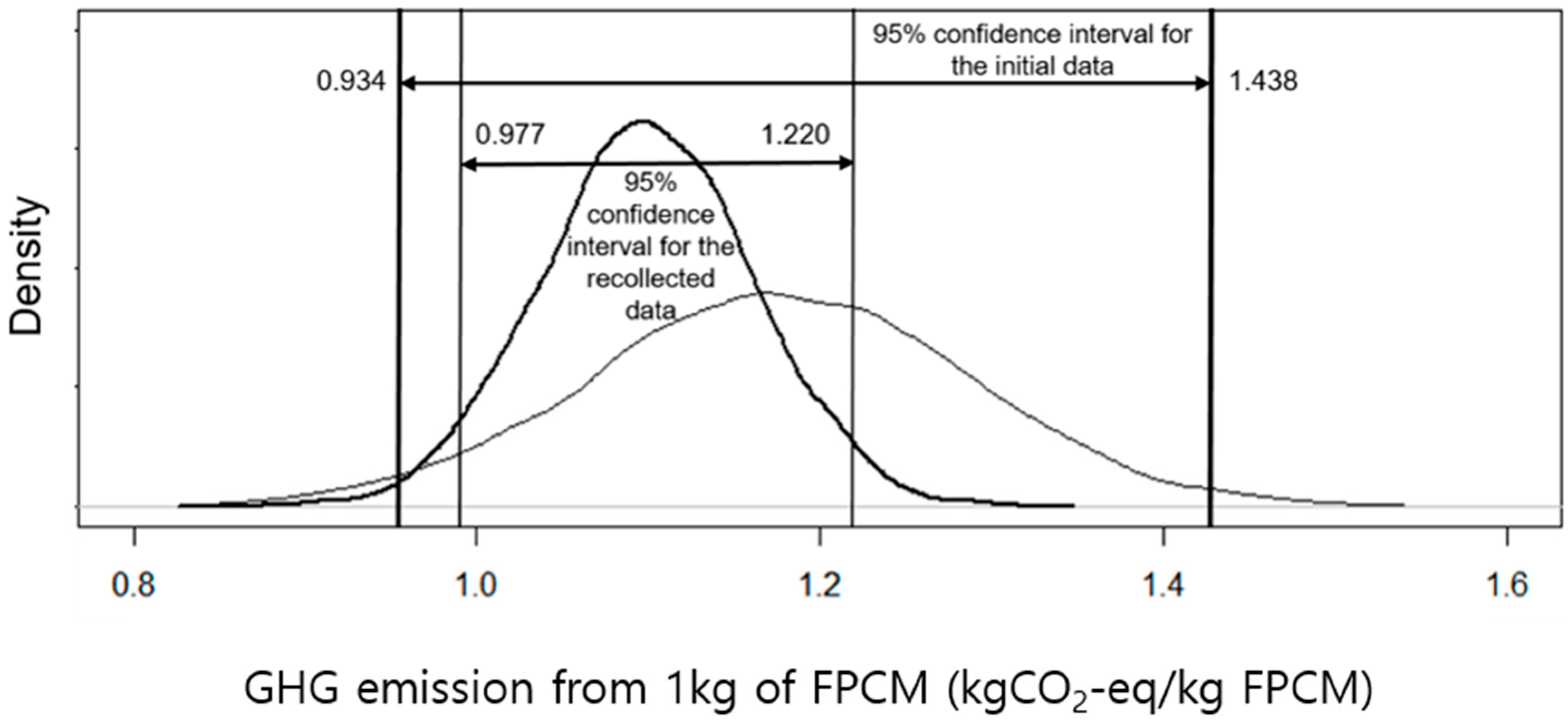
Figure 3 shows the PDF of the model output based on the initial data and the recollected data. The reduction in the interval length (upper bound–lower bound) from that of the initial dataset and the recollected dataset showed that the relative reduction of the interval length was 51.8%, whereas the relative reduction in the CV value was 47.6%. These results clearly indicate that the uncertainty of the model output was reduced significantly by the iteration of data collection of the problematic input variables.

Table 8. Result of the Monte Carlo simulation (MCS) for the total GHG emission from 1 kg of dairy cow FPCM.

	Before	After	Improvement (%)
Confidence interval (kg CO2–eq/kg FPCM)	0.934–1.438	0.977–1.220
Upper bound–lower bound	0.504	0.243	51.8%
CV (%)	10.76	5.64	47.6%

shows the MCS results for the total GHG emission for 1 kg of dairy cow FPCM.

Several uncertainty analysis studies for the GHG emissions from the dairy products used the MCS method [40,41,42]. However, there are differences in the methodologies of the uncertainty analysis between this study and others. The previous existing studies focused on estimating the uncertainty of the GHG emission itself from the dairy cow milk and estimating the PDF of the activity data from the literature or assumptions made by the experts. This study, however, identified the sources of the uncertainty, namely, the input variables contributing considerably to the uncertainty of the model output. On top of this, corrective measures were applied to reduce the error of the identified input variables by recollection of the data of the significant input variables. This result is the decreased uncertainty in the model output.

The identification of the input variables contributing considerably to the model output uncertainty was based on the calculation of the CTV of the input variables to the model output. To ensure proper selection of the input variables for iteration of data collection, the input variables exceeding a certain DQR value were selected for iteration of data collection. The assignment of a value to the element of the pedigree matric parameters based on the qualitative criterion is quite subjective, and one of the limitations of this study. We should collect more detailed data or go through more iterations.

However, the logic for including this qualitative approach was to reduce the effort required for the collection of the detailed data. As delineated in Step 5 in Figure 2, the DQR value calculation was used as a screening step for identifying input variables for iteration of data collection (detailed data). Clearly, the DQR approach used in this study should be improved or banned completely when there are other means available to use for choosing the input variables for iteration of data collection.

In addition, the K–S test was applied to estimate the PDF of the dataset of the selected input variables. A comparison of the uncertainty analysis method used in this study and the methods used by others is shown in

Table 9. Comparison of the uncertainty analysis methods.

Items	France [40]		New Zealand [41]	Sweden [42]	This Paper
	Conventional Farm	Organic Farm
Target for estimating uncertainty	Emission factors	Emission factors	Activity data and emission factors for direct emission from the farm	Activity data and Enteric fermentation factor	Activity data
Method for finding significant variables for the error	CTV analysis	CTV analysis	Regression coefficient	Variation of the data	CTV analysis and DQR
Key input variables for uncertainty of the GHG emission	Emission factors for manure deposited in pasture	Emission factors for manure deposited in pasture	Feed intake, EF3 1, EFCH4 2	Roughage feed intake, enteric CH4, energy use	Mixed feed intake, energy use, enteric CH4 from lactating cow
Tool for estimating uncertainty	Monte Carlo simulation	Monte Carlo simulation	Monte Carlo simulation	Monte Carlo simulation	Error propagation equation and Monte Carlo simulation
Method for determining PDFs	Literature and assumption	Literature and assumption	Assumption	Assumption	K–S test
Uncertainty reduction step	None	None	None	None	Yes (finding key variables, recollecting data, data quality assessment, etc.)
Data quality assessment method	None	None	None	None	DQR method
95% confidence interval (kg CO2–eq/kg FPCM)	1.024–1.052	1.037–1.126	0.745–1.197	0.94–1.33	0.977–1.220
Mean Value (kg CO2–eq/kg FPCM)	1.038	1.081	0.962	1.13	1.10
CV (%)	0.45	1.4	8.23	5.96	5.64

¹ emission factor for nitrous oxide due to excreta deposited during grazing, ² emission factor for methane emitted by the cows during digestion.

.

According to Table 9, the key input variables for uncertainty of the GHG emission are emission factors for manure deposited in pasture, feed intake, EF3, EF_CH4, energy use, and enteric GH₄ emission. It is difficult to compare directly the study in France to other studies, because the study in France was conducted on the error of the emission factor for calculating GHG emission directly from the farm. However, it has been shown that the calculation of emissions from manure treatment contributes to the uncertainty of the GHG emissions results. The CTV of the GHG emission from manure is 67% and 84% for conventional and organic farms, respectively. The reason for the uncertainty contribution to the manure management emission seems to be due to the difference in climate characteristics in the France area. The difference of the emission factors to be applied to the calculation of GHG emission by the manure management is considered to be due to the climate characteristics of the regions where dairy farms can operate.

Energy use has been identified as a key input variable in the case of Korea and Sweden. Both Korea and Sweden have four distinct seasons and seem to reflect the effect of these seasonal variations.

Table 9 shows that the CV value from the French study was lower than that from this study. In the French study, the number of dairy farms investigated including conventional and organic farms was 47, and the number of data points was 1692 over the three year period collected monthly (n = 47 × 12 × 3 = 1692).

The number of each data points in this study was 72, which came from one farm collected monthly for six years (n = 1 × 12 × 6 = 72). Differences in the number of data points may affect the variance of the input variables, such that the CV value was higher in this study compared to that in the French study. Meanwhile, the number of data points in the Swedish study, which exceeded 10,000, showed that the CV value was higher than that of the French study. This may indicate that the CV values may not be a reliable parameter for judging the reliability of the uncertainty analysis results.

Several uncertainty analysis studies in the LCA field employed the stochastic approach based on the assumed PDF or expert judgment [40,41,42]. Other studies in the case of the analytical approach ignored the PDF of the input variables completely [43,44]. Lack of PDF estimation or assumed PDF of the input variables may lead to poorer estimation of the variance of the input variables. This would adversely affect the reliability of the model’s uncertainty results.

Taking into consideration the above information, the proposed methodology in this study may be able to generate uncertainty results based on the limited number of data points. This is partly because the estimation of the PDF of the input variables was done in a systematic manner. This may allow us to estimate the variance of the input variables more reasonably, leading to a more reliable uncertainty analysis of the model output.

The contribution analysis for GHG emission is not a suitable method for finding key issues about the uncertainty of the results [7]. Therefore, it is a reasonable choice to identify significant input variables that require iteration of data collection through the CTV analysis and DQR.

The CTV analysis alone cannot lead to the selection of input variables for iteration of data collection, as the variance of a certain input variable cannot be reduced because of its innate nature. Sometimes, data quality can be inherently good (e.g., DQR <3) even if its CTV is high and in this case, iteration of data collection cannot improve its data quality. Therefore, the data quality analysis of the input variables identified from the CTV analysis is an essential element in reducing the uncertainty of the model.

However, there are shortcomings and disadvantages to the proposed uncertainty analysis method. These include the use of the pedigree-matrix for assessing data quality, and not considering the errors in the emission factors on the uncertainty results of the model output. Both the variance as well as the emission factors of the input variables influence the uncertainty of the model output in LCA [35,36,37]. The matrix-based approach considering both the variance of the input variable and its emission factor would be the viable alternative to the emission factor problem encountered in this study [13,29].

The Korean emission factors and the LCI database, however, have many shortcomings from a statistical standpoint, as such, emission factors were unreliable and thus not considered in this study. Accordingly, the matrix-based approach for LCA was not used in this study. The assignment of values to the elements of the pedigree-matrix based on the qualitative criterion is quite subjective and another shortcoming of this study.

4. Conclusions

An analytical and stochastic approach were used consecutively in the uncertainty analysis of the GHG emission model output. The error propagation equation and MCS method were used for the analytical and stochastic approaches.

An analytical approach can be an effective means for selecting input variables for the uncertainty analysis. A stochastic approach can prevent the risk of incorrect estimation of the uncertainty of the model output via PDF estimation and Monte Carlo simulation. This work showed that eliminating unnecessary iteration of data collection via the CTV analysis combined with the DQR calculation can increase the efficiency of the uncertainty analysis.

Application of the proposed procedure to a dairy cow milk farm showed that the uncertainty of the model output was reduced by the iteration of data collection of the input variables with a high CTV. This indicated that CTV analysis can be used to identify the input variables contributing considerably to the uncertainty of the model output. Investigating the data quality further reduced the number of input variables for iteration of data collection.

The use of the K–S test improved the estimation of the PDF of the datasets. A stochastic approach enabled more accurate quantification of the GHG emissions together with its uncertainty.

Finally, the study suggested an effective way to reduce the uncertainty of individual carbon footprint results by performing a series of steps to reduce uncertainty on activity data, input variables. The DQI for significant input variables derived through contribution to variance (CTV) was used as an index to evaluate the variance reduction potential of input variables. The uncertainty of the individual carbon footprint results was reduced through the iteration of data collection for input variables that could actually be improved.

The results of this study are expected to be useful as a way to manage the uncertainty of the results needed to ensure comparability of future environmental footprint results.

However, there are shortcomings and disadvantages to the proposed uncertainty analysis method. They include not considering the errors of the emission factors and upstream data on the uncertainty results and the use of the qualitative pedigree-matrix for assessing data quality. Future studies should address the contribution of the errors in the emission factors to the uncertainty of the model output. In addition, the use of the qualitative data quality analysis should be eliminated in future uncertainty analyses.

References

- Landi, D.; Capitanelli, A.; Germani, M. Ecodesign and Energy labelling: The role of virtual prototyping. Procedia CIRP 2017, 61, 87–92. [Google Scholar] [CrossRef]
- Favi, C.; Germani, M.; Landi, D.; Mengarelli, M.; Rossi, M. Comparative life cycle assessment of cooking appliances in Italian kitchens. J. Clean. Prod. 2018, 186, 430–449. [Google Scholar] [CrossRef]
- Du, C.; Dias, L.C.; Freire, F. Robust multi-criteria weighting in comparative LCA and S-LCA: A case study of sugarcane production in Brazil. J. Clean. Prod. 2019, 218, 708–717. [Google Scholar] [CrossRef]
- Food and Agriculture Organization of the United Nations (FAO). Greenhouse Gas Emissions from the Dairy Sector; FAO: Rome, Italy, 2010. [Google Scholar]
- Ministry of Environment Korea. The Framework Act on Low Carbon, Green Growth; Ministry of Environment Korea: Seoul, Korea, 2013.
- Ministry of Environment Korea. The Act on the Allocation and Trading of Greenhouse Gas Emission Permits; Ministry of Environment Korea: Seoul, Korea, 2012.
- Lee, M.H.; Lee, J.S.; Lee, J.Y.; Kim, Y.H.; Park, Y.S.; Lee, K.M. Uncertainty Analysis of a GHG Emission Model Output Using the Block Bootstrap and Monte Carlo Simulation. Sustainability 2017, 9, 1522. [Google Scholar] [CrossRef]
- De Camillis, C.; Bauer, C.; Schenker, U.; Martin, N. ENVIFOOD Protocol Environmental Assessment of Food and Drink Protocol; European Food Sustainable Consumption and Production (SCP) Round Table, Working Group 1: Brussels, Belgium, 2013. [Google Scholar]
- European Union. Commission Recommendation of 9 April 2013, on the Use of Common Methods to Measure and Communicate the Life Cycle Environmental Performance of Products and Organisations; European Union: Brussels, Belgium, 2013. [Google Scholar]
- Kauffman, J.; Lee, K.-M. Handbook of Sustainable Engineering; Springer: Berlin/Heidelberg, Germany, 2013; pp. 371–388. [Google Scholar]
- Der Kiureghian, A.; Ditlevsen, O. Aleatory or epistemic? Does it matter? Struct. Saf. 2013, 31, 105–112. [Google Scholar] [CrossRef]
- Saltelli, A.; Ratto, M.; Andres, T.; Campolongo, F.; Cariboni, J.; Gatelli, D.; Saisana, M.; Tarantola, S. Global Sensitivity Analysis: The Primer; John Wiley & Sons: Hoboken, NJ, USA, 2008. [Google Scholar]
- Heijungs, R.; Suh, S. The Computational Structure of Life Cycle Assessment; Springer Science & Business Media: New York, NY, USA, 2002. [Google Scholar]
- Heijungs, R.; Lenzen, M. Error propagation methods for LCA—A comparison. Int. J. Life Cycle Assess 2014, 19, 1445–1461. [Google Scholar] [CrossRef]
- Uwizeye, A.; Gerber, P.J.; Groen, E.A.; Dolman, M.A.; Schulte, R.P.; De Boer, I.J. Selective improvement of global datasets for the computation of locally relevant environmental indicators: A method based on global sensitivity analysis. Environ. Modell Softw. 2017, 96, 58–67. [Google Scholar] [CrossRef]
- Heijungs, R. Identification of key issues for further investigation in improving the reliability of life-cycle assessments. J. Clean. Prod. 1996, 4, 159–166. [Google Scholar] [CrossRef] [Green Version]
- Williams, E.D.; Weber, C.L.; Hawkins, T.R. Hybrid Framework for Managing Uncertainty in Life Cycle Inventories. J. Ind. Ecol. 2009, 13, 928–944. [Google Scholar] [CrossRef]
- Easton, V.J.; John, H. McColl, 2004. Statistic Glossary v 1.1. Available online: http://www.stats.gla.ac.uk/steps/glossary/index.html (accessed on 24 January 2019).
- Sobol’, I.M. Sensitivity Analysis for nonlinear mathematical models. Math. Modeling Comput. Exp. 1993, 4, 407–414. [Google Scholar]
- Homma, T.; Saltelli, A. Importance measures in global sensitivity analysis of nonlinear models. Reliab. Eng. Syst. Saf. 1996, 52, 1–17. [Google Scholar] [CrossRef]
- Saltelli, A.; Chan, K.; Scott, E.M. Sensitivity Analysis; Wiley: New York, NY, USA, 2000. [Google Scholar]
- Baek, C.-Y.; Lee, K.-M.; Park, K.-H. Quantification and control of the greenhouse gas emissions from a dairy cow system. J. Clean. Prod. 2014, 70, 50–60. [Google Scholar] [CrossRef]
- Henriksson, P.J.G.; Guinée, J.B.; Heijungs, R.; de Koning, A.; Green, D.M. A protocol for horizontal averaging of unit process data—Including estimates for uncertainty. Int. J. Life Cycle Assess 2014, 19, 429–436. [Google Scholar] [CrossRef]
- Lee, K.M.; Park, K.H. Development of Carbon Tracing System for Livestock Agriculture: Development of LCI DB and Estimation of Greenhouse Gas from Feedstuff Research Report; National Institute of Animal Science of the Republic of Korea: Seoul, Korea, 2012.
- Saltelli, A. Global sensitivity analysis: An introduction. In Proceedings of the 4th International Conference on Sensitivity Analysis of Model Output, (SAMO’04), Santa Fe, NM, USA, 8–11 March 2004; pp. 27–43. [Google Scholar]
- Huijbregts, M.A.; Norris, G.; Bretz, R.; Ciroth, A.; Maurice, B.; von Bahr, B.; Weidema, B.; de Beaufort, A.S. Framework for modelling data uncertainty in life cycle inventories. Int. J. Life Cycle Assess 2001, 6, 127–132. [Google Scholar] [CrossRef]
- Bevington, P.R.; Robinson, D.K. Data Reduction and Error Analysis; McGraw-Hill: New York, NY, USA, 2003. [Google Scholar]
- Zehetmeier, M.; Baudracco, J.; Hoffmann, H.; Heißenhuber, A. Does increasing milk yield per cow reduce greenhouse gas emissions? A system approach. Animal 2012, 6, 154–166. [Google Scholar] [CrossRef] [PubMed]
- Groen, E.; Heijungs, R.; Bokkers, E.; de Boer, I. Methods for uncertainty propagation in life cycle assessment. Environ. Model. Softw. 2014, 62, 316–325. [Google Scholar] [CrossRef]
- Heijungs, R. Sensitivity coefficients for matrix-based LCA. Int. J. Life Cycle Assess 2010, 15, 511–520. [Google Scholar] [CrossRef] [Green Version]
- Intergovernmental Panel on Climate Change. 2006 IPCC Guidelines for National Greenhouse Gas Inventories; Intergovernmental Panel on Climate Change: Geneva, Switzerland, 2006. [Google Scholar]
- Weidema, B.P.; Wesnæs, M.S. Data quality management for life cycle inventories—An example of using data quality indicators. J. Clean. Prod. 1996, 4, 167–174. [Google Scholar] [CrossRef]
- International Organization for Standardization. ISO 14067:2018—Carbon Footprint of Products—Requirements and Guidelines for Quantification; International Organization for Standardization: Geneva, Switzerland, 2018. [Google Scholar]
- Wang, E.; Shen, Z. A hybrid Data Quality Indicator and statistical method for improving uncertainty analysis in LCA of complex system–application to the whole-building embodied energy analysis. J. Clean. Prod. 2013, 43, 166–173. [Google Scholar] [CrossRef]
- Everitt, B. Cambridge Dictionary of Statistics; Cambridge University Press: Cambridge, UK, 1998. [Google Scholar]
- Natrella, M. Engineering Statistics Handbook, National Institute of Standards and Technology. 2013. Available online: http://www.itl.nist.gov/div898/handbook/index.htm (accessed on 11 December 2018).
- Ross, S.M. Introduction to Probability and Statistics for Engineers and Scientist, 4th ed.; Academic Press: Waltham, MA, USA, 2009. [Google Scholar]
- Zaiontz, C. Real Statistics Using Excel. 2014. Available online: http://www.real-statistics.com/tests-normality-and-symmetry/statistical-tests-normality-symmetry/kolmogorov-smirnov-test/ (accessed on 24 January 2019).
- Pham, H. Springer Handbook of Engineering Statistics; Springer Science & Business Media: New York, NY, USA, 2006. [Google Scholar]
- Chen, X.; Corson, M.S. Influence of emission-factor uncertainty and farm-characteristic variability in LCA estimates of environmental impacts of French dairy farms. J. Clean. Prod. 2014, 81, 150–157. [Google Scholar] [CrossRef]
- Basset-Mens, C.; Kelliher, F.M.; Ledgard, S.; Cox, N. Uncertainty of global warming potential for milk production on a New Zealand farm and implications for decision making. Int. J. Life Cycle Assess 2009, 14, 630–638. [Google Scholar] [CrossRef] [Green Version]
- Henriksson, M.; Flysjö, A.; Cederberg, C.; Swensson, C. Variation in carbon footprint of milk due to management differences between Swedish dairy farms. Animal 2011, 5, 1474–1484. [Google Scholar] [CrossRef] [PubMed] [Green Version]
- Hong, J.; Shaked, S.; Rosenbaum, R.K.; Jolliet, O. Analytical uncertainty propagation in life cycle inventory and impact assessment: Application to an automobile front panel. Int. J. Life Cycle Assess 2010, 15, 499–510. [Google Scholar] [CrossRef]
- Imbeault-Tétreault, H.; Jolliet, O.; Deschênes, L.; Rosenbaum, R.K. Analytical propagation of uncertainty in life cycle assessment using matrix formulation. J. Ind. Ecol. 2013, 17, 485–492. [Google Scholar] [CrossRef]
Figure 1.
System boundary diagram for the study.
Figure 2.
Proposed step-by-step procedure for the uncertainty analysis.
Figure 3.
Result of the Monte Carlo simulation for the GHG emission from 1 kg dairy cow FPCM.