Interaction of Public Transport Accessibility and Residential Property Values Using Smart Card Data


1
Research Centre for Integrated Transport Innnovation (rCIIT), UNSW Sydney, Sydney 2035, Australia
2
School of Civil Engineering, University of Sydney, Sydney 2006, Australia
*
Author to whom correspondence should be addressed.
Sustainability 2019, 11(9), 2709; https://doi.org/10.3390/su11092709
Submission received: 12 April 2019
/
Revised: 1 May 2019
/
Accepted: 5 May 2019
/
Published: 13 May 2019
(This article belongs to the Section Sustainable Transportation)
Abstract
:This study examines the relationship between residential property values and accessibility indicators derived from transit smart card data. The use of smart card data to estimate accessibility indicators for explaining the housing market has not yet been explored in the literature. Hence, this paper employs information from Brisbane, Australia’s “go card” and corresponding property data to develop residential property hedonic pricing models using an ordinary least square (OLS) model, a spatial lagged model (SL), a spatial error model (SE), and a geographically weighted regression (GWR). Due to the systematic coincidence between location and price similarities, these spatial econometric models yield superior goodness-of-fit over the OLS model. Using the proposed definition of public transit accessibility in this study, it was found that properties located in well-connected, well-serviced, and accessible locations generally experience premiums in their values. The results indicate that there is value added to the property market from the public investment in public transport services and infrastructure, which supports the adoption of transit funding mechanisms, such as value-capture taxes. Furthermore, the analysis of spatial interactions between transport accessibility and the housing market could be of use to policy makers to ensure a just distribution of capital investment in future infrastructure projects.
1. Introduction
Public transit can bring about benefits as well as negative externalities to nearby residents. On one hand, transit can improve accessibility, reduce congestion, foster urban growth, and even cause an uplift in surrounding properties’ values. On the other hand, communities often push back on transit due to high price tags [1,2], competition for limited space particularly regarding street parking [3], reduced quality of life in the property due to air or noise pollution, and public perception of public transit users [4,5,6].
Many studies have examined the positive and negative relationships between property values and various accessibility indicators due to new or existing public transport infrastructure [7,8,9,10,11,12]. Using Brisbane as an example, Levinson et al. [13] reported that, two years after opening the first segment of 16.9 km of Brisbane’s South East Busway serving 60,000 daily commuters, it attracted three major development projects, as well as causing a 20% growth in residential land values within walking distance to stations. Moreover, major transportation investments, such as the Brisbane busway system, are generally expensive, and their costs often preclude their construction if they rely on fares alone for funding [14]. Hence, by identifying the relationship between accessibility indicators and property value increases due to public investment, policy makers can better capture the full value of public transit and leverage it to fund the investment.
While the aforementioned studies investigated the effects of new and existing public transportation infrastructures on property values using either Euclidean or network distances to different types of transit stations to measure accessibility, none have investigated property-specific associations of public transport usage to explain property values. In the past, extensive public transport usage data have been difficult to collect due to privacy limitations and costs. However, the introduction of smart card ticketing systems has enabled public transport operators to gather more detailed information on each individual passenger regarding their travel behaviour and some level of travellers’ characteristics. When the smart card data are analysed in aggregate this allows operators to adjust their services and identify new service opportunities [15]. This paper employs public transit usage data from the electronic ticketing system in Brisbane, Australia (go card) to establish accessibility indicators and explore their impacts on property values. To find those underlying relationships, several spatial regression approaches were employed to produce a comprehensive comparison between the approaches and their results.
This paper examines the relationships between public transport accessibility and property values using data from Brisbane, Australia as a case study. The public transport accessibility indicators used in this study are designed to capture the accessibility experienced by residents and provide an alternative from the traditional definition of public transit accessibility, where only the spatial dimension is considered. Another contribution of this study is to show the potential of smart card data to develop accessibility indicators for hedonic pricing models in this domain of research.
The following sections present an overview of the literature, the key details of the study area (Brisbane, Australia), and the public transit usage data. Section 4 details the methodology, followed by Section 5 presenting the results and a detailed discussion about the findings. Section 6 provides a discussion of the policy implications and some concluding remarks.
2. Literature Review
Accessibility and land values are closely related factors influencing housing demand. Being close to major transport infrastructure, such as a highway or a public transport station, generally yields a high level of accessibility, and property prices around such locations often come with a premium. There are nuances in the relationship as residents recognize differences in the quality of the transport services and respond with their willingness to pay. Transit nodes (bus stops, train stations, ferry wharves, etc.) are characterized by the diversity of route options, service frequency, connectivity to the larger transit network, travel time reliability, travel cost, comfort, multimodality, security, and ease of access or egress. Hence, real estate around ‘better’ public transport stations and stops is expected to inherit a greater premium compare to those near low-quality transport. In the field of hedonic modelling, accessibility is commonly introduced into the equation as either the travel time or distance to the central business district (CBD) or to the nearest transit station or stop [16,17,18,19,20]. Whereas in the domain of interaction of public transport accessibility and property prices, the literature has not previously explored how the heterogeneity of public transport nodes may affect the premium on nearby properties.
2.1. Urban Economics
The determination of a premium on property values near high quality public transit nodes is a lens for examining the relationship between accessibility and residential location selection. Accessibility plays an important role as one of the main determinants of property value. Von Thünen [21] provided a foundation for urban economics in which he theorised an inverse relationship between transportation costs and land cost under his farmland and market city assumptions. A century later, Alonso [22] extended the work of Von Thünen to demonstrate a trade-off between the cost of commuting and housing cost, known as bid rent function theory. Therefore, to live closer to CBD with greater accessibility to services and job locations, people are forced to spend more on housing costs and as a result, their spending on commuting costs will become less. Capitalising on this willingness to pay, accessible locations have higher potential for development in the eyes of land developers. The history of the recognition of the linkage between accessibility and property values has been further supported in many modern studies of urban property value [9,23,24,25,26]. However, not all empirical studies found that properties near public transit exhibit a premium due to possible negative externalities (e.g., crime and noise). As an example, a recent study by Mulley et al. [12] found that properties within 50 metres to a rail station have a price discount of 7.7% and crime also negatively correlates with the distance to a rail station, in general. It should be noted that the definition of public transport accessibility is generally limited to the closest distance or time to different types of public transport services, which may not reflect the accessibility that those services actually provide to nearby residents. Hence, it is the focus of this study to explore the kind of accessibility which is oriented toward the resident use of the system rather than just the spatial dimension of accessibility alone.
2.2. Hedonic Price Models
Hedonic price modelling determines the implicit price of housing, where determinants are, generally, housing structural, locational, and neighbourhood-related attributes. Lancaster [27] reasoned that goods are not direct objects of utility but their attributes confer utility. Rosen [28] proposed how this approach can be applied in modelling the implicit price of housing based on the characteristics of the house. However, there are several empirical issues with the early hedonic price models, notably the use of an inappropriate functional form to represent the relationship between the attributes and commodity prices, which may result in inconsistent estimates [29]. Building on methodological improvements, a vast number of studies explored the implicit value of various accessibility measures to residential property values [9,23,24,25,26,30,31,32,33,34]. Hedonic price models are usually carried out using linear regression methods, and some more recent studies utilise advanced regression approaches, such as spatial regression approaches and geographically weight regression (GWR) approaches [35,36,37]. Spatial error and spatial lag models are suitable if the OLS regression residuals are found to be spatially dependent. A spatial error linear regression model considers unobserved correlated errors based on a spatial relationship between observations. Similarly, a spatial lag linear regression model is specified based on the idea “like attracts like”, meaning that in a real estate context, houses that are nearby often share a similar price. Hence, the price of one house can often be partially explained by the prices of its neighbours based on a specified spatial relationship between them or, in other words, it accounts for spatial dependence effects. In contrast, GWR allows the regression coefficients to be locally estimated based on the spatial relationship among observations while ensuring that, if spatial heterogeneity exists in the regression parameters, their estimates will not be biased [38]. This approach is often found useful in cases where relationships between the dependent variable and independent variables vary significantly over space, such as in ecological systems and land use studies. Through GWR, planners can make locally appropriate policy recommendations that capitalise on the spatially varying relationships between property values and the determinants.
2.3. Smart Card
Given the focus on experienced accessibility (i.e., the accessibility benefit experienced by the resident of the property), it is crucial that the right kind of data is available to evaluate the proposed resident-oriented public transport accessibility indicators. The data must reveal how people who live in properties near public transport nodes use the services. The introduction of smart card ticketing systems has not only increased convenience, efficiency, and integration of services for public transit users, but also paved the way for more advanced transport research. Through the technology, detailed user travel data can be collected at a much lower cost as compared to direct survey methods. Although smart card data may not yet completely replace direct travel survey methods due to missing information, such as the journey purpose [39], it offers a comprehensive view of how residents access the public transit system. Due to confidentiality and privacy concerns around the use of smart card data, these datasets are generally unavailable to the public and often difficult even for researchers to obtain. Nonetheless, in recent years, there have been several studies which explored the use of smart card data for various purposes: Agard et al. [40] attempted to obtain user travel behaviours by data mining smart card data; Morency et al. [41] showed that smart-card data can be used to measure the spatial and temporal variability of transit use to create a travel profile for different types of card owners; Devillaine et al. [42] used smart card data along with land use and user behaviour data to identify trip purposes; and Wei et al. [15] demonstrated the relationship between the commuting patterns of public transport passengers and land use patterns using smart card data. Most of the research around the use of smart card data has been done in the hope to better understand user travel behaviour, but none has attempted to link this emerging data source with hedonic pricing methodologies.
Two main literature gaps therefore exist. First, on the impact of resident-oriented, heterogeneous accessibility on property values. Second, on the use of public transport smart card data in developing accessibility measures to be used in the domain of the interaction of public transport accessibility and property prices. The paper addresses these gaps concurrently. The next section introduces the study area, Brisbane, Australia, and the data involved, followed by the methodology, results and discussion, and conclusion and policy implications.
3. Study Area and Data
3.1. Study Area
Brisbane is one of the major Australian cities. It is a city of 2.3 million people [43], which is about half of Sydney or Melbourne. The Brisbane River divides the city into North and South Brisbane with the CBD located in one of the river bends. Brisbane has a wide range of public transport services, including bus, rail, and ferry. These services are provided mainly by Brisbane Transport, which was corporatized by the Brisbane city council in 1990. As of 2013, Brisbane city has 12 train lines, 6 ferry lines, and more than 450 bus routes operating in and around the city area. From the 2011 Australian Census of Population and Housing, there was a considerable shift in the number of people who travelled to work using public transport and active transport modes, such as walking and cycling. Specifically, for people who worked in the CBD area, this shift increased from 59.3% to 63.2% between 2006 and 2011, which was more than twice compared to those who travelled to work by a private vehicle of 28.7% in 2011 [44]. In the bigger picture, as reported by the Department of Transport and Main Roads of Queensland [45], the majority of Greater Brisbane travel occurs during off-peak times, which accounts for 59%, followed by 23% in the AM peak and 18% in the PM peak. Together, Brisbane residents make 6.3 million trips each weekday across all available transport options. Commuting to work consumes the most time-spent (32 min) and is the longest distance (15.1 km) on average compared to other regular activities. City-wide, private vehicle as driver is the dominant travel choice by Brisbane residents, followed by private vehicle as passenger. Public transport accounted for 10% of the mode choice as did walking, whereas cycling was only 1%.
3.2. Property Data
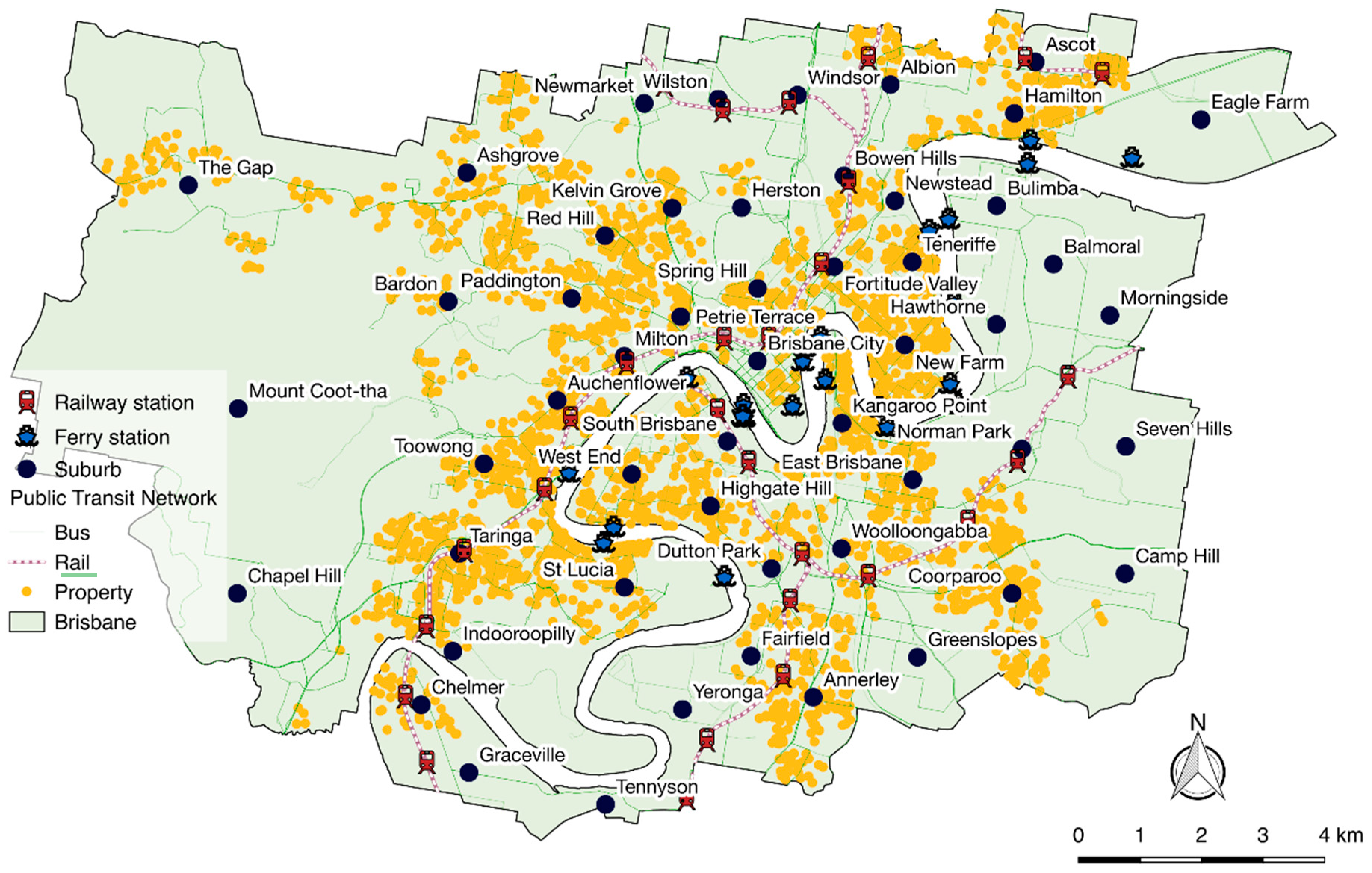
The study contains 5406 property transaction records from the year 2013 collected by corelogic.com.au across the Greater Brisbane region (see Figure 1). Each record comes with the property value and its internal and spatial features, such as the number of bedrooms, the number of bathrooms, car space, address, geographical coordinates, etc. Please refer to Table 1 for descriptive statistics. Unfortunately, property details, such as the lot size, floor area, structural condition, and age of the property—which have been found to be significant in the literature—were not available. To control temporal effects, both the property data and the smart card data were both from the same year, 2013.
3.3. Go Card Data
The go card electronic ticketing system was first introduced in 2008 to replace independent fare systems on all TransLink’s transportation services in South Queensland, Australia. In this study, go card data were collected by TransLink, an agency of the Department of Transport and Mains Roads in Queensland, for a period of one-day, on 1 March 2013 (Friday). Over 600,000 trip records were collected during that day. Each record contains trip ID, journey ID, route ID, service ID, direction, card type, boarding time, alighting time, boarding stop alighting stop, amongst other information (see Table 1). However, the unique user and card type are not available due to passenger privacy concerns. Although the exact geographical location of each stop was not given with the data, it can be matched with General Transit Feed Specification (GTFS) data to obtain its geographical coordinates.
3.4. Neighbourhood Statistics
The Australia Bureau of Statistics (ABS) provides access to a wide range of population and housing statistics from the past census surveys. Neighbourhood statistics can be obtained from the 2011 Population and Housing Census survey (available on http://www.abs.gov.au/census). In this study, each property is linked to its associated SA1 (statistical area 1) neighbourhood statistical features, where the population size of each SA1 is generally around 200 to 800 residents [46].
3.5. Employment
The employment in each neighbourhood was estimated using the place of work statistics which was obtained from ABS as reported in the 2011 Population and Housing Census survey. This statistic was used to estimate the job accessibility indicator. The most detailed resolution available for employment statistics is the DZ (destination zone). By comparison, the DZ is slightly larger than statistical area 1, but smaller than statistical area 2 (for more information, please refer to [46]).
4. Methodology
To explore possible relationships between property values, which are the dependent variable, and accessibility indicators, property features, and neighbourhood characteristics, this study employed four types of regression techniques: Ordinary least squares (OLS), spatial lag (SL), spatial error (SE), and geographically weighted regression (GWR). The latter three techniques provide more suitable formulations that capture spatial dependency where an OLS regression falls short.
4.1. Extraction of Accessibility Indicators from Go Card
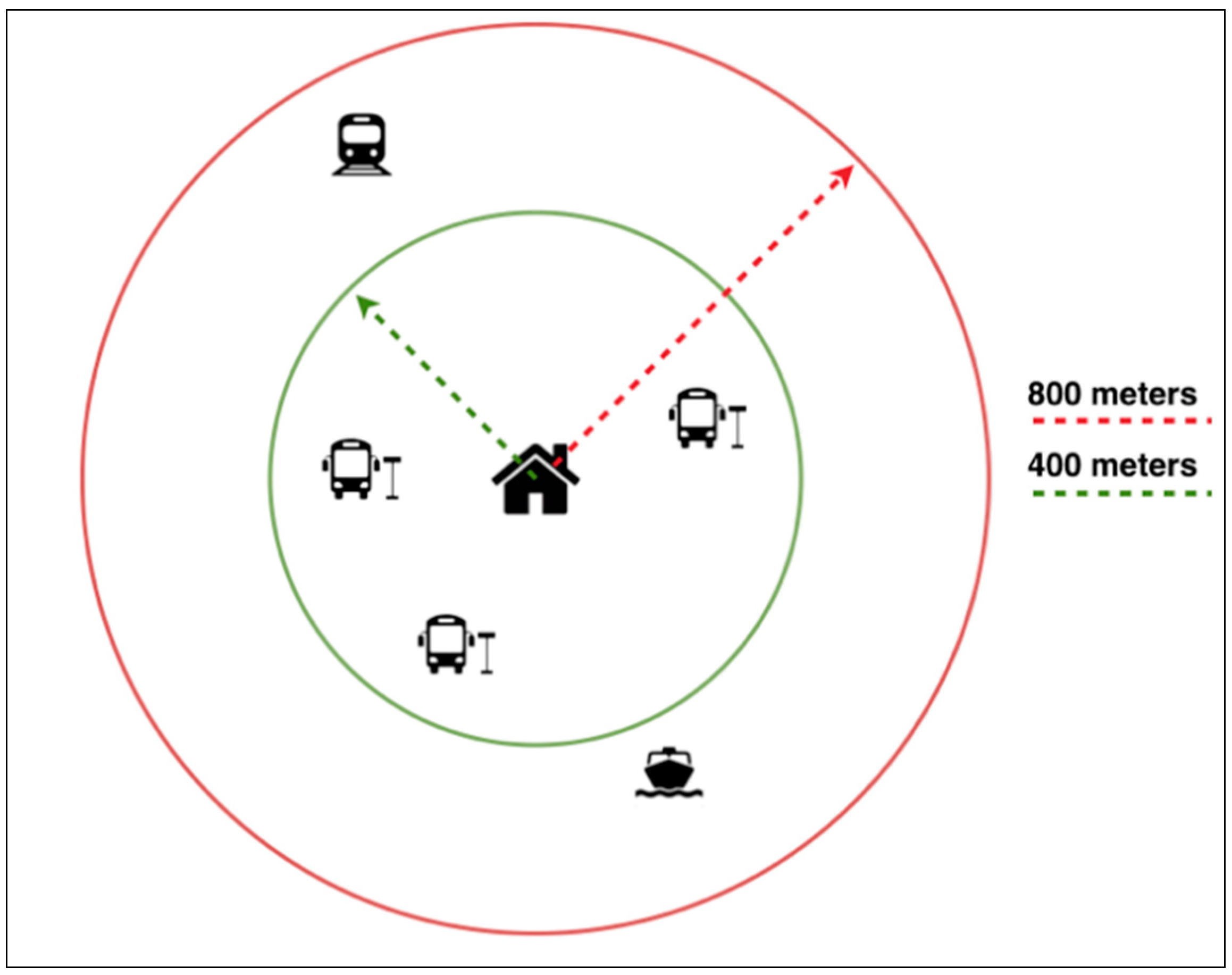
The objective here was to construct accessibility indicators which help to capture transit nodes. Hence, using the go card data, various transit accessibility indicators can be evaluated, such as the total number of trips originating and alighting at a station, the total number of transfers made, the average travel time, the average delay, the waiting time of transfer trips, the number of trips to the CBD, etc. Although this study focuses on ease of travel from the perspective of the property owners, there is no simple solution to identify which transit nodes are used by them. Hence, for every property record, aggregate accessibility indicators of all bus stops within a 400 m circular buffer and all railway stations and ferry stations within 800 m of each property were considered. The buffer distances were assumed based on the current practice to define transit catchment areas [47,48,49,50], irrespective of the geographical setting and pedestrian environment, which may affect the walkability around each property. This assumption could be further improved in future studies using findings from walkability studies of the study area.
Travel time is one of the predominant costs of transport. Travel time variability can be interpreted as a loss in economic productivity. In the long term, the effects of traffic congestion can alter the land-use pattern of a city as illustrated by the shrinkage of business market areas of the city [51]. Hence, travel time variability reflects the cost due to unreliable transport service. In Equation (1), the travel time variability of station i is calculated as the standard deviation of the travel time between a boarding station, i, to each alighting station, j, using only those station pairs with more than 15 trips. The travel time variability variable was linked to each associated property by averaging the variability for all stations, i, within the catchments described in Figure 2.
The delay indicator of a station, used in this study, was defined as the average normalised difference between the 85th percentile travel time and the median travel time of all departing trips between station i to all stations j, denoted as N, where N represents a set of stations with at least 15 departing trips between the origin-destination pair (see Equation (2)). This indicator represents the reliability of the public transport services people experienced from their nearby public transportation services.
The number of trips departing from each station represents the total ridership at each station and it gives a deeper sense of how important a transit station, or a stop, is to the nearby residents. The ridership was extracted for morning peak hours, 06:00 to 09:00, and the evening peak hours, 15:00 to 18:00. These two periods captured commuting trips made by most people, focusing on home to work or school and work or school to home, respectively.
Brisbane’s CBD is the most visited destination for public transport users. The number of trips to the CBD was calculated by adding all journeys ended or transferred at a station or stop located within Brisbane’s CBD. Some public transport passengers who live in areas less-connected to major employment areas, recreational areas, or central transport hubs may need to make more transfers on average than those living in well-connected areas, such as the CBD. On the other hand, zones with higher numbers of transfer trips may seem to have better connectivity to other zones. The transfer indicator used in this study was calculated using the proportion of departing trips containing at least one transfer for all the stations in the transit catchment to each property, as shown in Figure 2.
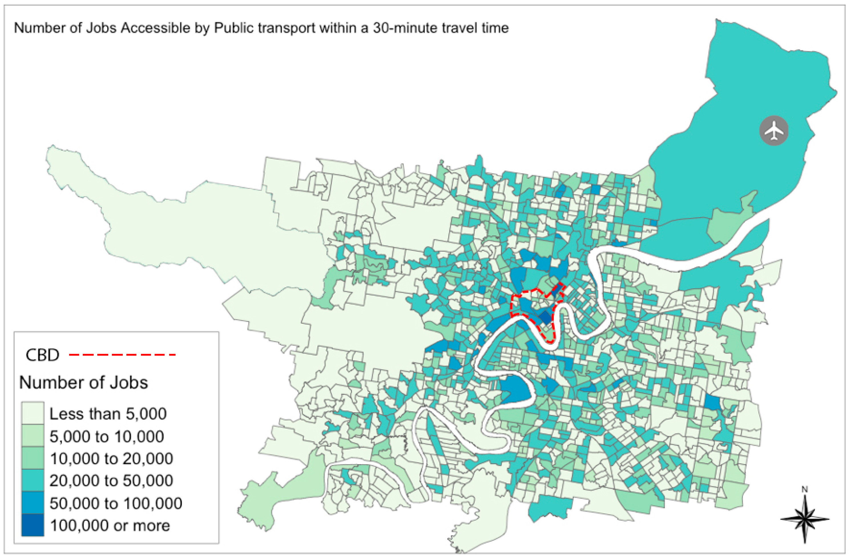
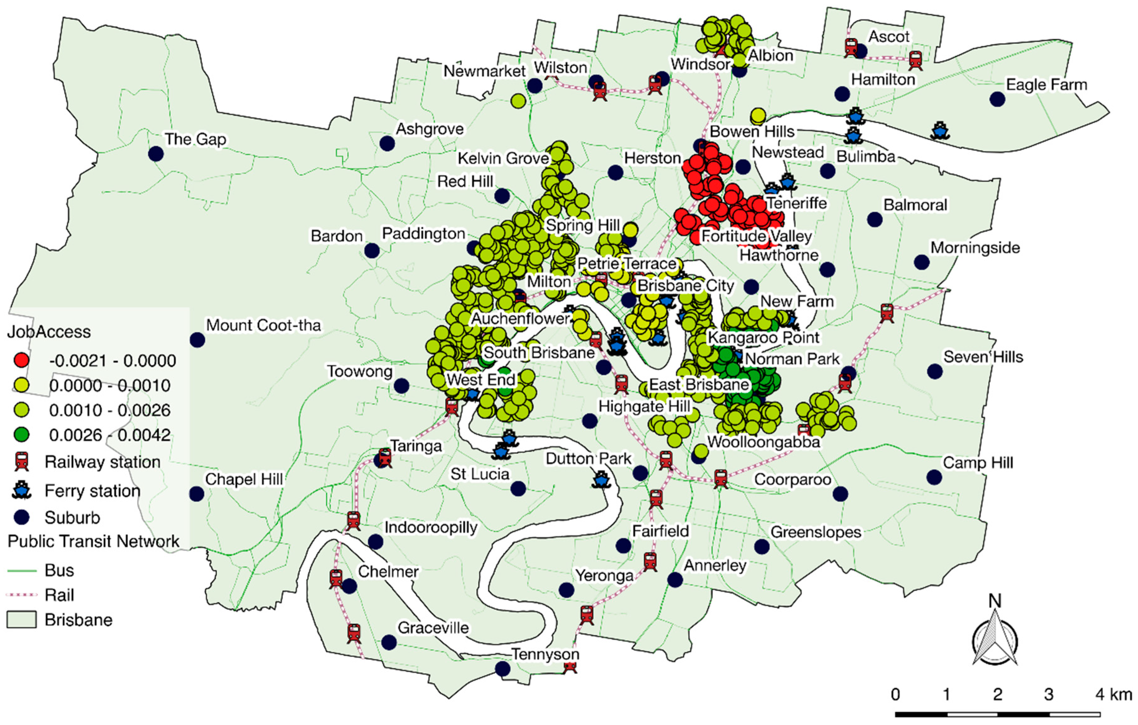
One additional indicator that was included in this study is the number of jobs accessible from public transport services within a 30-min journey, on average, (a journey can contain multiple trips) from each SA1 (statistical area level 1) zone. In Greater Brisbane, work commutes take on average 32 min [45]. Place of work statistics at different geographical boundaries can be found on the Australia Bureau of Statistics (ABS) website. Using both data, we derived an employment accessibility indicator by the public transport from each zone, and the result is shown in Figure 3.
4.2. Model Specification
In Equation (3), property value is the dependent variable, with a set of explanatory variables on the right hand-side of the equation. , , and are vectors representing characteristics of the property, the neighbourhood’s characteristics, and the public transit accessibility indicators, respectively (see Table 2)., , and are vectors of coefficients for each category, in the same order. is the Gaussian error vector. The model is estimated in a semi-log specification to deal with non-linearity and enables a simple interpretation of the effect from the model’s coefficients as price elasticities.
The internal features of the property, used in this study, are the number of bedrooms, the number of bathrooms, the number of car spaces, and its structural type (unit or house). However, given the property data available at the time, not all important features were reported by the source, such as the floor size of the property, the property’s age, and the parcel size of the property, which were found to be significant in other related hedonic pricing studies.
The neighbourhood features that were linked to each property record are the percentage of persons with a weekly income of more than $1500, percentage of persons aged more than 65-years, population density, and one-year migration ratio. These variables were found to be significant factors that explained the variations in property values from other studies, such as a study by [26], which explored the premiums on properties based on the proximity to ferry stations in Brisbane, Australia.
The accessibility indicators extracted from the smart card data included the number of trips during morning peak hours (OMP); the number of trips during evening peak hours (OEP); the number of trips to the CBD (CBDTrips); the ratio between the departing trips, which involved at least one transfer, to the total number of departing trips (NTF); and the job accessibility indicator (JobAccess). Note that these variables are what makes this study unique since they introduce the residents’ use of the system rather than just the spatial dimension of accessibility alone while being consistent with the conventional measures of transit accessibility used elsewhere.
It should be pointed out that, in the model selection phase, we tested 23 other accessibility indicators, such as transfer time, travel time, and time-specific origin and destination demands, using the smart card data, but only those ones that we present here in the paper were found to be significant and have an acceptable level of multicollinearity.
The remaining accessibility indicators were evaluated using geographical information using the conventional measures of transit accessibility. Each property has two dummy variables to indicate whether it is close to a rail station (Rail400) and/or a ferry station (Ferry800). The number of bus stations and stops within a 400 m radius to each property (Bus) was also included as an accessibility indicator. The network distance from the centroid of the SA1 to the CBD (CBD) was also included, and Google Maps API was used to retrieve the distances.
4.3. Spatial Regression Models
Spatial correlation implies that observations that are spatially close to each other have more similarity than those further away, therefore, they can sometimes be used to infer about their neighbours. Hence, a spatial lag and spatial error models were employed to mitigate the presence of spatial dependence that could violate OLS assumptions.
To capture these interactions, the SL model is expressed as follows:
where is the strength of the spatial correlation, is a n-by-n matrix with zeroes along the diagonal indicating the spatial relationships between different observations, is an n-by-1 vector of the spatial lag of the dependent variable, and the rest are as previously defined.
The second model is spatial error (SE), a regression method for correcting the spatial autocorrelation within spatial data due to unobservable factors or omitted variables associated with the location [52]. The SE regression model can be expressed as:
In this model, the error term, , has a spatial structure where the errors are spatially correlated. is the spatial error coefficient and is a vector which represents well-behaved, spatially uncorrelated errors.
To construct both models, a spatial weights matrix must be defined by assuming the spatial relationship between the observations. There are several ways to define the spatial relationship, such as basing it on distance and contiguity. For a distance-based spatial matrix, the spatial relationship is defined either by Euclidean [53] or road network [54] distance. As one would expect, the method which is used to construct the spatial weight matrix will pose a significant impact on the outcome of the model. In this study, the spatial weight relationship between each pair of properties, , was calculated using a bi-square weighting function:
where is the Euclidean distance between property i and property j, d denotes the maximum distance between the properties to have a spatial influence greater than 0. An 800-m threshold, , was used as it was found to be the optimal result, compared to using the log likelihood values of spatial error models with a varying threshold from 100 m to 3 km. Once the spatial weight matrix was constructed, the matrix was then row-standardized, hence each row sums to one.
The ‘spdep’ package created by Roger Bivand et al. [55,56] implemented in R language [57] was used to create the spatial regression models. The ‘spdep’ package provides spatial regression modelling tools for estimation and testing, as well as functions to create a spatial weight matrix. Further reading on these approaches and derivations of the spatial parameters can be found in [58,59].
4.4. Geographically Weighted Regression (GWR) Approach
The GWR [60] method is often used when dealing with non-stationarity in relationships over space. Hence, use of the GWR method allows us to capture spatially varying relationships between the dependent and independent variables in a spatially disaggregate manner instead of considering them to be constant over space. However, GWR does not solve misspecification problems nor specifically address spatially auto-correlated residuals, but one may justify a need for GWR if spatial autocorrelation in residuals of an OLS model with spatial data is observed. Building on the traditional regression framework, a basic GWR can be expressed as:
where represents the natural log of the property value at location i, is the value of the explanatory variable, k, at location i, and are geographical coordinates of location i, is the intercept parameter at location i, is the local regression coefficient at location i, and the error term, , is the Gaussian error at location i. A modified ordinary least squares algorithm which incorporates spatial weights was applied to estimate the local relationships between property values and a set of explanatory variables in the form expressed above. In contrast to an OLS regression model, where coefficients represent the global or overall relationships, the GWR coefficient values of each independent variable are location dependent values.
However, before the local coefficients can be estimated, the bandwidth of the spatial kernel function must be selected to calculate a spatial weight matrix for each observation. This can be chosen either by a prior expectation or an estimating process. The weight matrix of an observation representing spatial separation can also be viewed as a spatial relationship between itself and its neighbours that decreases as the separation distance increases. Spatial weights are generally calculated using spatial kernel functions that are similar to the Gaussian distribution [35]. Two spatial kernel functions (bi-square and Gaussian) were tested. The bi-square function, as defined in Equation (6), yielded a better fit for the model as shown by the lower AIC value. Therefore, the bi-square spatial kernel function was used in the final GWR model. To define the appropriate weights at every location, this study employed an adaptive kernel to construct the weight matrix. An adaptive bandwidth ensures the maximum bandwidth, , corresponds to the distance of the furthest neighbour included at each location-specific estimation of the GWR model. The use of an adaptive kernel is recommended for data which are not evenly spatially distributed across a study area [26]. This allows the optimal bandwidth at each location to be determined by minimizing a criteria, such as the corrected Akaike information criterion () [60].
5. Results
5.1. Global Models
To demonstrate that the property data exhibit a spatial process, the Breusch–Pagan (BP) test to detect heteroscedasticity and a Moran’s I test to detect spatial autocorrelation were carried out on the results of an OLS model. The tests indicated the presence of heteroscedasticity and spatial dependence in the OLS regression model (both tests have a p-value of less than 0.001). Hence, to account for these violations of the OLS assumptions, it is appropriate to use the spatial lag model and the spatial error model to capture the effect of spatial dependence and use the GWR model to examine the effect of spatial heterogeneity in the estimates. The result of the GWR model is discussed in Section 5.1. The Lagrange multiplier (LM) diagnostic tests for spatial dependence, see Table 3, [62,63], further confirm the presence of spatial autocorrelation, as evidenced by the results of the LM error and robust LM error, and a missing spatially lagged dependent variable denoted by the result of the LM lag. The result of the LM robust lag is insignificant (p-value greater than 0.05), so the null hypothesis of an omitted spatially lag dependent variable in the possible presence of spatial error autocorrelation can be rejected. Overall, the spatial error specification was better at addressing the problem since its statistical value was larger than the others. Alternatively, one could use the model selection method proposed by Elhorst [64].
Interestingly, the travel time variability and delay variables were shown to be insignificant across all the regression approaches presented in this study (see Table A1 in the Appendix A), hence they were excluded. This may indicate that household long-term decisions, such as housing-related decisions, are affected by travel time, but not reliability indicators.
Variance inflation factors (VIF) were calculated to determine any multicollinearity that may be present in the models (see Table A2 in the Appendix A). The VIF result showed that there was no severe collinearity (VIF > 6) in any of the included independent variables.
As shown in Table 4, both the spatial lag and the spatial error model provide better fit compared to the standard OLS model. The OLS model has an adjusted R-squared of 0.688 and AIC of −428.646, showing deficiencies compared to the higher adjusted R-squared values (0.693 and 0.71, respectively) and the smaller AIC values (−508.741 and −812.934, respectively) in the spatial lag and spatial error models. In the spatial lag model, the -coefficient, which measures the strength of spatial dependence, is only mildly significant, in agreement with the modest improvement in the goodness of fit measures. However, in the spatial error model, the lambda coefficient is positive and highly significant, indicating spatially correlated errors. The Moran’s I test and the BP test indicate that only the spatial error model succeeded in eliminating the spatial autocorrelation, as shown by Moran’s I results (p-value of 0.2047 for SE, <0.001 for SL, and <0.001 for OLS). This indicates that the problem is not directly from the spillover effect of neighbouring property values, but rather an unexplained correlated error of neighbouring properties. In addition, the BP test indicated that there was still spatial non-stationarity present in the spatial models. Overall, the coefficients of the independent variables among the three models are stable and show signs as expected from the literature. For the remainder of this section, the model interpretations are of the spatial error model, the model that best describes the relationships in the data.
All internal characteristics of the property are positively correlated to the property value and are highly significant. Their estimations also reveal that the property value is still largely governed by the internal characteristics of the property, despite the presence of neighbourhood characteristics and accessibility indicators in the models. This finding aligns well with other studies done on the same study area using hedonic modelling, see, for instance, [12,26]. The included socio-economic variables of the area also play a significant role in determining the premium on the property. The inclusion of neighbourhood traits in the models reveals that zones with a large proportion of high income individuals (Income), elderly residents (Age), household residential location mobility (Mobility), and population density (PopDen) experience premium property values. The proportion of unemployed persons (Unemp), which only includes people who are in the labour force, shows a positive correlation to property values. Generally, the unemployment rate in Brisbane is low, hence this may only reflect the number of young adults who still live in large family homes. In a similar study done by Tsai et al. [26], to determine the value of ferry station proximity in Brisbane, they also found that the percentage of unemployed persons in each zone had a positive impact on property values.
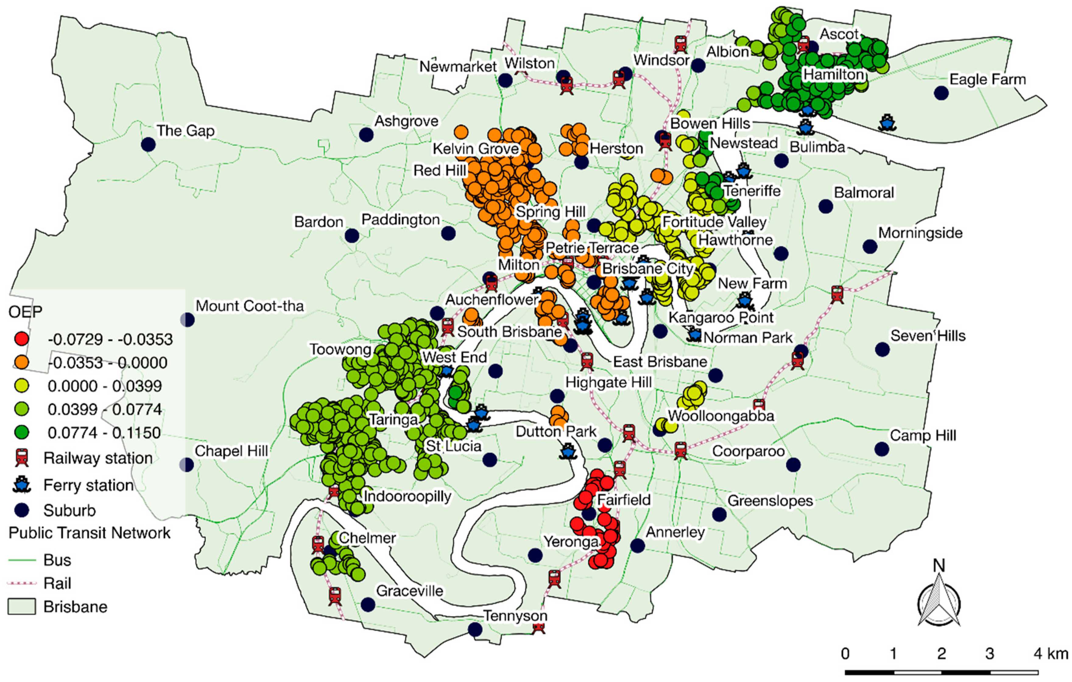
The number of morning peak-hour trips (OMP) and the number of jobs accessible by public transport within a 30-min journey during morning peak hours (JobAccess) are found to have positive impacts on property values and are statistically significant. For every 1000 trips that took place during the morning peak-hour period, a property value can be affected by a premium of $14,389 AUD, or 2.46% of the mean property value. Furthermore, the 30-min job accessibility factor is shown to be statistically significant—every 1000 jobs positively influences the property value at the rate of 0.04%, translating to a monetary value of $234 AUD. For every kilometre away from the CBD, properties in the SA1 area experience a decrease in value, on average, of 4.25%, which is equivalent to $24,859 AUD of the mean property value. Although being within 400 m to a rail station confers a premium value of $12,517 AUD (at the mean property value), being within 800 m of a ferry station does not show any significant impact on property values. The insignificance of the evening peak (OEP) coefficient can be attributed to the preference for upscale homes in residential-oriented zones. The insignificance of transfers is not surprising since the interpretation is ambiguous, being either a measure of connectivity or related to difficulty in reaching a desired destination. Likewise, the number of trips to the CBD conflates several contradictory issues, such as the premium paid for living near the CBD and the inconvenience of travelling on transit to anywhere besides the CBD from more distant suburbs where prices are low. It should be noted that, since only a day’s worth of smart card data is available in this study, it is possible that there may be a censoring issue due to this limitation.
5.2. GWR Model
In a GWR model, the spatially-varying effects of the same variable can be logically explained by spatial heterogeneity in its relationship with the dependent variable. This differs from an OLS model, which assumes that a single model fits the entire study area. Hence, depending on other attributes, whether captured or omitted, the sign and scale of the GWR coefficients can change to reflect the spatial variation of the relationship. Table 5 displays the ranges of significant parameters (p-value less than 0.05) and goodness-of-fit values of the GWR model. The GWR model outperforms the three models discussed earlier by a substantially lower AIC (−1519.62) and higher adjusted R-squared of 0.741, after the degrees of freedom are taken into account. The Moran’s I test result indicates the residuals are spatially correlated, however, with only a subtle positive effect (Moran’s I statistics of 0.0017 and p-value of 0.008). It should be noted that rectifying the spatial autocorrelation in residuals is not a direct goal of GWR.
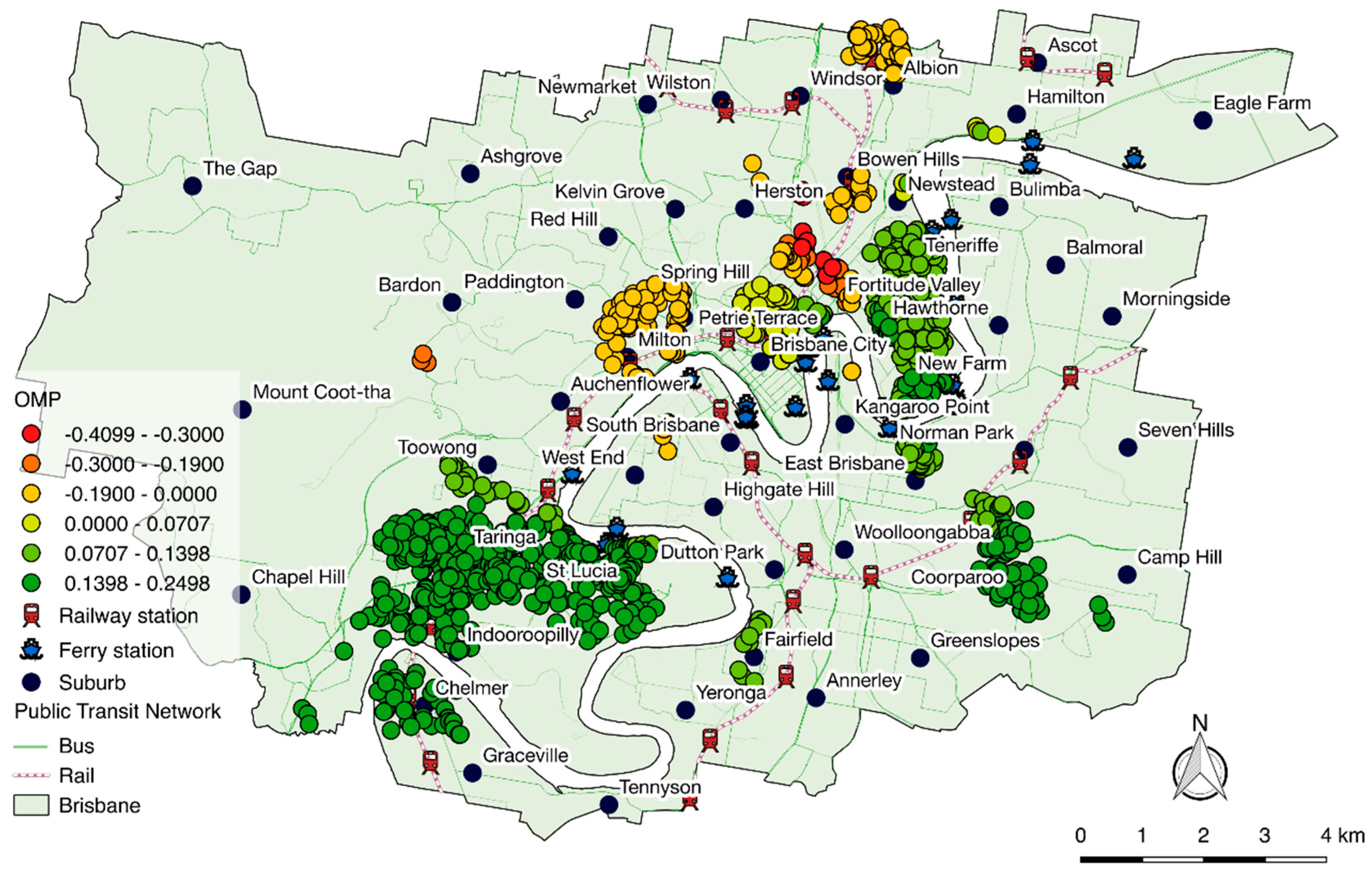
One of the many advantages of GWR is that coefficient estimations of the local model can be mapped (Figure 4 for example). However, the focus of this paper is on transit accessibility variables—OMP, EMP, NTF, CBDTrips, Bus, JobAccess—hence, only the coefficients of these variables are shown. Note that all estimations shown in the following figures are found to be statistically significant at a p-value lower than 0.05; those exceeding the p-value threshold were omitted from the figures.
It is apparent from the maps in Figure 4, Figure 5, Figure 6, Figure 7, Figure 8 and Figure 9 that spatial variation exists in the estimates of the transit accessibility variables. In Figure 4, the effect of morning peak trips, OMP, to property price varies from positive to negative across suburbs in contrast to the average effect found in the global estimate for the OLS model in Table 4. The majority of properties are associated with a positive effect, with the premiums ranging from a 7% to 25% increase per 1000 morning trips, which is aligned with its global interpretation. It is also positive in the most attractive destination of the city, the CBD, where many transit commuters transfer. In south-western suburbs, low to medium density residential housing dominates and OMP positively influences property values. Areas near train stations are affected by the number of morning trips as they have a high level of accessibility to train stations where many bus passengers come to transfer, which is in accordance with other literature [65]. It should be noted that both the south-western suburbs and the eastern suburbs, where a positive association between high property values and number of morning trips exist, have many young workers and students, which are the main demographics of public transport users in Brisbane [66]. However, for those properties in the mixed-use areas around Paddington or Milton stations and in Fortitude Valley, Brisbane’s nightlife suburb, the number of morning trips has negative effects on property values.
Evening traffic is constituted mainly from non-work-related trips—including shopping, personal business, recreation, etc.—and returning home trips, as supported by the How Queensland Travels report [45]. In Figure 5, the effect of the number of evening trips is shown. Most properties are affected by the number of evening trips occurring around them. Transit-accessible properties located near recreational areas with mixed-use in Chelmer, Taringa, and Toowong stations are positively affected by the number of departing trips in evening peak hours, up to 12% or $64,339 AUD of the average property value for every 1000 trips. Hamilton, a suburb close to Brisbane Airport to the north-east of the CBD with low-medium residential buildings next to an industrial area just to the south of the airport, also experiences premiums. It is also well connected to public transport networks via a ferry station and two train stations. Similar results are present for suburbs with nightlife (Fortitude Valley), commercial, and recreational (Newstead) activities. The number of evening trips is the highest near job centres (evening commuters) or commercial and recreational activities (non-commute destinations)—areas with these attributes show positive relationship between land values and evening transit use. Interestingly, properties near the CBD show a negative relationship between the OEP variable and price. This suggests that congestion caused by the evening activities maybe a disincentivizing factor that pushes people away from living near the CBD area. Thus, it is reflected in decreased property values.
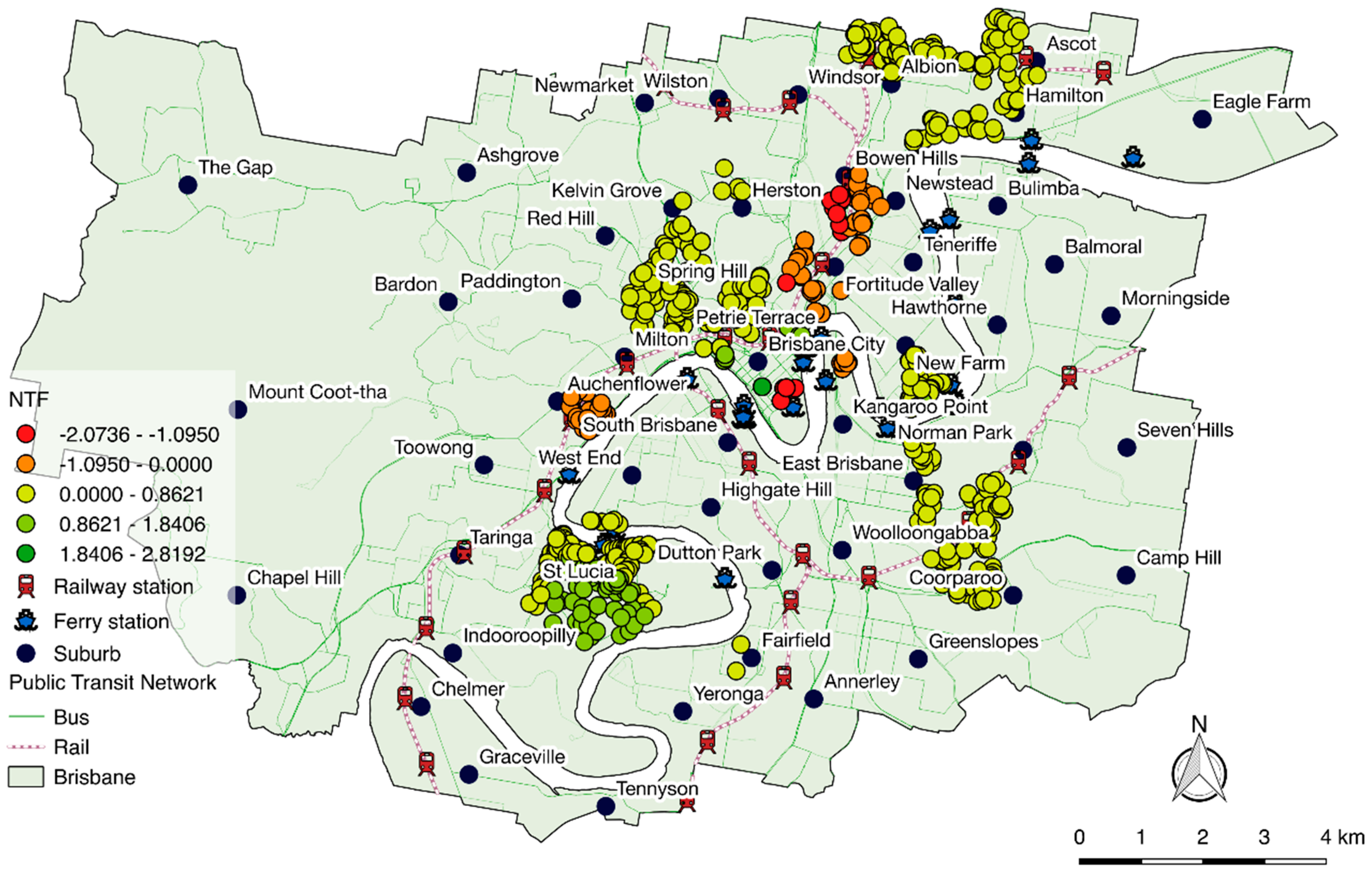
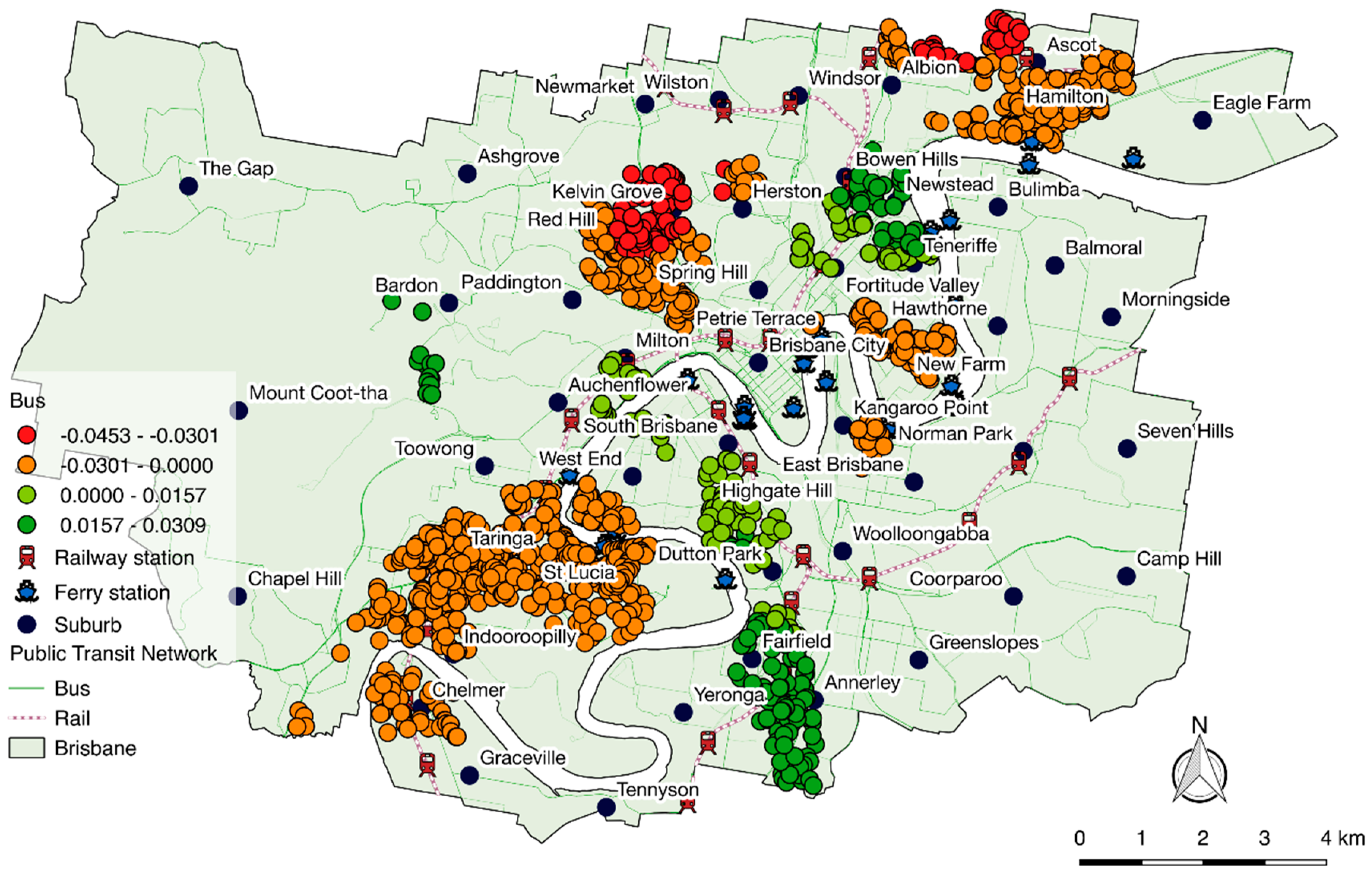
In Figure 6, differences in property values in some areas can be seen to be associated with the fraction of trips having at least one transfer. The results for the transfer variable confirm the expected sign, with an average increase of 8% in property values for every 10% change in the transfer fraction variable. This can be translated into the dollar amount of approximately up to $46,792 AUD of the mean property value. Clusters of negative associations near train stations indicate that transfers are not necessary in these highly-valued locations. Trips which consist of one or more transfers could indicate trip chaining as it is a very common travel behaviour for a trip to have more than one purpose [67]. As discussed above, the proportion of trips with at least one transfer is ambiguous for accessibility. Several suburbs without train lines obtain premium values from the proportion of local departing passengers who made at least one transfer in their journeys. In these areas, feeder buses serve to connect residents to the rail network. While it would be interesting to see the effect of feeder buses on property values, it is difficult to distinguish between regular bus line and feeder buses from this data.
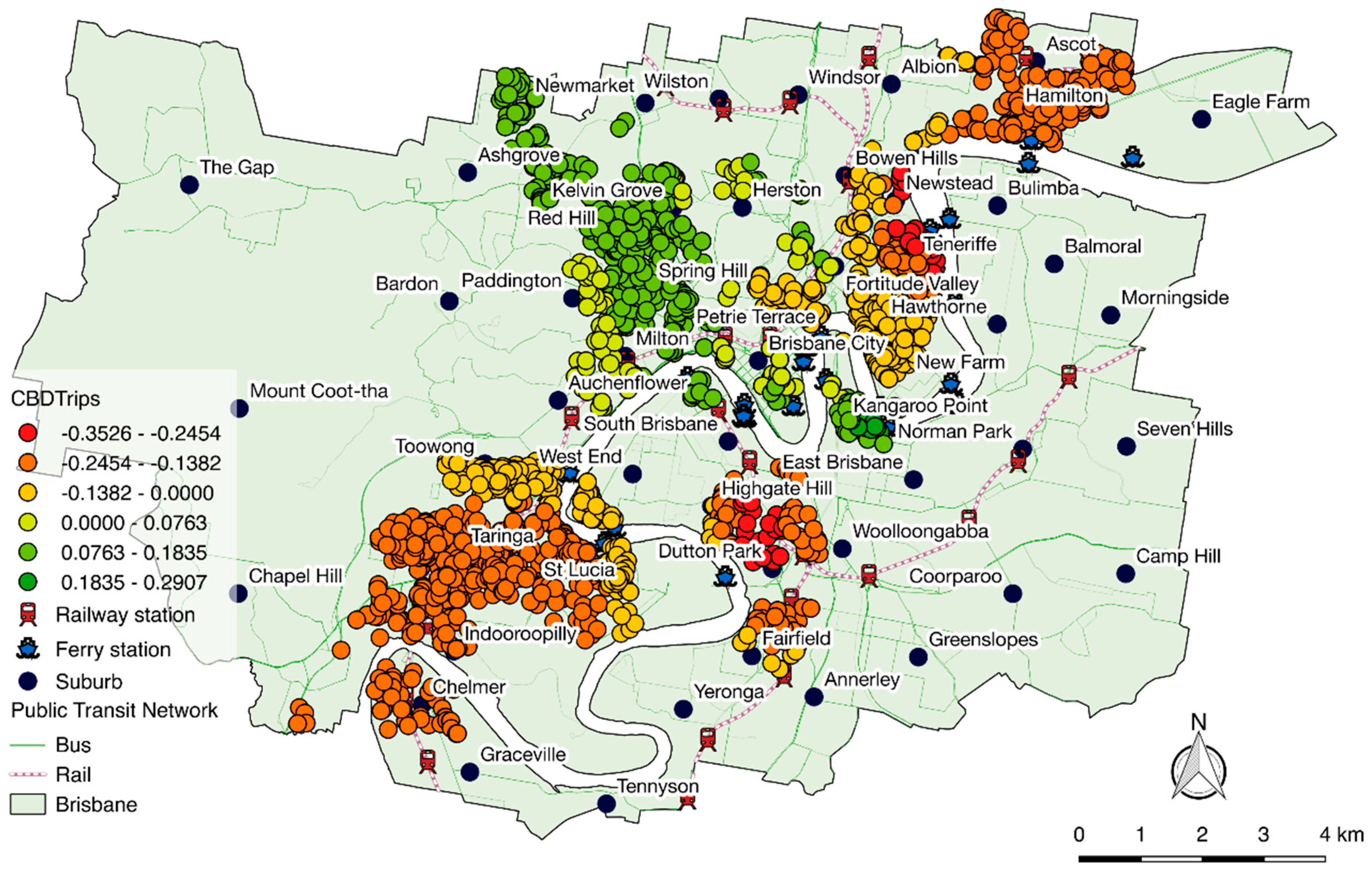
In Figure 7, the relationship between the number of CBD trips via public transport and property values is shown. This variable can be thought of as a proxy to infer the degree of connectivity of a zone to the CBD and access to its employment opportunities and amenities. Negative associations between the number of trips headed to CBD and property values are observed for south and south-western suburbs, which reflects the importance of the University of Queensland, St. Lucia, as an employment and activity centre outside the CBD. Positive influences on property values due to the number of CBD trips occur mostly in the suburbs to the north-west of the CBD, where only bus services are available to public transport users. Perhaps this highlights that those areas that do not have access to the main rail network value CBD accessibility more than those well-off areas.
Figure 8 shows the number of bus stops within 400 m to the property and their impact on the value of properties across Brisbane. In total, 87% of public transport users in Brisbane will walk or cycle to the bus stop [45]. While the global average effect of the variable shows a significant and positive relationship with the value of nearby properties which are conveniently located within a suitable walking or cycling range of bus transit nodes, the local results from GWR reveal a spatially mixed effect. Properties along the south-west rail line experience decreased property values, with the lowest at −4.5%, whereas properties on the south bank of the river experience premium values of up to 3% associated with more bus stops in the neighbourhood. Intuitively, a property that has access to many bus stops has positive effects (e.g., accessibility, attractiveness) and negative effects (e.g., noise, traffic-related air pollution, crime). Hence, this variable may need to be further investigated for its impacts affecting property values.
Finally, in Figure 9, job accessibility is visualized. The number of jobs accessible by public transport services within 30 min of travel time shows a positive and significant impact on property values. A clear pattern can be observed in the figure, where most properties close to the CBD have high property values. The weak negative relationship observed in Newstead is driven, perhaps, by either low job accessibility or low property values. Living close to major bus routes, rail stations, and ferry stations affects the number of jobs accessible by public transport. Hence, those properties in close proximity to the major transport routes and the CBD show premiums in their values ranging from 0.1% to 0.42% per 1000 accessible jobs or $585 to $2457 in premium, at the mean property value.
6. Discussion and Conclusions
Our results have shown that by introducing public transport ridership as independent variables, from smart card data, the property hedonic pricing models have improved in their explanatory power. Public transport use data reveals the importance of ridership and performance of the nearby transit nodes to the premium associated with residential property prices while controlling for the main determinants of property prices. The traditional way of identifying public transport accessibility as proximity to transit stop infrastructure does not reveal the mechanism by which service provision and traveller behaviour impact the value of properties. To better examine the relationship between property prices and transit accessibility, we used spatial regression models from the literature [68,69,70]. As expected, the OLS model was outperformed by the spatial models, which capture spatial heterogeneity and spatial dependence in the data.
The results of the GWR model, the best fitting model, show that the effects of each independent variable differ spatially in their magnitude and significance level. The number of morning trips and the number of evening trips show interesting results which, on average, confirm what has been found by other studies. The effect of the number of morning trips is mostly positive where accessibility is high, generally along the rail network, as also found by other studies [16,24]. A similar pattern was also observed in the number of evening peak trips except in and around the CBD, where a negative relationship with property values exists. This may be due to the possible nuisances of living in the city’s core, such as noise pollution [71] and congestion [72]. The aforementioned annoyances are also true for properties located near transit hubs. However, a study by Wang et al. [73] shows that in Cardiff, Wales, the number of bus stops within walking distance to a property has a positive correlation with the property price at sale. It is also empirically evident that properties of higher market prices benefit more from this than their counterparts. Wang also suggests that by forming land value tax based on this finding, policy makers can ‘ensure a more just distribution of the economic welfare yielded by public investment’. Our findings support what Wang et al. reported regarding the positive value of bus stops within 400 m. The proportion of transfers shows mostly positive values for properties without rail and ferry stations nearby, which is hard to interpret due to the transfer rate either being a measure of connectivity or related to the difficulty in reaching a desired destination. Future research may consider developing alternative indicators which could capture the two effects independently from one another. Lastly, high access to employment opportunities positively influences property values, which is in accordance with many related studies [72,74]. This is also in line with the existing literature on housing [75,76,77], where job accessibility is frequently found to be an important factor when households determine their housing location choice.
Rogers [78] found that people who live in neighbourhoods that are far from employment opportunities have a higher rate of unemployment due to low accessibility to jobs and also spend more time to secure a job again. This finding suggests that people should value access to job opportunities and therefore be willing to pay more for properties in neighbourhoods which have high access to employment. A better understanding of the mechanisms by which transit service provision impacts property values indicates that policy makers are justified in capturing the added value in order to fund growth in transit in similar neighbourhoods. Rashidi et al. [79] found that a household relocation may be followed by a job relocation for a household member and this could be due to the increase in travel time which precipitated the change of job. This agrees with this paper’s finding that the employment opportunities provided by the available public transport services are positively correlated with property values. Collectively, this evidence supports the adoption of alternative transit-funding mechanisms, such as value capture. The detailed transit accessibility measures available from emerging data sources, like the go card, support a fairer, evidenced-based implementation of value capture tools [80].
Another important finding was that reliability-related variables were not significant in determining housing prices. While reliability indicators have been found to affect short-term decisions, such as mode and route choice decisions [81,82], they seem not to be critical when it comes to residential location decisions. In other words, people consider their expected travel time to opportunities when they buy a house, but, possibly because buyers do not have information about the travel time distribution at the time of purchase, they do not value reliability. To date, no other research has examined the relationship between transit user behaviour and property prices, and reliability may emerge as a valued property attribute when the baseline of transit use data is longer.
Finally, there are some limitations that should be noted in this study. First, the relationship between property values and accessibility has a two-way interaction, where changes in each can be described as causing the other. Given the available cross-sectional data, the study could only explore the correlation between property values and accessibility. However, to be able to explore the causality and time priority of one over the other one would be advantageous for policy making and planning, see Mulley and Tsai [34] for example. Second, due to the limited smart card data available to be used in this study, the daily variability and seasonality effects of the smart card data could not be controlled. Hence, with a larger set of data, the effects of these accessibility variables could have been more explicit. Despite this limitation, this study attempted to demonstrate the value of resident-oriented public transit accessibility, which could potentially assist planners and policy makers to realise the value of public transport utilization on housing market dynamics. Lastly, another possible improvement to the study is to utilize a non-Euclidean distance metric to better capture the complexity of the transport network, as Lu et al. [37] has shown that this can improve the model fit and provide better insights into the nature of spatially varying relationships within their property price data.
Author Contributions
Conceptualization, T.H.R.; Formal analysis, A.S.; Methodology, A.S., T.H.R. and E.M.; Resources, T.H.R.; Supervision, T.H.R. and E.M.; Visualization, A.S.; Writing—original draft, A.S.; Writing—review & editing, T.H.R. and E.M.
Funding
Australian Research Council: DE170101346.
Conflicts of Interest
The authors declare no conflict of interest.
Appendix A

Table A1.
OLS model with the travel time variation indicator and the delay indicator.
| Variables | Estimate | t-Value | VIF |
|---|---|---|---|
| Beds | 0.1580 *** | 30.119 | 2.814 |
| Baths | 0.1850 *** | 29.452 | 1.586 |
| Car | 0.0313 *** | 7.079 | 1.315 |
| Unit | −0.2830 *** | −27.997 | 2.114 |
| Income | 1.0900 *** | 20.432 | 2.236 |
| Unemp | 0.8120 *** | 6.292 | 1.943 |
| Age | 0.7520 *** | 12.373 | 1.582 |
| Migration | 0.2280 *** | 4.652 | 2.409 |
| PopDen | 0.0011. | 1.586 | 1.623 |
| CBD | −0.0407 *** | −15.524 | 2.059 |
| OMP | 0.0315 *** | 3.923 | 4.292 |
| OEP | −0.0052 *** | −7.047 | 4.434 |
| NTF | 0.0913 * | 1.666 | 2.009 |
| CBDTrips | −0.0131 ** | −1.965 | 2.193 |
| SdTT | −0.0017 | −0.998 | 1.598 |
| Delay | −0.0146 | −0.604 | 1.345 |
| JobAccess | 0.0004 ** | 2.602 | 1.639 |
| Bus | 0.0016 * | 1.698 | 3.001 |
| Rail400 | 0.0262 *** | 2.752 | 1.358 |
| Ferry800 | 0.0204 ** | 2.154 | 2.083 |
| Intercept | 12.6000 *** | 372.647 | |
| Observations | 5406 | ||
| Adjusted R2 | 0.6879 | ||
| AIC | −426.9351 |
Table A2.
Variance inflated factors.
| Variable | VIF |
|---|---|
| Beds | 2.813 |
| Baths | 1.586 |
| Cars | 1.314 |
| Unit | 2.111 |
| Income | 2.233 |
| Unemp | 1.916 |
| Age | 1.579 |
| Migration | 2.385 |
| PopDen | 1.621 |
| CBD | 1.910 |
| OMP | 4.229 |
| OEP | 4.028 |
| NTF | 1.881 |
| CBDTrips | 2.181 |
| JobAccess | 1.634 |
| Bus | 2.854 |
| Rail400 | 1.330 |
| Ferry800 | 2.079 |
References
- Grengs, J. Does public transit counteract the segregation of carless households? Transp. Res. Rec. J. Transp. Res. Board 2001, 1753, 3–10. [Google Scholar] [CrossRef]
- Hensher, D.A.; Stopher, P.; Bullock, P. Service quality—Developing a service quality index in the provision of commercial bus contracts. Transp. Res. Part A Policy Pract. 2003, 37, 499–517. [Google Scholar] [CrossRef]
- Jia, W.; Wachs, M. Parking Requirements and Housing Affordability: A Case Study of San Francisco. Transp. Res. Rec. J. Transp. Res. Board 1999, 156–160. [Google Scholar] [CrossRef]
- Bamberg, S.; Hunecke, M.; Blöbaum, A. Social context, personal norms and the use of public transportation: Two field studies. J. Environ. Psychol. 2007, 27, 190–203. [Google Scholar] [CrossRef]
- Baslington, H. Travel Socialization: A Social Theory of Travel Mode Behavior. Int. J. Sustain. Transp. 2008, 2, 91–114. [Google Scholar] [CrossRef]
- Haustein, S.; Klöckner, C.A.; Blöbaum, A. Car use of young adults: The role of travel socialization. Transp. Res. Part F Traffic Psychol. Behav. 2009, 12, 168–178. [Google Scholar] [CrossRef]
- Cao, X.; Hough, J.A. Hedonic Value of Transit Accessibility: An Empirical Analysis in a Small Urban Area. J. Transp. Res. Forum 2007, 47, 171–183. [Google Scholar] [CrossRef]
- Cervero, R.; Landis, J. Assessing the impacts of urban rail transit on local real estate markets using quasi-experimental comparisons. Transp. Res. Part A Policy Pract. 1993, 27, 13–22. [Google Scholar] [CrossRef]
- Debrezion, G.; Pels, E.; Rietveld, P. The impact of railway stations on residential and commercial property value: A meta-analysis. J. Real Estate Financ. Econ. 2007, 35, 161–180. [Google Scholar] [CrossRef]
- Dubé, J.; Thériault, M.; Des Rosiers, F. Commuter rail accessibility and house values: The case of the Montreal South Shore, Canada, 1992-2009. Transp. Res. Part A Policy Pract. 2013, 54, 49–66. [Google Scholar] [CrossRef]
- Smith, V.K.; Huang, J.-C. Can markets value air quality? A meta-analysis of hedonic property value models. J. Political Econ. 1995, 103, 209–227. [Google Scholar] [CrossRef]
- Mulley, C.; Ma, L.; Clifton, G.; Yen, B.; Burke, M. Residential property value impacts of proximity to transport infrastructure: An investigation of bus rapid transit and heavy rail networks in Brisbane, Australia. J. Transp. Geogr. 2016, 54, 41–52. [Google Scholar] [CrossRef]
- Levinson, H.; Zimmerman, S.; Clinger, J.; Rutherford, G.S. Bus Rapid Transit: An Overview. J. Public Transp. 2002, 5, 1–30. [Google Scholar] [CrossRef]
- Lindquist, K.; Wendt, M.; Holbrooks, J. Transit Farebox Recovery and US and International Transit Subsidization: Synthesis; Washington State Department of Transportation: Washington, DC, USA, 2009.
- Wei, M.; Liu, Y.; Sigler, T.J. An Exploratory Analysis of Brisbane’s Commuter Travel Patterns Using Smart Card Data. In Proceedings of the State of Australian Cities Research Network; State of Australian Cities National Conference, Gold Coast, Australia, 9–11 December 2015. [Google Scholar]
- Chalermpong, S. Rail Transit and Residential Land Use in Developing Countries: Hedonic Study of Residential Property Prices in Bangkok, Thailand. Transp. Res. Rec. J. Transp. Res. Board 2007, 2038, 111–119. [Google Scholar] [CrossRef]
- Geoghegan, J.; Wainger, L.A.; Bockstael, N.E. Spatial landscape indices in a hedonic framework: An ecological economics analysis using GIS. Ecol. Econ. 1997, 23, 251–264. [Google Scholar] [CrossRef]
- Heikkila, E.; Gordon, P.; Kim, J.I.; Peiser, R.B.; Richardson, H.W.; Dale-Johnson, D. What happened to the CBD-distance gradient: Land values in a policentric city. Environ. Plan. A 1989, 21, 221–232. [Google Scholar] [CrossRef]
- Gibbons, S.; Machin, S. Valuing School Quality, Better Transport and Lower Crime: Evidence from House Prices. Oxf. Rev. Econ. Policy 2008, 24, 99–119. [Google Scholar] [CrossRef]
- Eboli, L.; Forciniti, C.; Mazzulla, G. Service coverage factors affecting bus transit system availability. Procedia-Soc. Behav. Sci. 2014, 111, 984–993. [Google Scholar] [CrossRef]
- Von Thunen, J.H. Die isolierte Staat in Beziehung auf Landwirtshaft und Nationalökonomie; Wartenberg, C.M., English Translator 1966; Hall, P.G., Ed.; Pergamon Press: New York, NY, USA, 1826. [Google Scholar]
- Alonso, W. Location and Land Use: Toward a General Theory of Land Rent; Harvard University Press: Cambridge, MA, USA, 1964; Volume 13, ISBN 0674537009. [Google Scholar]
- Munoz-Raskin, R. Walking accessibility to bus rapid transit: Does it affect property values the case of Bogota, Colombia. Transp. Policy 2010, 17, 72–84. [Google Scholar] [CrossRef]
- Parsons Brinckerhoff. The Effect of Rail Transit on Property Values: A Summary of Studies; NEORail: Cleveland, OH, USA, 2001. [Google Scholar]
- Read, P.; Heywood, C. The Effects of Accessibility Gains on Residential Property Values in Urban Areas: The Example of the T2 Tramway in the Hauts-de-Seine Department, France; Leeuwenhorst: Noordwijkerhout, The Netherlands, 2007. [Google Scholar]
- Tsai, C.-H.; Mulley, C.; Burke, M.; Yen, B. Exploring property value effects of ferry terminals: Evidence from Brisbane, Australia. J. Transp. Land Use 2015, 10. [Google Scholar] [CrossRef]
- Lancaster, K.J. A New Approach to Consumer Theory. J. Political Econ. 1966, 74, 132–157. [Google Scholar] [CrossRef]
- Rosen, S. Hedonic Prices and Implicit Markets: Product Differentiation in Pure Competition. J. Polit. Econ. 1974, 82, 34–55. [Google Scholar] [CrossRef] [Green Version]
- Chau, K.W.; Chin, T.L. A Critical Review of Literature on the Hedonic Price Model. Int. J. Hous. Sci. Its Appl. 2003, 2, 145–165. [Google Scholar]
- Bae, C.-H.C.; Jun, M.-J.; Park, H. The impact of Seoul’s subway Line 5 on residential property values. Transp. Policy 2003, 10, 85–94. [Google Scholar] [CrossRef]
- Bowes, D.R.; Ihlanfeldt, K.R. Identifying the Impacts of Rail Transit Stations on Residential Property Values. J. Urban Econ. 2001, 50, 1–25. [Google Scholar] [CrossRef]
- Huang, W. The Effects of Transportation Infrastructure on Nearby Property Values: A Review of Literature. No. Working Paper 620. 1994. Available online: http://citeseerx.ist.psu.edu/viewdoc/summary?doi=10.1.1.502.131 (accessed on 28 April 2019).
- Iacono, M.; Levinson, D. Location, Regional Accessibility, and Price Effects: Evidence from Home Sales in Hennepin County, Minnesota. Transp. Res. Rec. J. Transp. Res. Board 2011, 87–94. [Google Scholar] [CrossRef]
- Mulley, C.; Tsai, C. When and how much does new transport infrastructure add to property values? Evidence from the bus rapid transit system in Sydney, Australia. Transp. Policy 2016, 51, 15–23. [Google Scholar] [CrossRef]
- Cellmer, R. The Use of the Geographically Weighted Regression for the Real Estate Market Analysis. Folia Oeconomica Stetin. 2012, 11, 19–32. [Google Scholar] [CrossRef]
- Du, H.; Mulley, C. Understanding spatial variations in the impact of accessibility on land value using geographically weighted regression. J. Transp. Land Use 2012, 5, 46–59. [Google Scholar]
- Lu, B.; Charlton, M.; Fotheringham, A.S. Geographically Weighted Regression using a non-Euclidean distance metric with a study on London house price data. Procedia Environ. Sci. 2011, 7, 92–97. [Google Scholar] [CrossRef]
- Páez, A.; Scott, D.M. Spatial Statistics for Urban Analysis: A Review of Techniques with Examples. GeoJournal 2004, 61, 53–67. [Google Scholar] [CrossRef]
- Bagchi, M.; White, P.R. The potential of public transport smart card data. Transp. Policy 2005, 12, 464–474. [Google Scholar] [CrossRef]
- Agard, B.; Morency, C.; Trépanier, M. Mining public transport user behaviour from smart card data. IFAC Proc. 2006, 39, 399–404. [Google Scholar] [CrossRef]
- Morency, C.; Trépanier, M.; Agard, B. Measuring transit use variability with smart-card data. Transp. Policy 2007, 14, 193–203. [Google Scholar] [CrossRef] [Green Version]
- Devillaine, F.; Munizaga, M.; Trépanier, M. Detection of Activities of Public Transport Users by Analyzing Smart Card Data. Transp. Res. Rec. J. Transp. Res. Board 2012, 2276, 48–55. [Google Scholar] [CrossRef]
- Australian Bureau of Statistics Regional Population Growth, Australia, 2014–15. Available online: http://www.abs.gov.au/ausstats/[email protected]/mf/3218.0 (accessed on 9 May 2019).
- Australian Bureau of Statistics. Census of Population and Housing 2011; Australian Bureau of Statistics: Canberra, Australia, 2011.
- Department of Transport and Main roads of Queensland. How Queensland Travels—A Decade of Household Travel Surveys in Queensland; Department of Transport and Main roads of Queensland: Brisbane, Australia, 2016.
- Australian Bureau of Statistics. Australian Statistical Geography Standard: Volume 1—Main Structure and Greater Capital City Statistical Areas; Australian Bureau of Statistics: Canberra, Australia, 2011.
- Horner, M.W.; Murray, A.T. Spatial representation and scale impacts in transit service assessment. Environ. Plan. B Plan. Des. 2004, 31, 785–797. [Google Scholar] [CrossRef]
- Weinstein Agrawal, A.; Schlossberg, M.; Irvin, K. How far, by which route and why? A spatial analysis of pedestrian preference. J. Urban Des. 2008, 13, 81–98. [Google Scholar] [CrossRef]
- National Academies of Sciences, Engineering, and Medicine. Transit Capacity and Quality of Service Manual, 3rd ed.; The National Academies Press: Washington, DC, USA, 2013; ISBN 978-0-309-28344-1. [Google Scholar]
- Mazzulla, G.; Forciniti, C. Spatial association techniques for analysing trip distribution in an urban area. Eur. Transp. Res. Rev. 2012, 4, 217–233. [Google Scholar] [CrossRef] [Green Version]
- Weisbrod, G.; Vary, D.; Treyz, G. Economic Implications of Congestion. NCHRP Report #463; The National Academies of Sciences, Engineering, and Medicine: Washington, DC, USA, 2001. [Google Scholar]
- Baltagi, B.H. A Companion to Theoretical Econometrics; John Wiley & Sons, Inc.: Hoboken, NJ, USA, 2007; pp. 1–709. [Google Scholar]
- Calvo, F.; Eboli, L.; Forciniti, C.; Mazzulla, G. Factors influencing trip generation on metro system in Madrid (Spain). Transp. Res. Part D Transp. Environ. 2019, 67, 156–172. [Google Scholar] [CrossRef]
- Dziauddin, M.F.; Powe, N.; Alvanides, S. Estimating the Effects of Light Rail Transit (LRT) System on Residential Property Values Using Geographically Weighted Regression (GWR). Appl. Spat. Anal. Policy 2015, 8, 1–25. [Google Scholar] [CrossRef]
- Bivand, R.; Hauke, J.; Kossowski, T. Computing the Jacobian in Gaussian spatial autoregressive models: An illustrated comparison of available methods. Geogr. Anal. 2013, 45, 150–179. [Google Scholar] [CrossRef]
- Bivand, R.; Piras, G. Comparing Implementations of Estimation Methods for Spatial Econometrics. J. Stat. Softw. 2015, 63, 1–36. [Google Scholar] [CrossRef]
- R Core Team. R: A Language and Environment for Statistical Computing; R Foundation for Statistical Computing: Vienna, Austria, 2016. [Google Scholar]
- LeSage, J.P. An Introduction to Spatial Econometrics. Rev. D’économie Ind. 2008, 123, 19–44. [Google Scholar] [CrossRef]
- Osland, L. An Application of Spatial Econometrics in Relation to Hedonic House Price Modelling. J. Real Estate Res. 2010, 32, 289–320. [Google Scholar]
- Fotheringham, A.S.; Brunsdon, C.; Charlton, M. Geographically Weighted Regression: The Analysis of Spatially Varying Relationships; John Wiley & Sons, Ltd.: Hoboken, NJ, USA, 2003; ISBN 0471496162. [Google Scholar]
- Gollini, I.; Lu, B.; Charlton, M.; Brunsdon, C.; Harris, P. GWmodel: An R Package for Exploring Spatial Heterogeneity using Geographically Weighted Models. J. Stat. Softw. 2013, 63, 1–50. [Google Scholar] [CrossRef]
- Anselin, L.; Bera, A.K.; Florax, R.; Yoon, M.J. Simple diagnostic tests for spatial dependence. Reg. Sci. Urban Econ. 1996, 26, 77–104. [Google Scholar] [CrossRef]
- Anselin, L. Lagrange Multiplier Test Diagnostics for Spatial Dependence and Spatial Heterogeneity. Geogr. Anal. 1988, 20, 1–17. [Google Scholar] [CrossRef]
- Elhorst, J.P. Applied Spatial Econometrics: Raising the Bar. Spat. Econ. Anal. 2010, 5, 9–28. [Google Scholar] [CrossRef] [Green Version]
- Ma, X.; Zhang, J.; Ding, C.; Wang, Y. A geographically and temporally weighted regression model to explore the spatiotemporal influence of built environment on transit ridership. Comput. Environ. Urban Syst. 2018, 70, 113–124. [Google Scholar] [CrossRef]
- Australian Bureau of Statistics. Method of Travel to Work (ABS Census 2011). Table Builder. Finding Based on Use of ABS TableBuilder Data; Australian Bureau of Statistics: Canberra, Australia, 2011. Available online: https://www.abs.gov.au/websitedbs/censushome.nsf/home/tablebuilderdata2011basic?opendocument&navpos=240 (accessed on 8 May 2019).
- Wheeler, J.O. Trip purposes and urban activity linkages. Ann. Assoc. Am. Geogr. 1972, 62, 641–654. [Google Scholar] [CrossRef]
- Ibeas, Á.; Cordera, R.; dell’Olio, L.; Coppola, P.; Dominguez, A. Modelling transport and real-estate values interactions in urban systems. J. Transp. Geogr. 2012, 24, 370–382. [Google Scholar] [CrossRef] [Green Version]
- Ma, Y.; Gopal, S. Geographically Weighted Regression Models in Estimating Median Home Prices in Towns of Massachusetts Based on an Urban Sustainability Framework. Sustainability 2018, 10, 1026. [Google Scholar] [CrossRef]
- Du, H.; Mulley, C. Relationship between transport accessibility and land value: Local model approach with geographically weighted regression. Transp. Res. Rec. J. Transp. Res. Board 2006, 197–205. [Google Scholar] [CrossRef]
- Theebe, M.A.J. Planes, Trains, and Automobiles: The Impact of Traffic Noise on House Prices. J. Real Estate Financ. Econ. 2004, 28, 209–234. [Google Scholar] [CrossRef]
- Hou, Y. Traffic congestion, accessibility to employment, and housing prices: A study of single-family housing market in Los Angeles County. Urban Stud. 2017, 54, 3423–3445. [Google Scholar] [CrossRef]
- Wang, Y.; Potoglou, D.; Orford, S.; Gong, Y. Bus stop, property price and land value tax: A multilevel hedonic analysis with quantile calibration. Land Use Policy 2015, 42, 381–391. [Google Scholar] [CrossRef] [Green Version]
- Hwang, S.; Thill, J.-C. Influence of Job Accessibility on Housing Market Processes: Study of Spatial Stationarity in the Buffalo and Seattle Metropolitan Areas. In Geospatial Analysis and Modelling of Urban Structure and Dynamics; Jiang, B., Yao, X., Eds.; Springer: Dordrecht, The Netherlands, 2010; Volume 99, pp. 373–391. ISBN 978-90-481-8571-9. [Google Scholar]
- Guo, J.Y.; Bhat, C.R. Operationalizing the concept of neighborhood: Application to residential location choice analysis. J. Transp. Geogr. 2007, 15, 31–45. [Google Scholar] [CrossRef]
- Kim, J.H.; Pagliara, F.; Preston, J. The intention to move and residential location choice behaviour. Urban Stud. 2005, 42, 1621–1636. [Google Scholar] [CrossRef]
- Van Ommeren, J.; Rietveld, P.; Nijkamp, P. Job moving, residential moving, and commuting: A search perspective. J. Urban Econ. 1999, 46, 230–253. [Google Scholar] [CrossRef]
- Rogers, C.L. Job Search and Unemployment Duration: Implications for the Spatial Mismatch Hypothesis. J. Urban Econ. 1997, 42, 109–132. [Google Scholar] [CrossRef]
- Rashidi, T.H.; Mohammadian, A.K.; Koppelman, F.S. Modeling interdependencies between vehicle transaction, residential relocation and job change. Transportation 2011, 38, 909–932. [Google Scholar] [CrossRef]
- Terrill, M.; Emslie, O. What Price Value Capture? The National Academies of Sciences, Engineering, and Medicine: Melbourne, Australia, 2017; ISBN 978-0-9876121-2-0. [Google Scholar]
- Carrion, C.; Levinson, D. Value of travel time reliability: A review of current evidence. Transp. Res. Part A Policy Pract. 2012, 46, 720–741. [Google Scholar] [CrossRef]
- Li, Z.; Hensher, D.A.; Rose, J.M. Willingness to pay for travel time reliability in passenger transport: A review and some new empirical evidence. Transp. Res. Part E Logist. Transp. Rev. 2010, 46, 384–403. [Google Scholar] [CrossRef]
Figure 1.
Study area, Brisbane city.

Figure 2.
The aggregation distances of different type of stations/stops to a property.

Figure 3.
Number of jobs accessible by public transport from each zone within a 30-min journey.

Figure 4.
The spatial variability of the effect of the number of morning trips (OMP) on property values.
Figure 4.
The spatial variability of the effect of the number of morning trips (OMP) on property values.

Figure 5.
The spatial variability of the effect of the number of evening trips (OEP) on property values.
Figure 5.
The spatial variability of the effect of the number of evening trips (OEP) on property values.

Figure 6.
The spatial variability of the effect of the proportion of transfers variable (NTF) on property values.
Figure 6.
The spatial variability of the effect of the proportion of transfers variable (NTF) on property values.

Figure 7.
The spatial variability of the effect of the number of trips to the CBD (CBDTrips) on property values.
Figure 7.
The spatial variability of the effect of the number of trips to the CBD (CBDTrips) on property values.

Figure 8.
The spatial variability of the effect of bus stop count (Bus) on property values.

Figure 9.
The spatial variability of the effect of job accessibility (JobAccess) on property values.
Figure 9.
The spatial variability of the effect of job accessibility (JobAccess) on property values.

Table 1.
An example of a trip record on go card.
| Field | Data |
|---|---|
| Journey ID | 2013030309154727000985071 |
| Trip ID | 1 |
| Operator | Brisbane Transport |
| Run | 4008 |
| Route ID | 130 |
| Service ID | 8025 |
| Direction | Inbound |
| Boarding Time | 1/03/2013 5:29 |
| Alighting Time | 1/03/2013 5:46 |
| Boarding Stop | “Ridgewood Heights” Ridgewood Road [BT005863] |
| Alighting Stop | “Sunnybank” Mains Road [BT005638] |
Table 2.
Descriptive statistics.
| Variables | Description | Mean | St Dev. | Source |
|---|---|---|---|---|
| Price | Price of the property | 584,900 | 295,534 | CoreLogic |
| Beds | Number of bedrooms | 2.39 | 1.01 | CoreLogic |
| Bathrooms | Number of bathrooms | 1.65 | 0.63 | CoreLogic |
| Car | Number of car spaces | 1.14 | 0.82 | CoreLogic |
| Unit | Property’s type (house = 0, unit = 1) | 0.71 | - | CoreLogic |
| Income | Percentage of people with weekly income greater than $1500 | 22% | 9% | ABS [44] |
| Age | Percentage of people aged greater than 65 | 12% | 7% | ABS [44] |
| PopDen | Population density in the statistical area (1000 persons) | 5.54 | 6.02 | ABS [44] |
| Mobility | Percentage of household residential location changed since last year | 27% | 10% | ABS [44] |
| Unemp | Percentage of unemployed persons | 6% | 3% | ABS [44] |
| OMP | Number of trips originated during the morning peak hours (1000s of trips) | 0.84 | 0.81 | go card |
| OEP | Number of trips originated during the evening peak hours (1000s of trips) | 3.92 | 9.03 | go card |
| NTF | Proportion of transfer trips of all originated trips | 0.15 | 0.08 | go card |
| sdTT | Average travel time variability (min) | 13.79 | 2.33 | go card |
| Delay | Travel time delay during the morning peak hours (min) | 0.3 | 0.15 | go card |
| CBDTrips | Trips to CBD (1000s of trips) | 0.75 | 0.7 | go card |
| Bus | The number of bus stops within 400 m of the property | 3.63 | 5.92 | GTFS |
| Rail400 | The property is located within 400 m within to a rail station (yes = 1, no = 0) | 0.18 | - | GTFS |
| Ferry800 | The property is located within 800 m to a ferry station (yes = 1, no = 0) | 0.37 | - | GTFS |
| JobAcess | Jobs accessible within a 30-min journey by public transit services (1000s of jobs) | 21.66 | 26.55 | go card and ABS [44] |
| CBD | Network distance from the statistical zone where the property is located to the CBD (km) | 2.98 | 1.73 | Google MAP API |
Note: ‘Unit’, ‘400 m within a rail station’ and ‘800 m within a ferry station’ are dummy variables. If the property’s type is a house, then ‘Unit’ holds a value of ‘0’, otherwise ‘1’. For the latter two variables, if yes, then they hold a value of ‘1’, otherwise ‘0’.
Table 3.
Spatial dependence tests.
| Value | p-Value | |
|---|---|---|
| Lagrange Multiplier (error) | 1185.30 | <0.001 |
| Robust LM (error) | 1093.20 | <0.001 |
| Lagrange Multiplier (lag) | 95.80 | <0.001 |
| LM Robust (lag) | 3.73 | 0.053 |
Table 4.
Results of the global models.
| OLS | Spatial Lagged | Spatial Error | |||||
|---|---|---|---|---|---|---|---|
| Estimate | t Value | Estimate | t Value | Estimate | t Value | ||
| Beds | 0.1581 *** | 30.095 | 0.1577 *** | 30.262 | 0.1634 *** | 32.289 | |
| Baths | 0.1848 *** | 29.464 | 0.1803 *** | 28.896 | 0.1746 *** | 28.770 | |
| Car | 0.0311 *** | 7.036 | 0.0309 *** | 7.028 | 0.0284 *** | 6.724 | |
| Unit | −0.2829 *** | −28.058 | −0.2694 *** | −26.666 | −0.3015 *** | −29.880 | |
| Income | 1.0900 *** | 20.441 | 0.8322 *** | 13.764 | 0.8868 *** | 13.233 | |
| Unemp | 0.7888 *** | 6.156 | 0.6318 *** | 4.885 | 0.3430 ** | 2.190 | |
| Age | 0.7507 *** | 12.370 | 0.7861 *** | 13.001 | 0.7681 *** | 10.409 | |
| Mobility | 0.2265 *** | 4.637 | 0.3119 *** | 6.234 | 0.1033 * | 1.800 | |
| PopDen | 0.0011 | 1.639 | 0.0019 *** | 2.700 | 0.0027 *** | 3.560 | |
| CBD | −0.0415 *** | −16.437 | −0.0402 *** | −15.912 | −0.0425 *** | −5.310 | |
| OMP | 0.0312 *** | 3.907 | 0.0283 *** | 3.621 | 0.0246 * | 1.868 | |
| OEP | −0.0053 *** | −7.497 | −0.0039 *** | −5.366 | −0.0017 | −1.303 | |
| NTF | 0.1015 * | 1.914 | 0.0752 | 1.149 | 0.0810 | 0.989 | |
| CBDTrips | −0.0137 ** | −2.075 | −0.0034 | −0.397 | −0.0084 | −0.681 | |
| JobAceess | 0.0004 *** | 2.619 | 0.0004 ** | 2.273 | 0.0004 ** | 2.565 | |
| Bus | 0.0017 * | 1.924 | 0.0017 * | 1.809 | −0.0018 | −1.472 | |
| Rail | 0.0244 *** | 2.584 | 0.0315 *** | 3.237 | 0.0214 * | 1.784 | |
| Ferry | 0.0209 ** | 2.208 | 0.0159 * | 1.699 | 0.0021 | 0.154 | |
| Constant | 12.5900 *** | 377.905 | 9.4995 *** | 27.258 | 12.7400 *** | 264.013 | |
| Rho/lambda coefficient | 0.2355 | 0.7733 | |||||
| Observations | 5406 | 5406 | 5406 | ||||
| Adjusted R2 | 0.688 | 0.693 | 0.71 | ||||
| AIC | −428.646 | −508.741 | −812.934 | ||||
Note: Significant codes: * p < 0.1, ** p < 0.05, *** p < 0.01.
Table 5.
Result of the GWR model.
| Variable | Median | Std Dev. | Min | Max |
|---|---|---|---|---|
| Beds | 0.1739 | 0.0428 | 0.0930 | 0.2770 |
| Baths | 0.1685 | 0.0336 | 0.0496 | 0.2686 |
| Cars | 0.0390 | 0.0148 | 0.0224 | 0.0822 |
| Unit | −0.3025 | 0.0440 | −0.4003 | −0.1465 |
| Income | 0.8625 | 0.2472 | 0.3708 | 1.8925 |
| Unemp | 1.1187 | 1.1596 | −1.7343 | 3.6156 |
| Age | 0.9566 | 0.3817 | −0.6396 | 1.8730 |
| Mobility | 0.3066 | 0.6113 | −1.3640 | 0.7758 |
| PopDen | 0.0044 | 0.0093 | −0.0275 | 0.0168 |
| CBD | −0.0596 | 0.1040 | −0.3653 | 0.3879 |
| OMP | 0.1230 | 0.1516 | −0.4099 | 0.2498 |
| OEP | 0.0122 | 0.0400 | −0.0729 | 0.1150 |
| NTF | 0.4888 | 0.8018 | −2.0736 | 2.8192 |
| CBDTrips | −0.1030 | 0.1321 | −0.3526 | 0.2907 |
| JobAccess | 0.0013 | 0.0013 | −0.0021 | 0.0042 |
| Bus | −0.0157 | 0.0181 | −0.0453 | 0.0309 |
| Rail400 | 0.0765 | 0.0898 | −0.1189 | 0.5016 |
| Ferry800 | 0.0564 | 0.1005 | −0.1890 | 0.3004 |
| Constant | 12.7903 | 0.2449 | 11.8914 | 13.4316 |
| Observations | 5406 | |||
| AICc | −1289.76 | |||
| AIC | −1519.62 | |||
| Adjsuted R2 | 0.741 |
© 2019 by the authors. Licensee MDPI, Basel, Switzerland. This article is an open access article distributed under the terms and conditions of the Creative Commons Attribution (CC BY) license (http://creativecommons.org/licenses/by/4.0/).
Share and Cite
MDPI and ACS Style
Siripanich, A.; Rashidi, T.H.; Moylan, E. Interaction of Public Transport Accessibility and Residential Property Values Using Smart Card Data. Sustainability 2019, 11, 2709. https://doi.org/10.3390/su11092709
AMA Style
Siripanich A, Rashidi TH, Moylan E. Interaction of Public Transport Accessibility and Residential Property Values Using Smart Card Data. Sustainability. 2019; 11(9):2709. https://doi.org/10.3390/su11092709
Chicago/Turabian StyleSiripanich, Amarin, Taha Hossein Rashidi, and Emily Moylan. 2019. "Interaction of Public Transport Accessibility and Residential Property Values Using Smart Card Data" Sustainability 11, no. 9: 2709. https://doi.org/10.3390/su11092709
Note that from the first issue of 2016, this journal uses article numbers instead of page numbers. See further details here.