Considering Emission Treatment for Energy-Efficiency Improvement and Air Pollution Reduction in China’s Industrial Sector

1
School of Economic Management, Changzhou Vocational Institute of Mechatronic Technology, No. 26 Middle Minxin Road, Wujin District, Changzhou 213164, China
2
Department of Economics, Soochow University, 56, Kueiyang St., Sec. 1, Taipei 100, Taiwan
*
Author to whom correspondence should be addressed.
Sustainability 2018, 10(11), 4329; https://doi.org/10.3390/su10114329
Submission received: 29 September 2018
/
Revised: 15 November 2018
/
Accepted: 18 November 2018
/
Published: 21 November 2018
Abstract
:China has one of the most serious air quality conditions in the world, with the main energy consumption and air pollution emissions coming from its industrial sector. Since 2010, the Chinese government has strengthened the governance requirements for industrial sector emissions. This study uses emission treatment as a new input on the basis of past literature, and employs the dynamic SBM model to evaluate the energy and emission-reduction efficiencies of the country’s industrial sector from 2011 to 2015. The study finds that the improvement in industrial sector efficiency is not only due to the optimization of the energy consumption structure and reduction of energy intensity, but also from investing inemission treatment methods that help cut emissions as an undesirable output. The end result is a positive effect on the improvement and sustainability of energy and emission-reduction efficiencies.
1. Introduction
China is the world’s largest energy consumer and CO2 emitter; its energy consumption accounts for about one quarter [1] of the world’s total, and its CO2 emissions accounted for 28.21% [2] of the world’s total in 2016. Due to differences in resource endowments, the country energy structure is still dominated by coal, which constituted 62% [2] of the country’s total energy consumption in 2016. In addition to CO2, coal combustion emits a large amount of SO2, NOx, and PM2.5, causing air pollution problems that led to the deaths of about 1.1 million people in China in 2015 [3].
China’s industrial sector (including mining, manufacturing, and power industries) made up about one-third of its gross domestic product (GDP) in 2016, while energy consumption and CO2 accounted for two-thirds of the country’s energy consumption and CO2 emissions [2]. In 2015, the total emissions from China’s industrial sector hit 68.5 trillion cubic meters, with SO2 accounting for 83.73%, NOx accounting for 63.79%, and soot accounting for 66.59% of the country’s emissions. Therefore, the negative effects of China’s industrial sector on energy efficiency and emission treatment have received great attention from academia, the government, and the whole society.
To address air pollutant emissions, in 2010 the Chinese government issued guiding opinions, focusing on the industrial sector, and made arrangements for government emissions control during the “12th Five-Year Plan” period (2011–2015). The main contents include setting up key areas to limit high-energy consumption industries, accelerating the replacement of coal by clean energy and renewable energy, and forcing the installation of waste gas treatment equipment by enterprises in the industrial sector.
In the treatment of air pollution, the efforts made by the Chinese government have achieved results. According to analyses of National Aeronautics and Space Administration (NASA satellite data, the levels of fine particulate matter in China fell by 17% between 2010–2015 [4]. It shows that it is of great practical significance to make a more dynamic assessment of the energy and emission-reduction efficiencies of China’s industrial sector during this period, as well as clarify the sources of its performance.
The dynamic slacks-based measure (SBM) is an application of the data envelopment analysis (DEA) method. As DEA is an efficiency analysis model for multiple inputs and outputs, more research studies are applying this form of energy-efficiency assessment. Compared to most studies based on DEA models, the dynamic SBM model normally uses a capital variable as the carry-over term in between two periods. Therefore, one can interpret the carry-over (capital) variable by the dynamic SBM model for analyzing and comparing continuous changes to decision-making units (DMUs) over years.
Färe et al. [5] first applied the DEA method to the field of energy and environment, evaluating energy efficiency through the DEA method on DMUs by using labor, capital, and energy consumption as inputs, and GDP as output. With an emphasis on the greenhouse effect, some scholars have analyzed CO2 as an undesirable output item. Such studies first appeared in comparisons between Organization for Economic Co-operation and Development (OECD) countries, such as those of Zaim et al. [6], Färe et al. [7], and Zhou and Ang [8]. With China’s strong economic growth and the imbalance between regional developments, some scholars have used the DEA international comparison method for comparisons among its provinces. Hu and Wang [9] used labor, capital, and energy consumption as inputs, and GDP as an output item, to analyze the energy efficiency of 29 provinces. Since then, this method has been used to analyze China’s energy efficiency, including by: Wei [10], Chang and Hu [11], Zou [12], Li and Lin [13], and Zhou et al. [14]. In recent years, some scholars have begun to evaluate energy efficiency by adding an undesirable output, such as Choi et al. [15], Wang et al. [16], and Wang et al. [17]. Many scholars have included China’s air pollutants other than CO2 such as SO2 or PM2.5 as undesirable outputs for analysis, such as Yeh et al. [18], Wang and Feng [19], Zhang and Choi [20], and Yu and Choi [21]. The above studies are based on static analysis.
Kao [22] emphasized that dynamic analysis is necessary whenever data are available, because system efficiency is a linear combination of the period efficiencies of a dynamic system, and ignoring the dynamic nature produces overestimated efficiencies. There are some common methods that have been employed to analyze changes in energy efficiency, such as those with window analysis and the Malmquist index. For example, Sueyoshiet al. [23] applied DEA window analysis to a data set on United States(U.S.) coal-fired power plants during 1995–2007, and found that these plants have gradually paid more attention to environmental protection issues. Wang et al. [24] used the DEA window analysis technique, analyzed China’s regional total-factor energy and environmental efficiencies, and found that environmental efficiency in China slightly increased from 2000 to 2008. Wu et al. [25] used Malmquist indices to investigate the energy utilization efficiency of China’s 30 provinces, and found that the eastern region is better than the central and western regions regarding energy efficiency. Yao et al. [26] applied the meta-frontier non-radial Malmquist CO2 emission performance index to estimate the changes in China’s CO2 emission performance. Wu et al. [27] measured the regional energy and environmental performances in China by using DEA-based Malmquist indices, and found that most regions exhibited a declining trend in technical efficiency and an increasing trend in technical progress during the 11th five-year plan period (2006–2010).
Tone and Tsutsui [28] suggested that window analysis and the Malmquist index usually neglect carry-over activities between two consecutive terms, and developed dynamic DEA into a dynamic SBM within the SBM framework. Appling this method, Guo et al. [29] used energy stock as a carry-over to evaluate the inter-temporal efficiency for executive efficiency based on fossil fuel CO2 emissions in OECD countries and China. Ke [30] used capital stock as a carry-over to evaluate the energy efficiency of Asia-Pacific Economic Cooperation (APEC) member economies over 18 consecutive years.
Some scholars have focused on China’s industrial sector to explore the relationship between energy consumption structure, energy intensity, government policies, and other factors related to energy efficiency. Cole et al. [31] found that China’s industrial emissions have a positive function on both its energy use and human capital intensity, and a negative function on its productivity. Wang et al. [32] noted that energy consumption and economic growth are the long-run causes for CO2emissions, and that CO2emissions and economic growth are the long-run causes for energy consumption, indicating that China’s CO2emissions will not decrease for a long period of time, and that reducing CO2emissions may handicap China’s economic growth to some degree. Yang et al. [33] found that there is a lack of cooperation among local governments to continue reducing energy intensity, and hence complementary policies for reducing energy and carbon intensities are needed. Dong et al. [34] indicated that the industrial sector has a better reduction potential than the other sectors, and suggested that the Chinese government should consider adjusting the energy consumption structure into existing energy policies and measures in the future.
As mentioned earlier, through the intervention of the Chinese government, companies have increased their capital investment in waste gas treatment. The result showed that for the period between 2011–2015, that there was a significant rise in the number of industrial waste gas treatment facilities in China’s industrial sector. Previous studies that employed the DEA method to assess energy efficiency often used population, capital, and energy as input variables, and GDP and undesirables (such as CO2, SO2, PM2.5, etc.) as output variables. In our research, we will add the expenditure on industrial waste gas treatment facilities (i.e., Expenditure) as a new input variable and apply industrial waste gas emissions (i.e., Emission) including CO2, SO2, NOx, Soot etc., as an undesirable output variable. In the selection of models for dynamic efficiency values, we are trying to make the necessary modifications to the dynamic SBM model proposed by Tone and Tsutsui [28] that will make it suitable for analyzing data with an undesirable output. Then, we define the efficiency value as energy and emission-reduction efficiencies. Previous studies have discussed the impact of energy efficiency improvements on the optimization of the energy consumption structure and the reduction of energy intensity. The authors used the estimated efficiency results to establish treatment intensity and emission intensity as new indicators that can help evaluate whether emission treatment has a positive effect on improving energy and emission-reduction efficiencies.
The purpose of this study is to explore the case of considering the emission treatment, energy consumption structure, and energy intensity as factors in tests. Emission intensity exists as a factor that affects the dynamic change of efficiency, in order to see if there is a positive effect on whether the change in treatment intensity improves energy and emission-reduction efficiencies.
2. Methodology and Date Sources
2.1. The Modified Dynamic SBM Model
From the development of the DEA dynamic methodology, Färe et al. [35] proposed the Malmquist index (MPI) to analyze a firm’s technical change and efficiency change, but they did not analyze the impact of carry-over activities fortwo periods. Färe and Grosskopf [36] then proposed a new analysis of the dynamic impact of consecutive activities. Tone and Tsutsui [28] extended the dynamic analysis model into a slacks-based measure. Tone and Tsutsui [28] proposed the SBM (weighted slack-based measures) dynamic DEA model, in order to carry over activities as a form of connectivity.
The methodology of this study is designed based on the Tone and Tsutsui [28] assumption, and the investigation is described as follows.
Suppose there are n DMUs over t periods; each DMU has a different input and output during period t, and there is a carry-over (link) to the next period (t + 1). The input and output that are used to compute the efficiency are labeled as and , respectively. As the basis of analysis for the dynamic DEA model, we divided the carry-over activities into four kinds: (1) desirable (good), (2) undesirable (bad), (3) discretionary (free), and (4) non-discretionary (fixed).
The following is the non-oriented model:
Equation (2) is the connection equation between periods t and t + 1.
The most efficient solution is:
Since this study considers undesirable output in the dynamic SBM model, the Tone and Tsutsui [37] dynamic SBM model can be modified to include undesirable output in the dynamic SBM model. Suppose the observations make up a (J = 1…n) dimension DMU set in which the DMU under evaluation is represented by and is subject to . The input and outputthat areused to compute the efficiency are labeled as m inputs (i = 1…m) and s outputs , respectively. Let output Y be divided into (yg, yb), where yg is a desirable output, yb is an undesirable output, and is carried over from period t to period t + 1. The following is the non-oriented model:
Equation (6) is the connection equation between periods t and t + 1.
The most efficient solution is:
2.2. Variables and Carry-Over
This study uses 30 provincial administrative units in China as DMUs, the revenue from principal business (i.e., Revenue; namely the main business income of industrial enterprises) as the desirable output, and industrial waste gas emissions (i.e., Emission; including CO2, SO2, NOx, and soot) as the undesirable output. The two traditional inputs of annual average employees (i.e., Labor), and total energy consumption (i.e., Energy) are added to the coal, petroleum, natural gas, and electricity consumed together. Furthermore, the expenditure on industrial waste gas treatment facilities (i.e., Expenditure) is added as the input, and mainly refers to the annual operating cost of waste gas treatment equipment, such as desulfurization, denitrification, and dust removal equipment. Capital stock is used as the carry-over in periods t and t+1 to assess the efficiency of energy and emissions management in China’s industrial sector. Data from 2011 to 2015are collected from the Industry Statistical Yearbook of China [37,38,39,40,41], Energy Statistical Yearbook of China [42,43,44,45,46], and Statistical Yearbooks on the Environment of China [47,48,49,50,51].
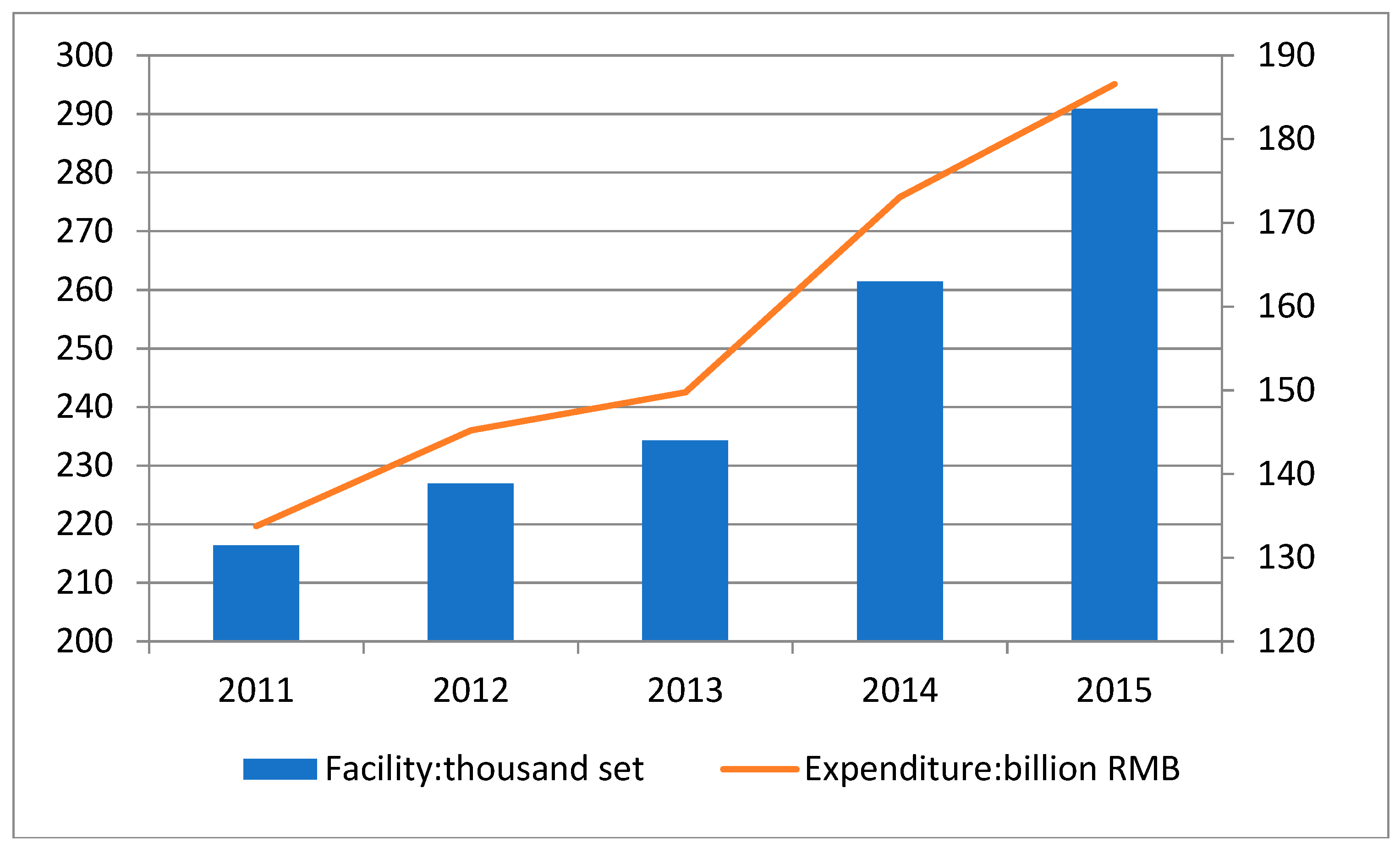
Under the guiding opinions issued by the Chinese government in 2010 in the 12th Five-Year Plan (2011–2015), which were intended to limit the emissions of high-energy industries, it is mandatory for them to install waste gas treatment machinery, including desulfurization, denitrification, and de-dusting equipment. This study found that during the five years that the number of industrial waste gas treatment facilities (i.e., Facilities) in China’s industrial sector increased significantly, the expenditure of industrial waste gas treatment facilities (i.e., Expenditure) also presented a significant increase. Figure 2 shows the trends of facility and expenditure from 2011 to 2015.
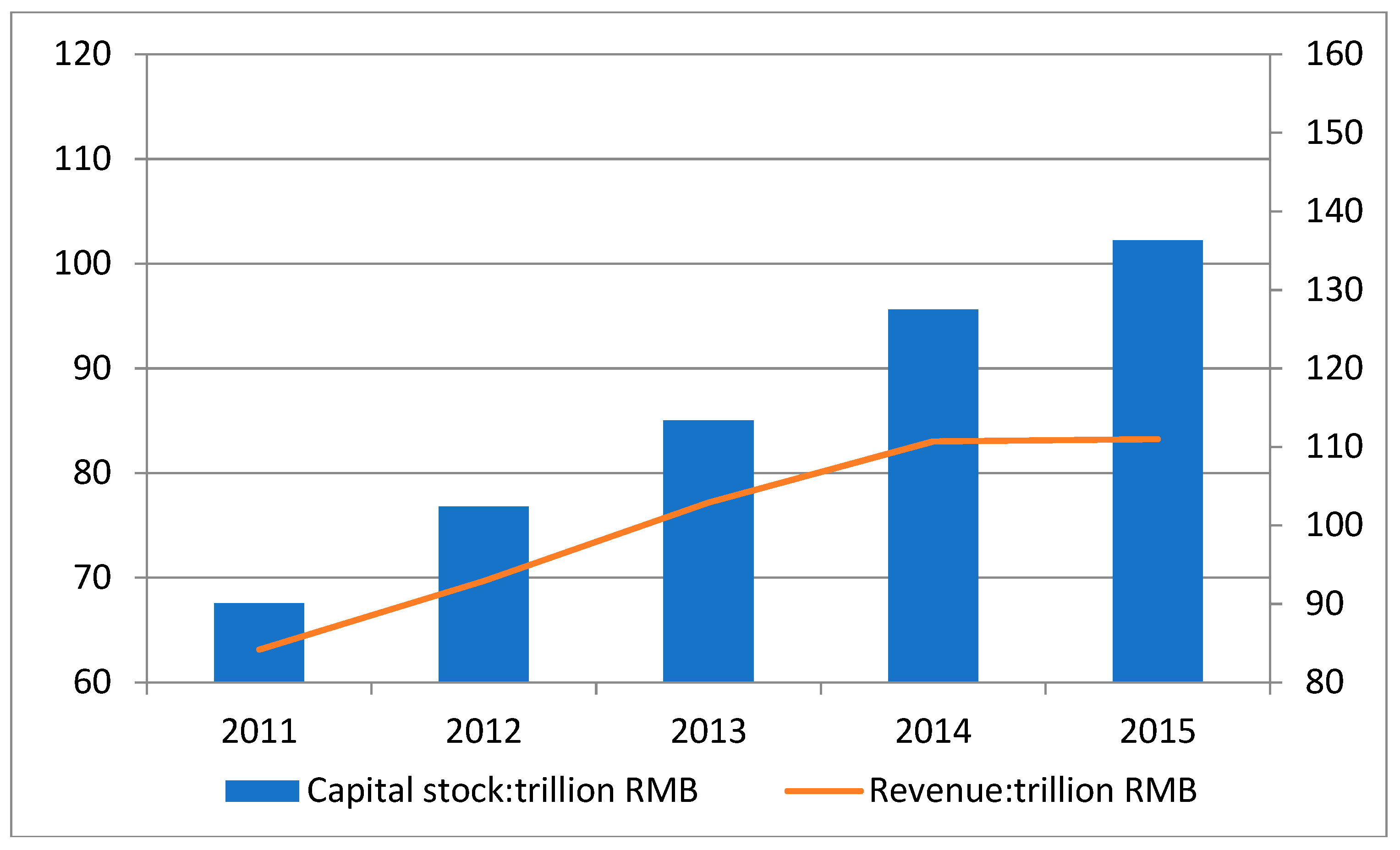
The cost of industrial waste gas treatment facilities invested by industrial enterprises is included in the capital stock. This study also investigates the relationship between capital stock and revenue from the principal business (i.e., Revenue), as well the trend during these five years. Figure 3 shows the trends of capital stock and revenue from 2011–2015.
It shows that the growth in capital stock during 2010–2015 was higher than the growth rate of the main business, especially in 2014–2015. Figure 2 illustrates a distinct increase in the input of industrial waste gas treatment facilities for 2014–2015. Thus, it easy to see that higher capital stock includes a portion that increases desirable output (Revenue) and a portion that reduces undesirable output. The undesirable output of energy consumption in the industrial sector is mainly waste gas.
3. Empirical Study
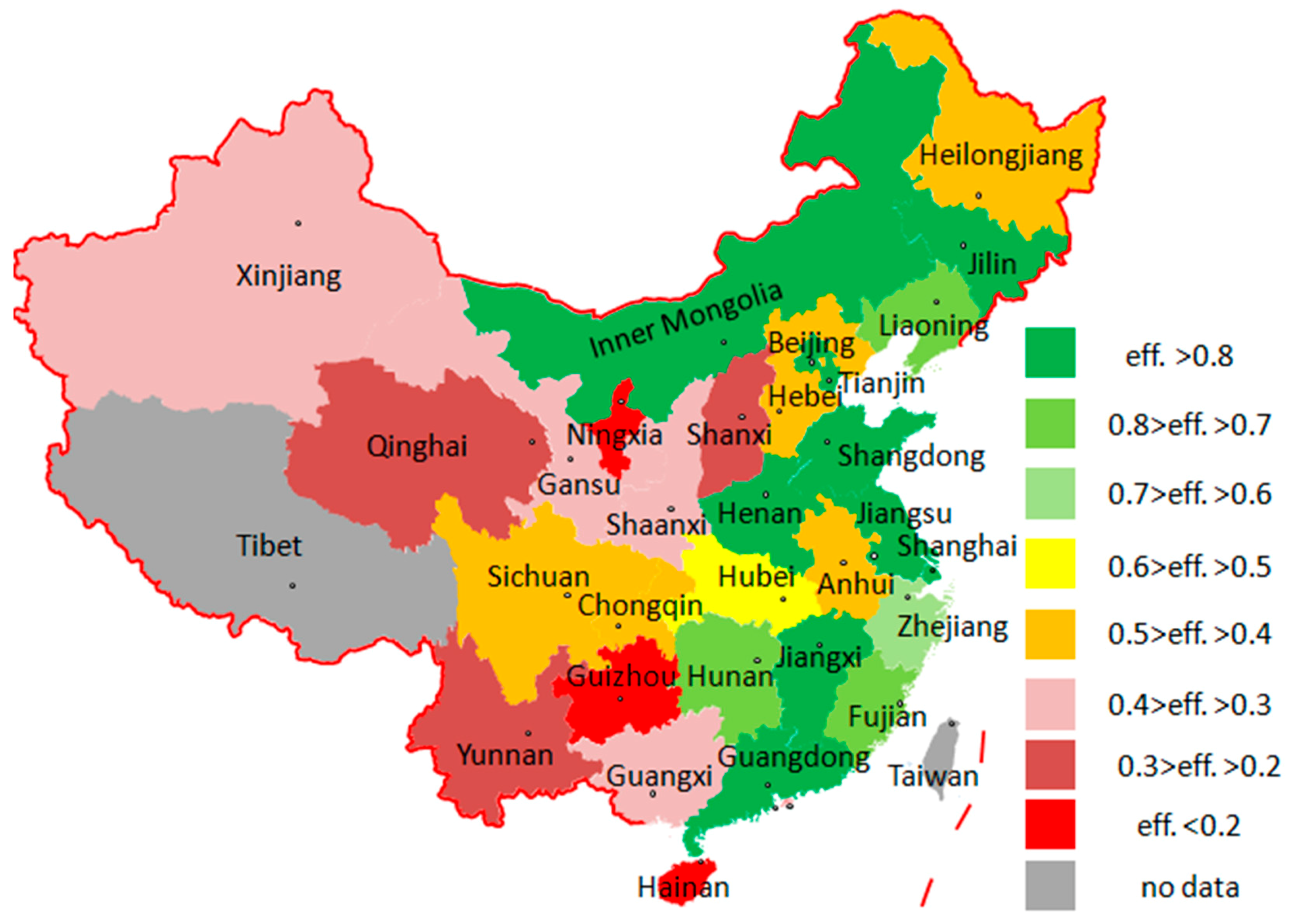
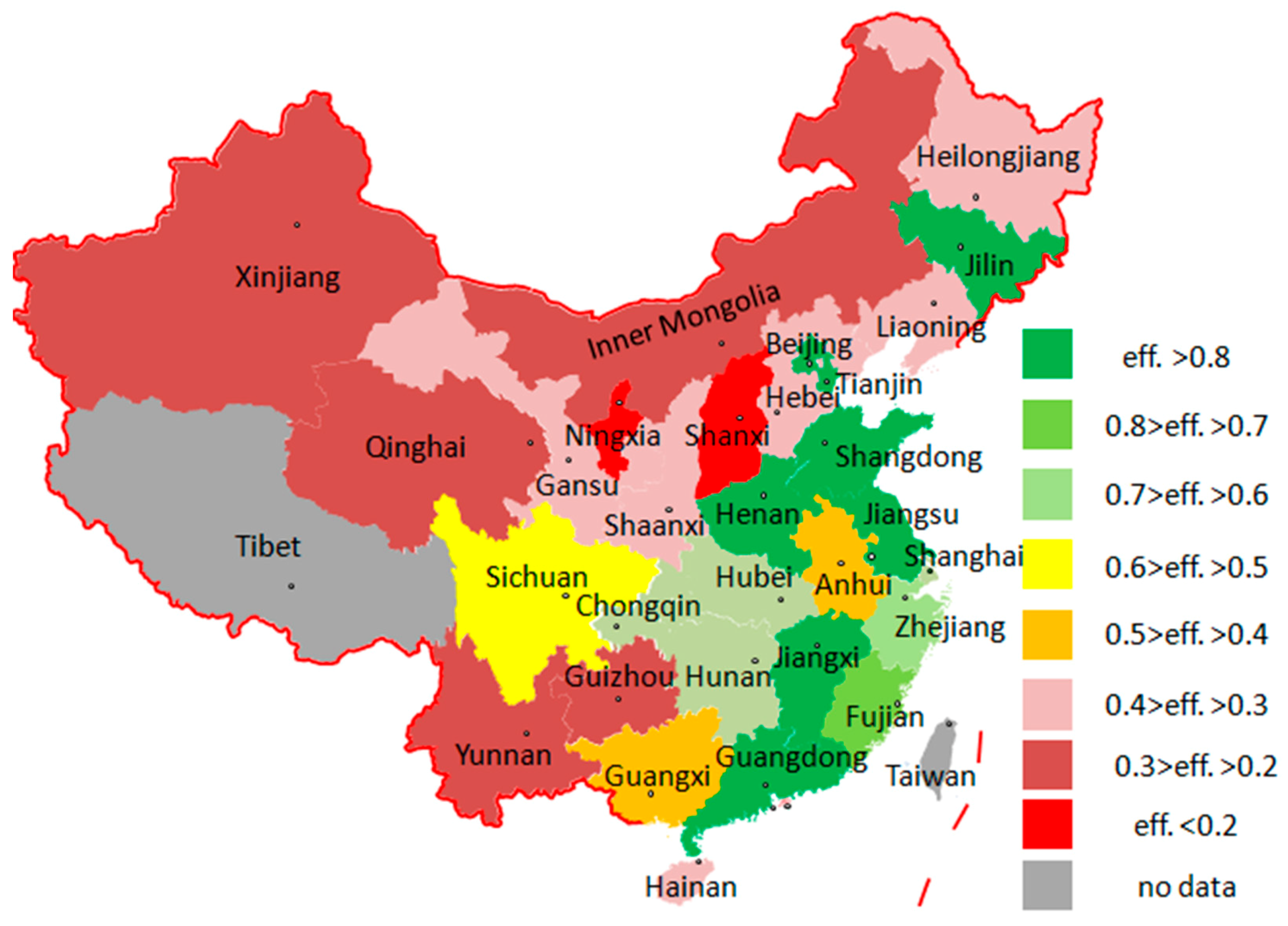
Based on the modified dynamic SBM model (8), this study estimate the energy and emission-reduction efficiency values of the industrial sectors in 30 provinces of China. Table 2 reports the results of the estimation. Figure 4 and Figure 5 compare the values of 2011 and 2015, and allow us to visually see the changes in values over the past five years. Table 2 shows that there are large differences in the efficiency values of the DMUs in different provinces, and divides the DMUs into different groups based on their values and changes over the five years.
These figures show the DMUs that have maintained a high level of energy and emission-reduction efficiency values over the five years, including Beijing, Guangdong, Jiangsu, Jiangxi, Jilin, Shandong, Shanghai, and Tianjin. Seven of the values of these eight DMUs (excluding Shanghai) are one during the five years; Shanghai fell in 2015, but its average value is 0.949. Among the 30 DMUs, only these eight DMUs’ values were greater than 0.8. This group of eight DMUs can be marked as H (High efficiency). For this group, most of them are located in eastern coastal areas with more developed economies, except Jiangxi and Jilin.
Second, it indicates the DMUs that had low energy and emission-reduction efficiency values within the five years and no growth trends; these included Gansu, Hebei, Ningxia, Qinghai, Shaanxi, Shanxi, Xinjiang, and Yunnan. These eight DMUs’ values were all less than 0.4. Although the values for Guizhou and Hainan are less than 0.4, their efficiency values show a significant upward trend, and treat these two DMUs separately. This group of eight DMUs can be marked as L (Low efficiency).
Third, it shows the DMUs that had a significant increase in energy and emission-reduction efficiency values over the past five years, including Chongqing, Guangxi, Guizhou, Hainan, Hubei, and Sichuan. Therefore, note that four of the six DMUs are concentrated in the southwest; this group is marked as I (Increase efficiency).
Fourth and finally, the DMUs that had a significant decline in energy and emission-reduction efficiency values over the past five years included Hebei, Heilongjiang, Inner Mongolia, Liaoning, and Shanxi. It can be seen that four of the six DMUs are located around the capital, Beijing, whereas Hebei, Shanxi, and Xinjiang also belong to the L group above; this group was marked as D (Decrease efficiency).
The results from this study can be compared to previous studies by conducting a dynamic analysis of China’s energy and environmental efficiency. Eastern China has the highest efficiency, followed by central China, and western China has the worst (Wang et al. [24]; Wu et al. [27]). Yao et al. [26] found that the average emission performance of the industrial sector in eastern, central, and western China decreased in turn. The gap of efficiency values between eastern, central, and western regions are shown in Figure 4 and Figure 5, but this study pointed out that there was a significant decrease in some of the eastern provinces such as Liaoning and Hebei, as well a significant increase in some of the western provinces such as Chongqing and Sichuan. The results show that it is related to expenditure as an input added in this study.
4.Discussion
4.1. Improvement of Energy and Emission-Reduction Efficiencies Caused by Energy Consumption Structure and Energy Intensity Effects
The energy consumption structure and energy intensity are important factors affecting the energy efficiency of China’s industrial sector. Before discussing whether the cost of waste gas treatment can improve the energy and emission-reduction efficiencies, it should first dynamically compare the impacts of these two factors.
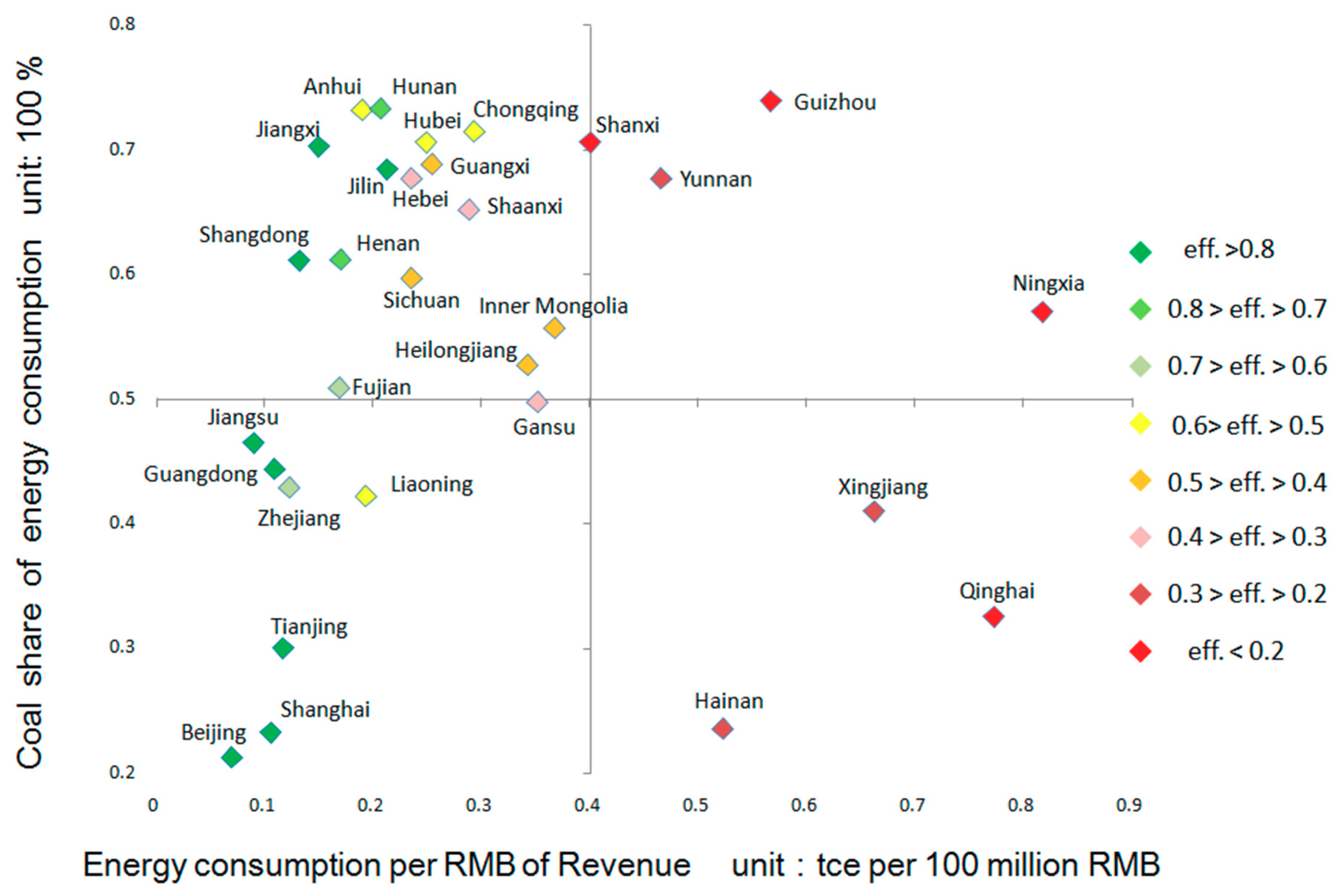
As mentioned above, China’s coal consumption accounted for 62% of the country’s total energy consumption in 2016. Coal as a traditional fossil fuel is the main cause of CO2 emissions. Compared to oil and natural gas, coal contains more impurities such as sulfur and phosphorus, which are the main reasons for the formation of SO2, NOx, and soot (PM2.5). Therefore, coal as a source of energy consumption usually implies an investment of more waste gas treatment costs and a generation of more emissions. The proportion of coal in total energy consumption can be applied to define the energy share of energy consumption in China’s industrial sector. At the same time, when a DMU’s industrial sector relies more on energy consumption to generate revenue, the DMU has higher energy intensity. Thus, the proportion of energy consumption and income are defined as energy consumption per renminbi (RMB) of Revenue.
Figure 6 shows a four-quadrant map of energy efficiency associated with the five-year average of energy consumption structure and energy intensity. We intuitively see that DMUs with a lower coal share and lower energy intensity have higher energy and emission-reduction efficiency values. We further discuss the impact of energy consumption structure and energy intensity on efficiency by comparing data trends over the five-year period.
The next, we compare the changes in energy consumption structure and energy intensity between groups H and L. Table 3 and Table 4 show the results for comparison, and find that the coal share in group H is lower than that in group L in 2011, but only by a difference of 5.3%, showing a downward trend in 2011–2015.The average value of group L did not change significantly over the five years. By 2015, the gap in the coal share between groups H and L had expanded to 14.6%. In group H, the coal share of DMUs in the eastern coastal areas had dropped more significantly.
In terms of energy intensity, group H was significantly lower than group L. The average value of group H declined from 0.151 in 2011 to 0.105 in 2015. The average value of group L has not changed significantly, and has remained around 0.5.
Next, we compare the energy consumption structure and energy intensity changes over the five-year period between groups I and D. Table 5 and Table 6 show the results of the comparison. Table 5 shows that the average coal share values of both groups I and D have decreased over the five years.
The larger difference appears in Table 6. The energy intensity of group I fell from 0.439 in 2011 to 0.283 in 2015. In this group, except for Hainan, the other five DMUs showed a trend of decreasing year by year, of which Guizhou especially experienced a significant decrease. In group D, this indicator had a large increase to 0.409 in 2015 compared to 0.357 in 2011. The indicators of the four DMUs other than Hebei and Heilongjiang in this group showed a significant increasing trend.
Based on the above analysis, reducing the coal share and energy intensity can increase the energy and emission-reduction efficiencies. Those DMUs with higher efficiency values in the eastern coastal areas usually had lower energy intensity and a leading position in promoting the replacement of coal energy consumption structures by clean energy. In comparison, the energy consumption structure adjustment in the central and western regions was relatively slow, and the driving force for increasing the efficiency value in the southwest region was mainly due to the reduction in energy intensity. At the same time, the observations indicate that some DMUs with lower values had a significant increase in energy intensity.
4.2. Emission Treatment Can Reduce Air Pollution, Further Sustainably Promoting the Improvement of Energy and Emission-Reduction Efficiencies
In this model setting, the expenditure on industrial waste gas treatment facilities is taken as an input. On one hand, the increase in the cost will be the cause of the decrease in the efficiency value. On the other hand, the increase in the cost can suppress the increase in the waste gas of the undesirable output, which will bring about an increase in the efficiency value.
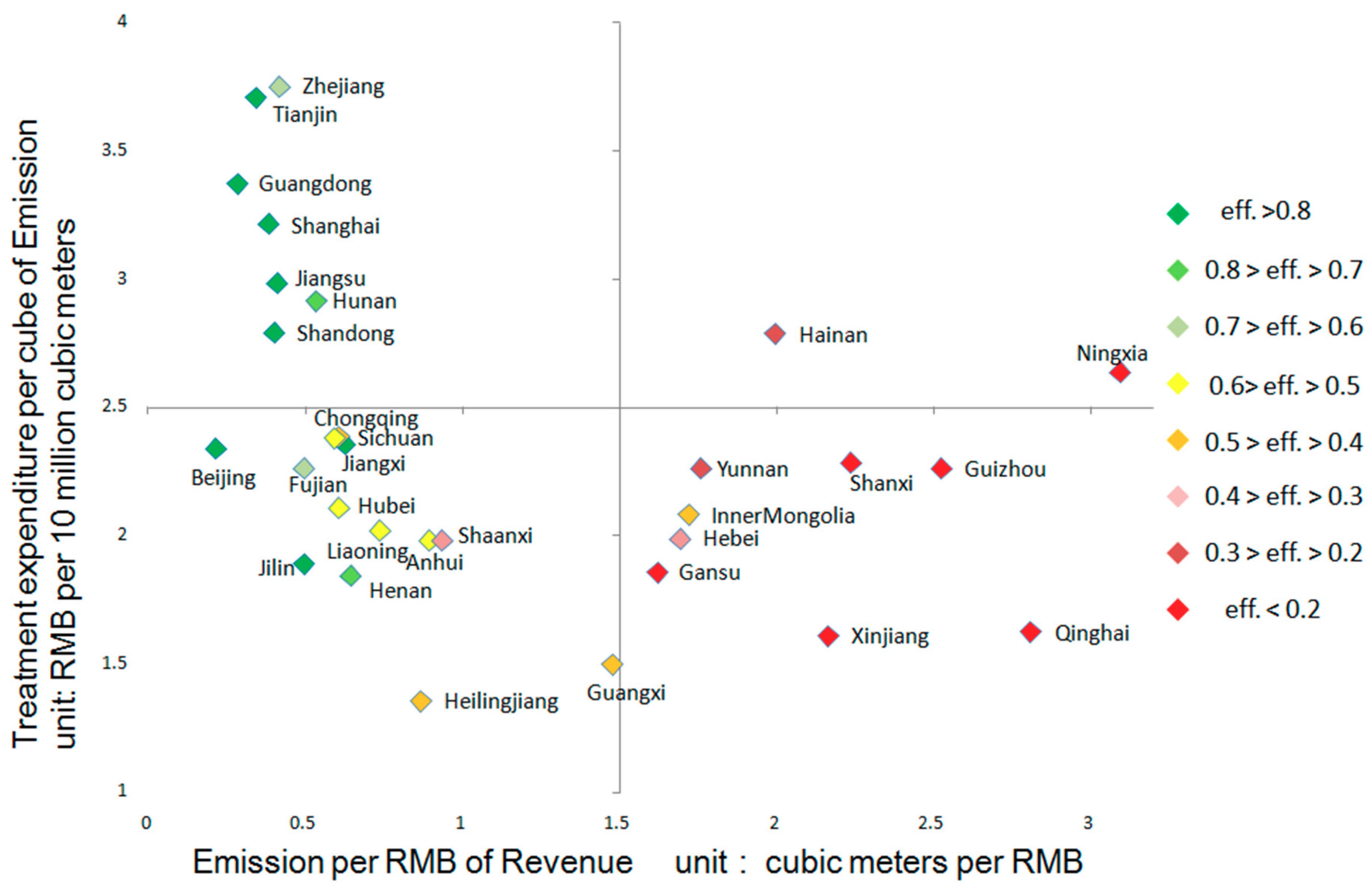
This study aims to find whether or not the emission treatment is conducive to improving the energy and emission-reduction efficiencies. An indicator is set up named ‘treatment intensity’. The definition of expenditure per cubic meter of emissions is from the proportion of waste gas treatment costs and emissions. Moreover, another indicator is set up named ‘emission intensity’, which defined emission per RMB of revenue by the proportion of emissions and revenue. Figure 7 shows the correlation between efficiency values and the five-year average of treatment intensity and emission intensity.
The results show that DMUs that had higher efficiency values usually had lower emission intensity. In fact, most had higher levels of treatment intensity. As a follow-up, we analyzed the trends of these two indicators over the past five years, and discussed the impact on efficiency values.
We compared the changes in treatment intensity and emission intensity between groups H and L over five years. Table 7 and Table 8 list the results of this comparison. The average intensity of treatment for the two groups increased year by year over the five years, while the emission intensity decreased over the five years. However, the treatment intensity of group H was significantly higher than that of group L, while its emission intensity was significantly lower than that of group L. The DMUs with higher efficiency values had high levels of average treatment intensity, and lower levels of average emission intensity. Those DMUs with lower efficiency values have lower average treatment intensity and higher average emission intensity. According to the five years of data, most of the DMUs have increased their investment in waste gas treatment, and their emission intensity has been significantly reduced, such as Jiangxi, Jilin, Ningxia, and Shaanxi.
Next, we compared the change in treatment intensity and emission intensity over the five-year period between the I and D groups. Table 9 and Table 10 present the comparison results, and show that the average treatment intensity of group I increased rapidly over the five years, while the average emission intensity decreased. Some DMUs saw their treatment intensity increase significantly and their emission intensity decrease significantly, such as Chongqing, Guangxi, Hainan, and Hubei. In group I, Guizhou was the only DMU whose treatment intensity did not increase. Combined with the above analysis, the efficiency improvement of Guizhou is mainly due to its reduction in energy intensity. In group D, the average treatment intensity was relatively slow, while the average emission intensity did not show a downward trend. The average emission intensity value in 2015 was higher than that for the previous four years. The emission intensity of some DMUs is more obvious, such as that for Liaoning and Xinjiang.
Based on the above analysis, the DMUs that increased their expenditure on the treatment of industrial waste gas reduced their emission intensity and suppressed the improvement of energy and emission-reduction efficiencies caused by a reduction of undesirable output. This effect is better than the efficiency reduction caused by increased input. The DMUs with higher efficiency values had higher levels of treatment intensity, which was mainly concentrated in the eastern coastal areas. DMUs can reduce their emission intensity by increasing the input of emission treatment, which is an effective way to improve the efficiency value. This is different from Wu et al. [25], who pointed out that Chongqing and Jilin had the lowest energy efficiency. In this study, Jilin, with an efficiency of one as the benchmark, and Chongqing demonstrated a significant increase in efficiency, which was due to the emission intensity decreasing in these two provinces.
5.Conclusions and Policy Recommendations
The Chinese government increased its control over energy conservation and emission reduction in the industrial sector, and achieved improved results over the period 2011–2015. Based on the existing research, we added the expenditure of industrial waste gas treatment as a new input variable, modifying the dynamic SBM model to make it suitable for analysis with undesirable output. Through this, we then estimated the energy and emission-reduction efficiencies of China’s industrial sector over this time.
According to the results, we found that the DMUs with higher efficiency values were mainly distributed in the eastern coastal areas and usually had lower energy intensity. They also took a leading position in the process of energy consumption restructuring by replacing coal with clean energy; these included Beijing, Tianjin, Shanghai, Guangdong, and Jiangsu. In the central and western regions, the adjustment of energy consumption structure was slow, and there was more room for improvement. Some DMUs had improved their efficiency values; this was mainly due to a reduction of energy intensity, and included those of Guizhou, Chongqing, Sichuan, and Hubei. Some DMUs had decreased efficiency values due to the increase in energy intensity, such as Liaoning, Inner Mongolia, Shanxi, and Xinjiang.
For the DMUs that increased their expenditure on the treatment of industrial waste gas in order to reduce air pollution, this effect was better than the energy-efficiency reduction caused by increased input. The DMUs with higher efficiency values typically had higher treatment intensity and lower emission intensity. Some DMUs had higher treatment intensity, and their emission intensity was significantly reduced, thus maintaining high efficiency values or improving their efficiency values; these included Jiangxi, Jilin, Guangxi, and Hainan. Some DMUs had higher or increased emission intensity; those DMUs could increase the expenditure of industrial waste gas treatment as an effective way to reduce air pollution, and thus further sustainably promote the improvement of their energy and emission-reduction efficiencies. This includes the DMUs of Guizhou, Qinghai, Xinjiang, Inner Mongolia, and Shanxi.
Author Contributions
Conceptualization, X.T. and Y.-h.C.; methodology, Y.-h.C.; software, X.T.; validation, X.T., Y.-h.C. and L.C.L.; formal analysis, X.T.; investigation, X.T.; resources, X.T.; data curation, X.T.; writing—original draft preparation, X.T.; writing—review and editing, L.C.L.; visualization, X.T.; supervision, Y.-h.C.; project administration, Y.-h.C.; funding acquisition, X.T.
Funding
This research received no external funding.
Conflicts of Interest
The authors declare no conflict of interest.
References
- Enerdata. Global Energy Statistical Yearbook 2017. 2017. Available online: https://yearbook.enerdata.net/total-energy/world-consumption-statistics.html (accessed on 6 November 2018).
- National Bureau of Statistics of China. China Statistical Yearbook 2017. 2017. Available online: http://www.stats.gov.cn/tjsj/ndsj/2017/indexeh.htm (accessed on 6 November 2018).
- The Health Effects Institute (HEI). State of Global Air, 2017: A Special Report on Global Exposure to Air Pollution and Its Disease Burden. 2017. Available online: https://www.stateofglobalair.org/sites/default/files/SOGA2017_report.pdf (accessed on 6 November 2018).
- The HINDU. India’s Pollution Levels Beat China’s: Study. 2016. Available online: http://www.thehindu.com/news/cities/Delhi/indias-pollution-levels-beat-chinas-study/article8269631.ece (accessed on 6 November 2018).
- Färe, R.; Grosskopf, S.; Tyteca, D. An activity analysis model of the environmental performance of firms—Application to fossil-fuel-fired electric utilities. Ecol. Econ. 1996, 18, 161–175. [Google Scholar] [CrossRef]
- Zaim, O.; Taskin, F. A Kuznets curve in environmental efficiency: An application on OECD countries. Environ. Resour. Econ. 2000, 17, 21–36. [Google Scholar] [CrossRef]
- Färe, R.; Grosskopf, S.; Hernandez-Sancho, F. Environmental performance: An index number approach. Resour. Energy Econ. 2004, 26, 343–352. [Google Scholar] [CrossRef]
- Zhou, P.; Ang, B.W. Decomposition of aggregate CO2 emissions: A production-theoretical approach. Energy Econ. 2008, 30, 1054–1067. [Google Scholar] [CrossRef]
- Hu, J.L.; Wang, S.C. Total-factor energy efficiency of regions in China. Energy Policy 2006, 34, 3206–3217. [Google Scholar] [CrossRef]
- Wei, C.; Ni, J.; Shen, M. Empirical analysis of provincial energy efficiency in China. China World Econ. 2009, 17, 88–103. [Google Scholar] [CrossRef]
- Chang, T.P.; Hu, J.L. Total-factor energy productivity growth, technical progress, and efficiency change: An empirical study of China. Appl. Energy 2010, 87, 3262–3270. [Google Scholar] [CrossRef]
- Zou, G.; Chen, L.; Liu, W.; Hong, X.; Zhang, G.; Zhang, Z. Measurement and evaluation of Chinese regional energy efficiency based on provincial panel data. Math. Comput. Model. 2013, 58, 1000–1009. [Google Scholar] [CrossRef]
- Li, K.; Lin, B. Metafroniter energy efficiency with CO2 emissions and its convergence analysis for China. Energy Econ. 2015, 48, 230–241. [Google Scholar] [CrossRef]
- Zhou, D.Q.; Meng, F.Y.; Bai, Y.; Cai, S.Q. Energy efficiency and congestion assessment with energy mix effect: The case of APEC countries. J. Clean. Prod. 2017, 142, 819–828. [Google Scholar] [CrossRef]
- Choi, Y.; Zhang, N.; Zhou, P. Efficiency and abatement costs of energy-related CO2 emissions in China: A slacks-based efficiency measure. Appl. Energy 2012, 98, 198–208. [Google Scholar] [CrossRef]
- Wang, K.; Wei, Y.M.; Zhang, X. A comparative analysis of China’s regional energy and emission performance: Which is the better way to deal with undesirable outputs? Energy Policy 2012, 46, 574–584. [Google Scholar] [CrossRef]
- Wang, K.; Lu, B.; Wei, Y.M. China’s regional energy and environmental efficiency: A range-adjusted measure based analysis. Appl. Energy 2013, 112, 1403–1415. [Google Scholar] [CrossRef]
- Yeh, T.L.; Chen, T.Y.; Lai, P.Y. A comparative study of energy utilization efficiency between Taiwan and China. Energy Policy 2010, 38, 2386–2394. [Google Scholar] [CrossRef]
- Wang, Z.; Feng, C. A performance evaluation of the energy, environmental, and economic efficiency and productivity in China: An application of global data envelopment analysis. Appl. Energy 2015, 147, 617–626. [Google Scholar] [CrossRef]
- Zhang, N.; Choi, Y. Environmental energy efficiency of China’s regional economies: A non-oriented slacks-based measure analysis. Soc. Sci. J. 2013, 50, 225–234. [Google Scholar] [CrossRef]
- Yu, Y.; Choi, Y. Measuring environmental performance under regional heterogeneity in China: Ametafrontier efficiency analysis. Comput. Econ. 2015, 46, 375–388. [Google Scholar] [CrossRef]
- Kao, C. Dynamic data envelopment analysis: A relational analysis. Eur. J. Oper. Res. 2013, 227, 325–330. [Google Scholar] [CrossRef]
- Sueyoshi, T.; Goto, M.; Sugiyama, M. DEA window analysis for environmental assessment in a dynamic time shift: Performance assessment of US coal-fired power plants. Energy Econ. 2013, 40, 845–857. [Google Scholar] [CrossRef]
- Wang, K.; Yu, S.; Zhang, W. China’s regional energy and environmental efficiency: A DEA window analysis based dynamic evaluation. Math. Comput. Model. 2013, 58, 1117–1127. [Google Scholar] [CrossRef]
- Wu, A.H.; Cao, Y.Y.; Liu, B. Energy efficiency evaluation for regions in China: An application of DEA and Malmquist indices. Energy Effic. 2014, 7, 429–439. [Google Scholar] [CrossRef]
- Yao, X.; Guo, C.; Shao, S.; Jiang, Z. Total-factor CO2 emission performance of China’s provincial industrial sector: A meta-frontier non-radial Malmquist index approach. Appl. Energy 2016, 184, 1142–1153. [Google Scholar] [CrossRef]
- Wu, J.; Zhu, Q.; Yin, P.; Song, M. Measuring energy and environmental performance for regions in China by using DEA-based Malmquist indices. Oper. Res. 2017, 17, 715–735. [Google Scholar] [CrossRef]
- Tone, K.; Tsutsui, M. Dynamic DEA: A slacks-based measure approach. Omega 2010, 38, 145–156. [Google Scholar] [CrossRef]
- Guo, X.; Lu, C.; Lee, J. Applying the dynamic DEA model to evaluate the energy efficiency of OECD countries and China. Energy 2017, 134, 392–399. [Google Scholar] [CrossRef]
- Ke, T. Energy efficiency of APEC members—Applied dynamic SBM model. Carbon Manag. 2017, 8, 293–303. [Google Scholar] [CrossRef]
- Cole, M.; Elliott, R.J.; Wu, S. Industrial activity and the environment in China: An industry-level analysis. China Econ. Rev. 2008, 19, 393–408. [Google Scholar] [CrossRef]
- Wang, S.S.; Zhou, D.Q.; Zhou, P.; Wang, Q.W. CO2 emissions, energy consumption and economic growth in China: A panel data analysis. Energy Policy 2011, 39, 4870–4875. [Google Scholar] [CrossRef]
- Yang, M.; Patino-Echeverri, D.; Yang, F.; Williams, E. Industrial energy efficiency in China: Achievements, challenges and opportunities. Energy Strategy Rev. 2015, 6, 20–29. [Google Scholar] [CrossRef]
- Dong, K.Y.; Sun, R.J.; Li, H.; Jiang, H.D. A review of China’s energy consumption structure and outlook based on a long-range energy alternatives modeling tool. Pet. Sci. 2017, 14, 214–227. [Google Scholar] [CrossRef]
- Färe, R.; Grosskopf, S.; Norris, M. Productivity growth, technical progress, and efficiency change in industrialized countries: Reply. Am. Econ. Rev. 1997, 87, 1040–1044. [Google Scholar]
- Färe, R.; Grosskopf, S. Productivity and intermediate products: A frontier approach. Econ. Lett. 1996, 50, 65–70. [Google Scholar] [CrossRef] [Green Version]
- Department of Industry Statistical, National Bureau of Statistics of China. China Industry Statistical Yearbook, 2012; China Statistics Press: Beijing, China, 2012; Volume 1.
- Department of Industry Statistical, National Bureau of Statistics of China. China Industry Statistical Yearbook, 2013; China Statistics Press: Beijing, China, 2013; Volume 1.
- Department of Industry Statistical, National Bureau of Statistics of China. China Industry Statistical Yearbook, 2014; China Statistics Press: Beijing, China, 2014; Volume 1.
- Department of Industry Statistical, National Bureau of Statistics of China. China Industry Statistical Yearbook, 2015; China Statistics Press: Beijing, China, 2015; Volume 1.
- Department of Industry Statistical, National Bureau of Statistics of China. China Industry Statistical Yearbook, 2016; China Statistics Press: Beijing, China, 2016; Volume 1.
- Department of Energy Statistical, National Bureau of Statistics of China. China Energy Statistical Yearbook, 2012; China Statistics Press: Beijing, China, 2012.
- Department of Energy Statistical, National Bureau of Statistics of China. China Energy Statistical Yearbook, 2013; China Statistics Press: Beijing, China, 2013.
- Department of Energy Statistical, National Bureau of Statistics of China. China Energy Statistical Yearbook, 2014; China Statistics Press: Beijing, China, 2014.
- Department of Energy Statistical, National Bureau of Statistics of China. China Energy Statistical Yearbook, 2015; China Statistics Press: Beijing, China, 2015.
- Department of Energy Statistical, National Bureau of Statistics of China. China Energy Statistical Yearbook, 2016; China Statistics Press: Beijing, China, 2016.
- National Bureau of Statistics of China; National Bureau of Statistics Ministry of Environmental Protection. China Statistical Yearbook on Environment, 2012; China Statistics Press: Beijing, China, 2012.
- National Bureau of Statistics of China; National Bureau of Statistics Ministry of Environmental Protection. China Statistical Yearbook on Environment, 2013; China Statistics Press: Beijing, China, 2013.
- National Bureau of Statistics of China; National Bureau of Statistics Ministry of Environmental Protection. China Statistical Yearbook on Environment, 2014; China Statistics Press: Beijing, China, 2014.
- National Bureau of Statistics of China; National Bureau of Statistics Ministry of Environmental Protection. China Statistical Yearbook on Environment, 2015; China Statistics Press: Beijing, China, 2015.
- National Bureau of Statistics of China; National Bureau of Statistics Ministry of Environmental Protection. China Statistical Yearbook on Environment, 2016; China Statistics Press: Beijing, China, 2016.
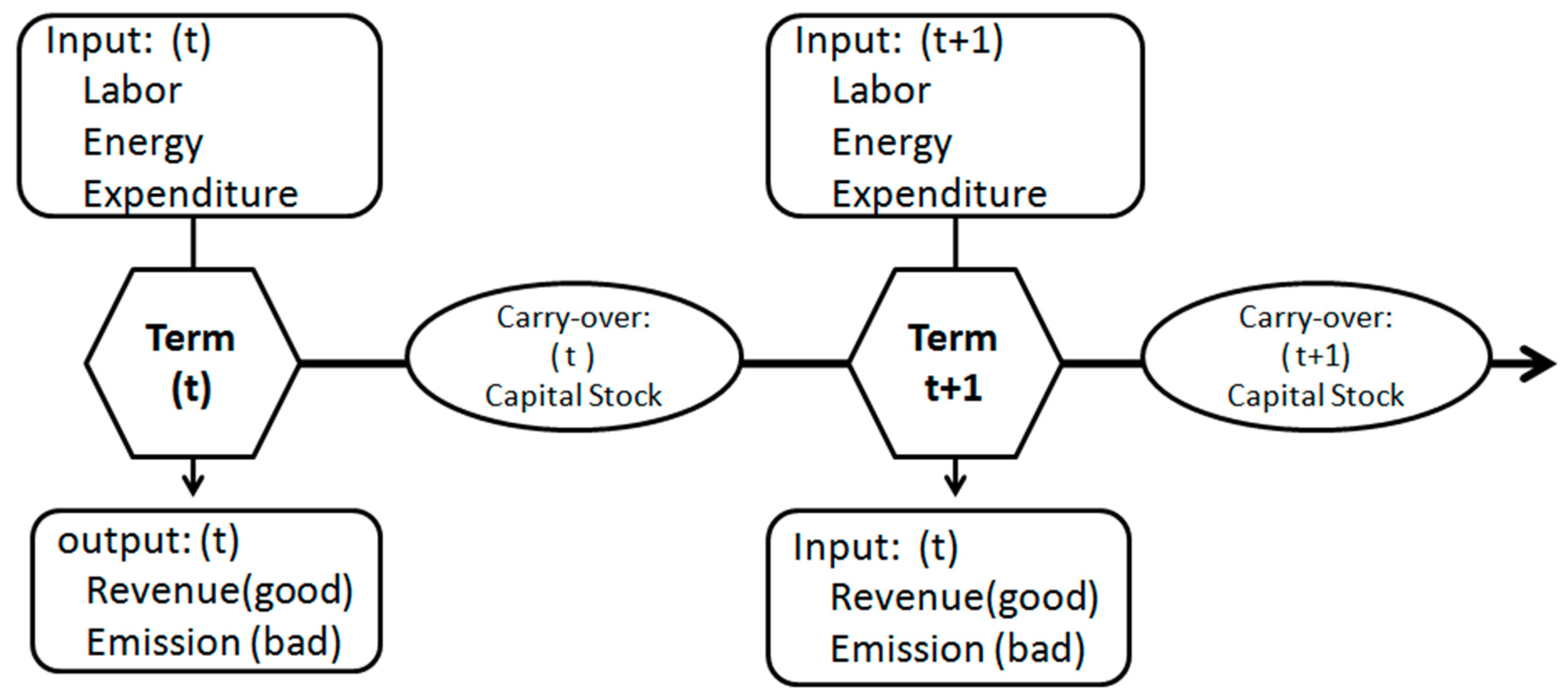
Figure 1.
Thegeneral overview of variables, carry-over, and dynamic slacks-based measure (SBM) model.
Figure 1.
Thegeneral overview of variables, carry-over, and dynamic slacks-based measure (SBM) model.

Figure 2.
The trends of facilities and expenditure from 2011–2015.

Figure 3.
The trends of capital stock and revenue from 2011–2015.

Figure 4.
Energy and emission-reduction efficiencies in 2011.

Figure 5.
Energy and emission-reduction efficiencies in 2015.

Figure 6.
Efficiency values depending on energy consumption structure and energy intensity.

Figure 7.
Efficiency values depending on treatment intensity and emission intensity.


Table 1.
Descriptive statistics of variables and carry-over.
| Year | Variable and Carry-Over | Unit | Average | SD | Min | Max |
|---|---|---|---|---|---|---|
| 2011 | (I)Labor | million persons | 3.148 | 3.273 | 0.181 | 14.511 |
| (I)Energy | million tce | 58.841 | 36.713 | 8.636 | 163.490 | |
| (I)Expenditure | billion RMB | 4.459 | 3.552 | 0.371 | 14.390 | |
| (O)Revenue | trillion RMB | 2.806 | 2.799 | 0.160 | 10.703 | |
| (OB)Emission | trillion cubic meters | 2.248 | 1.657 | 0.168 | 7.718 | |
| (C)Capital stock | trillion RMB | 2.252 | 1.872 | 0.175 | 7.626 | |
| 2012 | (I)Labor | million persons | 3.224 | 3.588 | 0.122 | 15.576 |
| (I)Energy | million tce | 60.892 | 36.621 | 8.522 | 170.668 | |
| (I)Expenditure | billion RMB | 4.840 | 4.565 | 0.556 | 22.438 | |
| (O)Revenue | trillion RMB | 3.097 | 3.085 | 0.170 | 11.929 | |
| (OB)Emission | trillion cubic meters | 2.118 | 1.474 | 0.196 | 6.765 | |
| (C)Capital stock | trillion RMB | 2.560 | 2.056 | 0.202 | 8.455 | |
| 2013 | (I)Labor | million persons | 3.262 | 3.426 | 0.127 | 14.558 |
| (I)Energy | million tce | 57.990 | 34.370 | 8.606 | 161.11 | |
| (I)Expenditure | billion RMB | 4.992 | 3.640 | 0.364 | 13.316 | |
| (O)Revenue | trillion RMB | 3.430 | 3.423 | 0.164 | 13.232 | |
| (OB)Emission | trillion cubic meters | 2.231 | 1.615 | 0.369 | 7.912 | |
| (C)Capital | trillion RMB | 2.834 | 2.240 | 0.233 | 9.208 | |
| 2014 | (I)Labor | million persons | 3.325 | 3.458 | 0.116 | 14.705 |
| (I)Energy | million tce | 59.292 | 35.435 | 8.973 | 174.868 | |
| (I)Expenditure | billion RMB | 5.769 | 4.349 | 0.687 | 16.352 | |
| (O)Revenue | trillion RMB | 3.690 | 3.706 | 0.176 | 14.314 | |
| (OB)Emission | trillion cube | 2.313 | 1.648 | 0.264 | 7.273 | |
| (C)Capital | trillion RMB | 3.187 | 2.514 | 0.244 | 10.126 | |
| 2015 | (I)Labor | million persons | 3.257 | 3.451 | 0.116 | 14.638 |
| (I)Energy | million tce | 59.374 | 33.434 | 8.762 | 156.134 | |
| (I)Expenditure | billion RMB | 6.219 | 4.713 | 0.732 | 18.435 | |
| (O)Revenue | trillion RMB | 3.699 | 3.826 | 0.166 | 14.707 | |
| (OB)Emission | trillion cubic meters | 2.229 | 1.721 | 0.234 | 7.857 | |
| (C)Capital | trillion RMB | 3.408 | 2.686 | 0.279 | 10.706 |
Table 2.
Energy and emission-reduction efficiency values by dynamic SBM model from 2011–2015. DMU: decision-making unit.
Table 2.
Energy and emission-reduction efficiency values by dynamic SBM model from 2011–2015. DMU: decision-making unit.
| DMU | Score | 2011 | 2012 | 2013 | 2014 | 2015 | Rank | Group |
|---|---|---|---|---|---|---|---|---|
| Anhui | 0.503 | 0.497 | 0.507 | 0.477 | 0.514 | 0.519 | 16 | □ |
| Beijing | 1 | 1 | 1 | 1 | 1 | 1 | 1 | H |
| Chongqing | 0.512 | 0.466 | 0.431 | 0.429 | 0.575 | 0.685 | 15 | I |
| Fujian | 0.658 | 0.729 | 0.638 | 0.555 | 0.659 | 0.719 | 11 | □ |
| Gansu | 0.331 | 0.336 | 0.344 | 0.328 | 0.332 | 0.313 | 23 | L |
| Guangdong | 1 | 1 | 1 | 1 | 1 | 1 | 1 | H |
| Guangxi | 0.426 | 0.372 | 0.401 | 0.398 | 0.472 | 0.497 | 19 | I |
| Guizhou | 0.194 | 0.162 | 0.168 | 0.168 | 0.211 | 0.262 | 29 | I |
| Hainan | 0.265 | 0.152 | 0.245 | 0.286 | 0.291 | 0.346 | 24 | I |
| Hebei | 0.392 | 0.441 | 0.422 | 0.381 | 0.367 | 0.352 | 21 | L/D |
| Heilongjiang | 0.424 | 0.497 | 0.469 | 0.426 | 0.411 | 0.322 | 20 | D |
| Henan | 0.753 | 1 | 0.658 | 0.647 | 0.700 | 0.810 | 9 | □ |
| Hubei | 0.575 | 0.528 | 0.561 | 0.567 | 0.601 | 0.624 | 14 | I |
| Hunan | 0.711 | 0.796 | 0.662 | 0.789 | 0.707 | 0.602 | 10 | □ |
| Inner Mongolia | 0.429 | 1 | 0.382 | 0.327 | 0.314 | 0.294 | 18 | D |
| Jiangsu | 1 | 1 | 1 | 1 | 1 | 1 | 1 | H |
| Jiangxi | 1 | 1 | 1 | 1 | 1 | 1 | 1 | H |
| Jilin | 1 | 1 | 1 | 1 | 1 | 1 | 1 | H |
| Liaoning | 0.599 | 0.746 | 0.673 | 0.696 | 0.583 | 0.340 | 13 | D |
| Ningxia | 0.184 | 0.181 | 0.202 | 0.181 | 0.179 | 0.175 | 30 | L |
| Qinghai | 0.194 | 0.225 | 0.206 | 0.174 | 0.190 | 0.177 | 28 | L |
| Shaanxi | 0.357 | 0.378 | 0.385 | 0.333 | 0.349 | 0.341 | 22 | L |
| Shandong | 1 | 1 | 1 | 1 | 1 | 1 | 1 | H |
| Shanghai | 0.949 | 1 | 1 | 1 | 1 | 0.761 | 8 | H |
| Shanxi | 0.198 | 0.239 | 0.240 | 0.190 | 0.170 | 0.152 | 27 | L/D |
| Sichuan | 0.492 | 0.446 | 0.456 | 0.447 | 0.539 | 0.585 | 17 | I |
| Tianjin | 1 | 1 | 1 | 1 | 1 | 1 | 1 | H |
| Xinjiang | 0.256 | 0.323 | 0.273 | 0.247 | 0.231 | 0.210 | 25 | L/D |
| Yunnan | 0.226 | 0.231 | 0.243 | 0.212 | 0.223 | 0.222 | 26 | L |
| Zhejiang | 0.608 | 0.625 | 0.637 | 0.565 | 0.585 | 0.635 | 12 | □ |
| Average | 0.575 | 0.612 | 0.577 | 0.561 | 0.573 | 0.561 | □ | □ |
| Max | 1 | 1 | 1 | 1 | 1 | 1 | □ | □ |
| Min | 0.184 | 0.152 | 0.168 | 0.168 | 0.170 | 0.152 | □ | □ |
| St. Dev. | 0.299 | 0.321 | 0.295 | 0.310 | 0.304 | 0.307 | □ | □ |
Table 3.
Comparing the coal share of energy consumption between the H (High-efficiency) and L (Low-efficiency)groups, unit: 100%.
Table 3.
Comparing the coal share of energy consumption between the H (High-efficiency) and L (Low-efficiency)groups, unit: 100%.
| Group H | 2011 | 2012 | 2013 | 2014 | 2015 | Group L | 2011 | 2012 | 2013 | 2014 | 2015 |
|---|---|---|---|---|---|---|---|---|---|---|---|
| Beijing | 0.296 | 0.273 | 0.238 | 0.197 | 0.148 | Gansu | 0.484 | 0.504 | 0.474 | 0.492 | 0.505 |
| Guangdong | 0.472 | 0.467 | 0.408 | 0.430 | 0.425 | Hebei | 0.671 | 0.687 | 0.677 | 0.688 | 0.669 |
| Jiangsu | 0.534 | 0.487 | 0.454 | 0.430 | 0.435 | Ningxia | 0.527 | 0.524 | 0.535 | 0.582 | 0.607 |
| Jiangxi | 0.702 | 0.708 | 0.682 | 0.694 | 0.703 | Qinghai | 0.235 | 0.289 | 0.286 | 0.292 | 0.345 |
| Jilin | 0.741 | 0.725 | 0.665 | 0.667 | 0.643 | Shaanxi | 0.645 | 0.679 | 0.635 | 0.635 | 0.665 |
| Shandong | 0.665 | 0.675 | 0.614 | 0.636 | 0.538 | Shanxi | 0.693 | 0.686 | 0.718 | 0.721 | 0.709 |
| Shanghai | 0.271 | 0.233 | 0.222 | 0.244 | 0.207 | Xinjiang | 0.518 | 0.519 | 0.380 | 0.316 | 0.347 |
| Tianjin | 0.342 | 0.333 | 0.309 | 0.306 | 0.260 | Yunnan | 0.679 | 0.674 | 0.697 | 0.673 | 0.680 |
| Average | 0.503 | 0.488 | 0.449 | 0.450 | 0.420 | Average | 0.556 | 0.570 | 0.550 | 0.550 | 0.566 |
Table 4.
Comparing the energy intensity between the H and L groups, unit: tce per 100 million renminbi (RMB).
Table 4.
Comparing the energy intensity between the H and L groups, unit: tce per 100 million renminbi (RMB).
| Group H | 2011 | 2012 | 2013 | 2014 | 2015 | Group L | 2011 | 2012 | 2013 | 2014 | 2015 |
|---|---|---|---|---|---|---|---|---|---|---|---|
| Beijing | 0.095 | 0.086 | 0.057 | 0.057 | 0.057 | Gansu | 0.380 | 0.369 | 0.348 | 0.323 | 0.338 |
| Guangdong | 0.124 | 0.122 | 0.108 | 0.096 | 0.094 | Hebei | 0.259 | 0.248 | 0.223 | 0.223 | 0.223 |
| Jiangsu | 0.106 | 0.095 | 0.088 | 0.079 | 0.079 | Ningxia | 0.873 | 0.737 | 0.877 | 0.746 | 0.852 |
| Jiangxi | 0.176 | 0.158 | 0.159 | 0.128 | 0.129 | Qinghai | 0.757 | 0.830 | 0.888 | 0.753 | 0.837 |
| Jilin | 0.304 | 0.261 | 0.164 | 0.179 | 0.161 | Shaanxi | 0.309 | 0.303 | 0.282 | 0.271 | 0.278 |
| Shandong | 0.164 | 0.145 | 0.118 | 0.122 | 0.107 | Shanxi | 0.364 | 0.352 | 0.381 | 0.416 | 0.486 |
| Shanghai | 0.108 | 0.105 | 0.105 | 0.104 | 0.106 | Xinjiang | 0.584 | 0.669 | 0.703 | 0.620 | 0.737 |
| Tianjin | 0.130 | 0.123 | 0.115 | 0.110 | 0.111 | Yunnan | 0.525 | 0.473 | 0.449 | 0.438 | 0.447 |
| Average | 0.151 | 0.137 | 0.114 | 0.109 | 0.105 | Average | 0.506 | 0.498 | 0.519 | 0.474 | 0.525 |
Table 5.
Comparing the coal share of energy consumption between the I (Increased efficiency) and D(Decreased efficiency) groups, unit:100%.
Table 5.
Comparing the coal share of energy consumption between the I (Increased efficiency) and D(Decreased efficiency) groups, unit:100%.
| Group I | 2011 | 2012 | 2013 | 2014 | 2015 | Group D | 2011 | 2012 | 2013 | 2014 | 2015 |
|---|---|---|---|---|---|---|---|---|---|---|---|
| Chongqing | 0.725 | 0.751 | 0.660 | 0.695 | 0.701 | Hebei | 0.671 | 0.687 | 0.677 | 0.688 | 0.669 |
| Guangxi | 0.725 | 0.728 | 0.692 | 0.678 | 0.655 | Heilongjiang | 0.532 | 0.544 | 0.539 | 0.553 | 0.503 |
| Guizhou | 0.746 | 0.775 | 0.661 | 0.766 | 0.704 | Inner Mongolia | 0.594 | 0.515 | 0.545 | 0.523 | 0.576 |
| Hainan | 0.241 | 0.281 | 0.245 | 0.228 | 0.215 | Liaoning | 0.439 | 0.407 | 0.467 | 0.459 | 0.403 |
| Hubei | 0.790 | 0.807 | 0.677 | 0.640 | 0.647 | Shanxi | 0.693 | 0.686 | 0.718 | 0.721 | 0.709 |
| Sichuan | 0.614 | 0.686 | 0.586 | 0.642 | 0.522 | Xinjiang | 0.518 | 0.519 | 0.347 | 0.316 | 0.347 |
| Average | 0.640 | 0.671 | 0.587 | 0.608 | 0.574 | Average | 0.574 | 0.560 | 0.549 | 0.543 | 0.535 |
Table 6.
Comparing the energy intensity between the I and D groups, unit: tce per 100 million RMB.
| Group I | 2011 | 2012 | 2013 | 2014 | 2015 | Group D | 2011 | 2012 | 2013 | 2014 | 2015 |
|---|---|---|---|---|---|---|---|---|---|---|---|
| Chongqing | 0.398 | 0.334 | 0.291 | 0.230 | 0.214 | Hebei | 0.259 | 0.248 | 0.223 | 0.223 | 0.223 |
| Guangxi | 0.330 | 0.291 | 0.236 | 0.219 | 0.193 | Heilongjiang | 0.367 | 0.355 | 0.305 | 0.333 | 0.354 |
| Guizhou | 0.758 | 0.765 | 0.535 | 0.409 | 0.372 | Inner Mongolia | 0.368 | 0.315 | 0.396 | 0.350 | 0.409 |
| Hainan | 0.539 | 0.502 | 0.534 | 0.511 | 0.527 | Liaoning | 0.200 | 0.198 | 0.154 | 0.170 | 0.242 |
| Hubei | 0.353 | 0.328 | 0.199 | 0.187 | 0.174 | Shanxi | 0.364 | 0.352 | 0.381 | 0.416 | 0.486 |
| Sichuan | 0.257 | 0.279 | 0.235 | 0.190 | 0.214 | Xinjiang | 0.584 | 0.669 | 0.703 | 0.620 | 0.737 |
| Average | 0.439 | 0.416 | 0.338 | 0.291 | 0.283 | Average | 0.357 | 0.356 | 0.360 | 0.352 | 0.409 |
Table 7.
Comparing treatment intensity between the H and L groups, unit: RMB per 10 million cubic meters.
Table 7.
Comparing treatment intensity between the H and L groups, unit: RMB per 10 million cubic meters.
| Group H | 2011 | 2012 | 2013 | 2014 | 2015 | Group L | 2011 | 2012 | 2013 | 2014 | 2015 |
|---|---|---|---|---|---|---|---|---|---|---|---|
| Beijing | 1.689 | 2.692 | 2.439 | 2.880 | 1.990 | Gansu | 1.561 | 1.485 | 1.819 | 2.273 | 2.142 |
| Guangdong | 2.826 | 3.348 | 3.731 | 3.629 | 3.324 | Hebei | 1.864 | 1.929 | 1.683 | 2.248 | 2.216 |
| Jiangsu | 2.366 | 4.615 | 2.549 | 2.577 | 2.813 | Ningxia | 2.085 | 2.220 | 2.735 | 2.593 | 3.537 |
| Jiangxi | 1.948 | 2.245 | 2.423 | 2.494 | 2.666 | Qinghai | 1.225 | 1.556 | 1.727 | 1.686 | 1.910 |
| Jilin | 1.310 | 1.433 | 1.978 | 2.453 | 2.272 | Shaanxi | 1.426 | 1.872 | 1.960 | 2.197 | 2.461 |
| Shandong | 2.317 | 2.516 | 2.775 | 3.099 | 3.245 | Shanxi | 2.095 | 1.820 | 2.087 | 2.781 | 2.637 |
| Shanghai | 3.037 | 3.031 | 3.533 | 3.104 | 3.378 | Xinjiang | 1.213 | 1.344 | 1.545 | 2.200 | 1.733 |
| Tianjin | 4.890 | 2.853 | 3.175 | 3.594 | 4.010 | Yunnan | 1.720 | 2.459 | 2.486 | 2.477 | 2.166 |
| Average | 2.548 | 2.842 | 2.825 | 2.979 | 2.962 | Average | 1.649 | 1.836 | 2.005 | 2.307 | 2.350 |
Table 8.
Comparing emission intensity between the H and L groups, unit: cubic meters per RMB.
| Group H | 2011 | 2012 | 2013 | 2014 | 2015 | Group L | 2011 | 2012 | 2013 | 2014 | 2015 |
|---|---|---|---|---|---|---|---|---|---|---|---|
| Beijing | 0.311 | 0.193 | 0.198 | 0.180 | 0.195 | Gansu | 1.963 | 1.785 | 1.501 | 1.325 | 1.530 |
| Guangdong | 0.338 | 0.289 | 0.274 | 0.258 | 0.256 | Hebei | 1.920 | 1.550 | 1.729 | 1.541 | 1.721 |
| Jiangsu | 0.450 | 0.408 | 0.376 | 0.420 | 0.394 | Ningxia | 4.146 | 3.127 | 2.640 | 3.039 | 2.522 |
| Jiangxi | 0.867 | 0.657 | 0.583 | 0.502 | 0.518 | Qinghai | 3.034 | 2.915 | 2.748 | 2.866 | 2.490 |
| Jilin | 0.635 | 0.520 | 0.447 | 0.405 | 0.471 | Shaanxi | 1.139 | 0.904 | 0.916 | 0.847 | 0.879 |
| Shandong | 0.506 | 0.385 | 0.356 | 0.364 | 0.390 | Shanxi | 2.511 | 2.104 | 2.243 | 2.024 | 2.306 |
| Shanghai | 0.400 | 0.392 | 0.386 | 0.367 | 0.375 | Xinjiang | 1.750 | 2.113 | 2.145 | 2.373 | 2.449 |
| Tianjin | 0.423 | 0.382 | 0.299 | 0.310 | 0.299 | Yunnan | 2.302 | 1.672 | 1.633 | 1.609 | 1.582 |
| Average | 0.491 | 0.403 | 0.365 | 0.351 | 0.362 | Average | 2.345 | 2.021 | 1.944 | 1.953 | 1.935 |
Table 9.
Comparing treatment intensity between groups I and D, unit: RMB per 10 million cubic meters.
Table 9.
Comparing treatment intensity between groups I and D, unit: RMB per 10 million cubic meters.
| Group I | 2011 | 2012 | 2013 | 2014 | 2015 | Group D | 2011 | 2012 | 2013 | 2014 | 2015 |
|---|---|---|---|---|---|---|---|---|---|---|---|
| Chongqing | 1.820 | 2.426 | 2.431 | 2.723 | 2.507 | Hebei | 1.864 | 1.929 | 1.683 | 2.248 | 2.216 |
| Guangxi | 0.853 | 0.986 | 1.420 | 1.808 | 2.417 | Heilongjiang | 1.240 | 1.232 | 1.402 | 1.280 | 1.616 |
| Guizhou | 3.028 | 2.524 | 1.707 | 1.900 | 2.148 | Inner Mongolia | 1.730 | 2.123 | 2.107 | 2.093 | 2.348 |
| Hainan | 2.216 | 2.835 | 2.771 | 2.604 | 3.494 | Liaoning | 1.831 | 1.903 | 1.935 | 2.054 | 2.385 |
| Hubei | 1.541 | 1.817 | 2.292 | 2.447 | 2.447 | Shanxi | 2.095 | 1.820 | 2.087 | 2.781 | 2.637 |
| Sichuan | 2.446 | 1.958 | 2.398 | 2.352 | 2.743 | Xinjiang | 1.213 | 1.344 | 1.545 | 2.200 | 1.733 |
| Average | 1.984 | 2.091 | 2.170 | 2.306 | 2.626 | Average | 1.662 | 1.725 | 1.793 | 2.109 | 2.156 |
Table 10.
Comparing emission intensity between groups I and D, unit: cubic meters per RMB.
| Group I | 2011 | 2012 | 2013 | 2014 | 2015 | Group D | 2011 | 2012 | 2013 | 2014 | 2015 |
|---|---|---|---|---|---|---|---|---|---|---|---|
| Chongqing | 0.801 | 0.649 | 0.618 | 0.497 | 0.475 | Hebei | 1.920 | 1.550 | 1.729 | 1.541 | 1.721 |
| Guangxi | 2.444 | 1.874 | 1.278 | 0.985 | 0.820 | Heilongjiang | 0.906 | 0.834 | 0.783 | 0.902 | 0.925 |
| Guizhou | 2.155 | 2.399 | 3.557 | 2.681 | 1.852 | Inner Mongolia | 1.714 | 1.551 | 1.592 | 1.847 | 1.895 |
| Hainan | 2.046 | 2.155 | 2.877 | 1.502 | 1.408 | Liaoning | 0.740 | 0.662 | 0.565 | 0.708 | 1.023 |
| Hubei | 0.843 | 0.604 | 0.528 | 0.524 | 0.548 | Shanxi | 2.511 | 2.104 | 2.243 | 2.024 | 2.306 |
| Sichuan | 0.775 | 0.697 | 0.561 | 0.527 | 0.428 | Xinjiang | 1.750 | 2.113 | 2.145 | 2.373 | 2.449 |
| Average | 1.511 | 1.396 | 1.570 | 1.119 | 0.922 | Average | 1.590 | 1.469 | 1.509 | 1.566 | 1.720 |
© 2018 by the authors. Licensee MDPI, Basel, Switzerland. This article is an open access article distributed under the terms and conditions of the Creative Commons Attribution (CC BY) license (http://creativecommons.org/licenses/by/4.0/).
Share and Cite
MDPI and ACS Style
Teng, X.; Lu, L.C.; Chiu, Y.-h. Considering Emission Treatment for Energy-Efficiency Improvement and Air Pollution Reduction in China’s Industrial Sector. Sustainability 2018, 10, 4329. https://doi.org/10.3390/su10114329
AMA Style
Teng X, Lu LC, Chiu Y-h. Considering Emission Treatment for Energy-Efficiency Improvement and Air Pollution Reduction in China’s Industrial Sector. Sustainability. 2018; 10(11):4329. https://doi.org/10.3390/su10114329
Chicago/Turabian StyleTeng, Xiangyu, Liang Chun Lu, and Yung-ho Chiu. 2018. "Considering Emission Treatment for Energy-Efficiency Improvement and Air Pollution Reduction in China’s Industrial Sector" Sustainability 10, no. 11: 4329. https://doi.org/10.3390/su10114329
Note that from the first issue of 2016, this journal uses article numbers instead of page numbers. See further details here.