
Bayesian Hierarchical Scale Mixtures of Log-Normal Models for Inference in Reliability with Stochastic Constraint

Department of Statistics, Dongguk University-Seoul, Pil-Dong 3Ga, Chung-Gu, Seoul 100-715, Korea
Entropy 2017, 19(6), 274; https://doi.org/10.3390/e19060274
Submission received: 2 May 2017
/
Revised: 3 June 2017
/
Accepted: 9 June 2017
/
Published: 13 June 2017
(This article belongs to the Special Issue Maximum Entropy and Bayesian Methods)
Abstract
:This paper develops Bayesian inference in reliability of a class of scale mixtures of log-normal failure time (SMLNFT) models with stochastic (or uncertain) constraint in their reliability measures. The class is comprehensive and includes existing failure time (FT) models (such as log-normal, log-Cauchy, and log-logistic FT models) as well as new models that are robust in terms of heavy-tailed FT observations. Since classical frequency approaches to reliability analysis based on the SMLNFT model with stochastic constraint are intractable, the Bayesian method is pursued utilizing a Markov chain Monte Carlo (MCMC) sampling based approach. This paper introduces a two-stage maximum entropy (MaxEnt) prior, which elicits a priori uncertain constraint and develops Bayesian hierarchical SMLNFT model by using the prior. The paper also proposes an MCMC method for Bayesian inference in the SMLNFT model reliability and calls attention to properties of the MaxEnt prior that are useful for method development. Finally, two data sets are used to illustrate how the proposed methodology works.
Keywords:
Bayesian reliability analysis; Bayesian hierarchical model; MCMC method; scale mixtures of log-normal failure time model; stochastic constraint; two-stage MaxEnt priorMSC:
62H05; 62F15; 94A171. Introduction
In some practical situations, reliability analysis must engage positive data. This includes, for example, cases requiring power plant system analysis, software reliability analysis, and hydrology (flows in a river) among others (see [1,2]). Any reliability analysis must be based on precisely defined model in order to estimate the reliability measure of interest from the available data and subsequently provide a logical basis for improving the reliability of a system. The exponential model is the most fundamental parametric model used to establish reliability. We refer to [3] for an excellent review of reliability analysis based on the exponential model. Complex failure time events, such as system failure events, appear to always produce a set of positively skewed observations and show, initially, an increase over time and, then, a decrease in hazard rate. In such cases, alternative to the exponential model, log-normal distribution (denoted by ) can be used to characterize and construct a more plausible model for assessing the failure time Y of the event. The density of is
where and In current statistics literature, the use of the log-normal distribution in reliability has become increasingly widespread. Ref. [4,5,6,7] used log-normal models please confirm. for reliability and security analysis; Ref. [8,9,10] applied these models for survival analysis, loss reserving method, and hydrology, respectively. These studies were mainly concerned with the reliability of log-normal models with no constraints on the parameter space. There are also numerous studies in literature that deal with specific constrained parameter space problems in reliability analysis. See [11,12,13] for examples.
However, information on the constraint may sometimes be uncertain. In these cases, we have to analyze reliability of the log-normal model with a stochastic constraint on its parameter space, which causes restriction of reliability measures in their functional forms. For example, in a automobile system analysis, we may be interested in estimating MTTF (mean time to failure) of steering, brakes, or other mechanisms based on a log-normal model. Suppose it is known beforehand that such an automotive system exhibits MTTF but this information is uncertain. In spite of uncertain prior information, if we adopt a log-normal model whose parameter space is truncated to (i.e., MTTF ) for reliability analysis, we then have two problems. First, we pass over the uncertainty of the prior information associated with our inference so that we completely ignore possibility of in the inference, even though empirical data strongly advocates this possibility. In this case, we may commit incorrect reliability analysis of the model. Second, we may lose data information, which strongly contradicts the uncertain information Furthermore, there are few valid robust models to assess poorly-distributed and fat-tailed failure time observations. A class of robust FT models can be obtained by the use of scale mixtures of log-normal models. The study about the robust model and its reliability estimation have not yet been tackled in the literature. These factors motivate the contents of the present paper.
The remainder of this paper is arranged as follows. Section 2 introduces a class of scale mixtures of log-normal failure time (SMLNFT) models by applying a scale mixture technique to a log-normal model. Subsequently, various class reliability measures are obtained. Section 3 provides a two-stage MaxEnt prior of by applying Boltzmann’s maximum entropy theorem (see, e.g., [14,15]) to the two-stages of prior hierarchy frame according to [16]. We also introduce a scale (degree of prior belief) for stochastic constraint presumption that is accounted for by the MaxEnt prior. Section 4 develops the Bayesian hierarchical SMLNFT model by utilizing the two-stage MaxEnt prior hierarchy involving and a scale mixture hierarch of the SMLNFT model. This section also explores Bayesian inference in reliability for the proposed model utilizing an MCMC sampling based approach. This section also develops an MCMC sampling method based on the Gibbs sampler and the Metropolis–Hastings algorithm, and discusses Monte Carlo methods in posterior estimation of reliability measures. Section 5 illustrates the empirical performance of the proposed methodology based on a real and artificial data applications involving proposed SMLNFT models. Section 6 provides concluding remarks and discussion.
2. The Class of SMLNFT Models
Let failure time Y have a log-normal distribution with parameters denoted by where is a suitably chosen positive weight function of a mixing variable and denotes the cumulative distribution function (cdf) of Subsequently, a simple location model for the failure time Y can be formulated in terms of :
where with
so that the distribution of X is a scale mixtures of normal distributions, denoted by Refer to [17] for detailed properties of the scale mixtures of normal distributions.
The proposed model for the failure time Y can be defined as follows:
Definition 1.
Let the model (1) construct a plausible model for a random failure time Then, the model for Y can then be referred to as an SMLNFT (scale mixtures of log-normal failure time) model. The distribution law of Y is a scale mixture of log-normal (SMLN) distributions with a weight function and the cdf G of a mixing variable This is written by
The density of is
The SMLNFT model can vary depending on designation for the function and the distribution of In the special case where the distribution of degenerates at the SMLNFT model produces a log-normal failure time (LNFT) model. In cases where with and are chosen, the SMLNFT model changes to log- failure time (LFT) or log-Cauchy failure time (LCFT ≡ LFT) models, allowing for the regulation of model tail distribution by means of the degrees of freedom. The LCFT model has been particularly used for certain survival processes where significant outliers or extreme results may occur (see, e.g., [18]). We also see that the SMLNFT model approximately reduces to log-logistic failure time (LLFT) model (see [19]), provided that the choices are and where is an inverse gamma distribution with a probability function This approximation is known to simplify the implementation of MCMC sampling. The LLFT model has been used in survival analysis as a parametric model for mortality rate, hydrology, and networked telerobots (see, e.g., [20]). Following the same procedure as in [17], we can construct new robust FT models through differing designations of and the distribution of Particularly, in the regulation of tail distribution in the FT model, a log-slash failure time (LSFT) model can be obtained by taking and —that is Beta distribution. Therefore, the proposed class of SMLNFT models defined by Equation (1) is flexible enough to include existing FT models (i.e., LNFT, LCFT, and LLFT) and also provide new robust failure time models (such as LFT and LSFT).
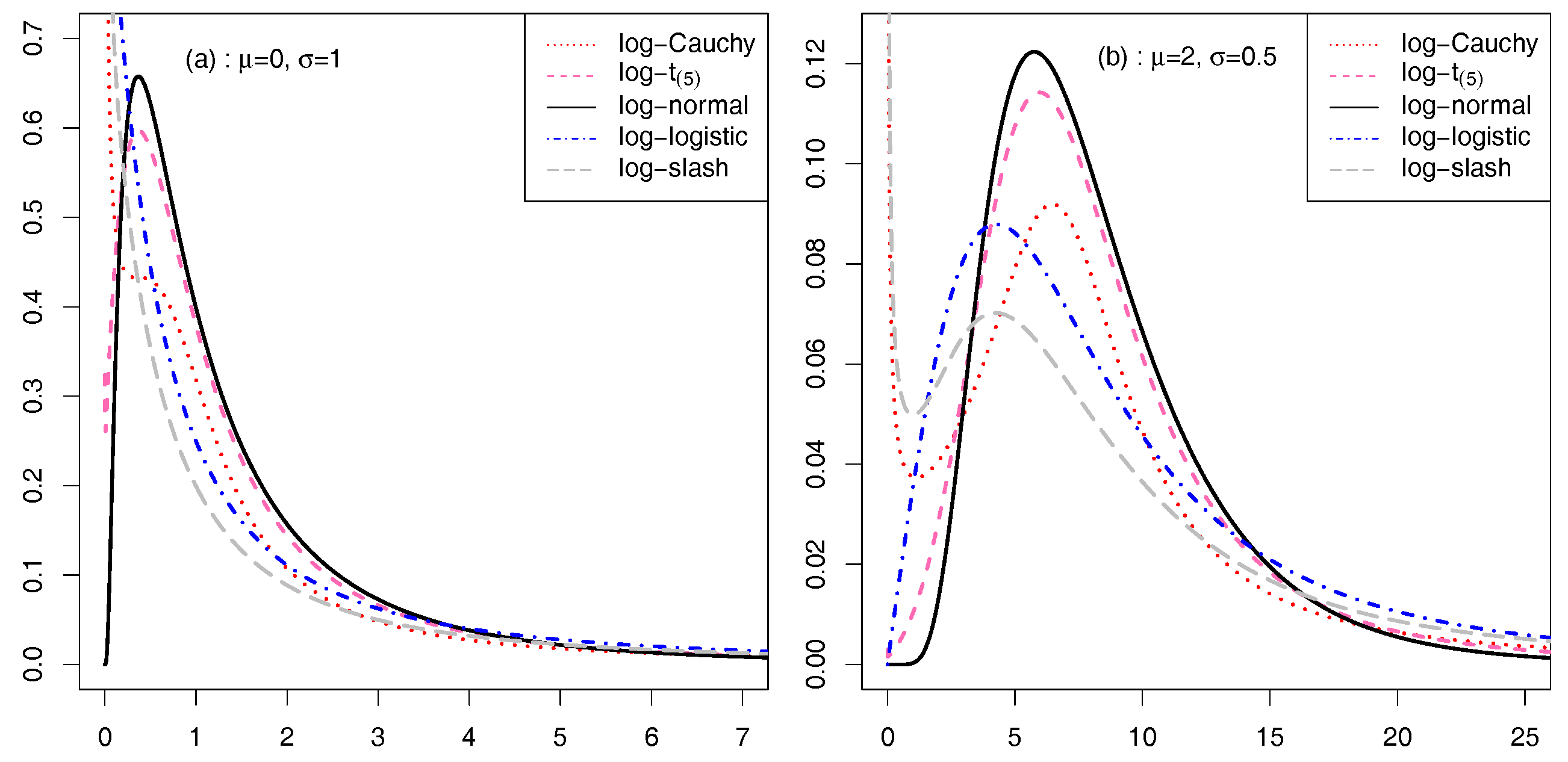
The densities of five class members are shown in Figure 1 for different designations of the mixing distribution and . Figure 1 shows that the tail area of the log-normal density is thinner than that of the other densities. Thus, the use of models is useful for flexible and robust reliability analysis of failure time data involving fat-tailed empirical distribution. Figure 1 also demonstrates that the class of models is useful to describe those situations in which early failure or occurrences dominate the distribution.
Reliability and hazard rate of the class of SMLNFT models are directly related to those of the distribution. Let Y be failure time or down time formulated by the model, and then respective MTTF (mean time to failure) and variance of Y be
In addition, the reliability and hazard rates of the SMLNFT model are given by
and
where and and are the density and the cdf of a standard normal variable, respectively. Exact expressions for Equations (5) and (6) based on the above five FT models are as follows:
- (i)
- LNFT model:where
- (ii)
- LFT model:where and denote the cdf and density function of a Student- distribution, respectively.
- (iii)
- LCFT model:
- (iv)
- LLFT model:
- (v)
- LSFT model:
The reliable life , denoting the 100(1-)th percentile of the failure time distribution of the SMLNFT model, may also be expressed as
The expectations made for the reliability measures (Equation (4) through Equation (7)) are given in respect to the distribution of
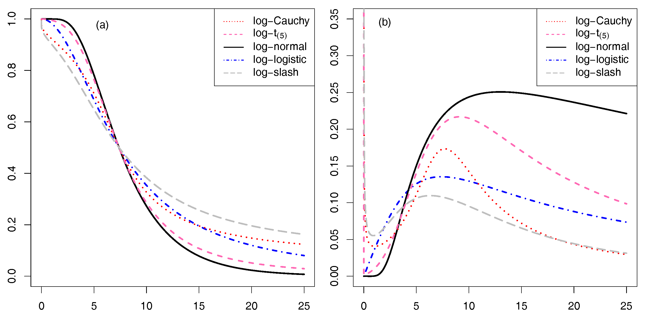
Figure 2 illustrates the reliability and hazard functions for each of five different models (i.e., LNFT, LCFT, LLFT, LFT, and LSFT models) for the choice of and It is apparent from the left panel of Figure 2 that all the reliability functions are monotone decreasing functions of y (time) and approaching zero in relation to sufficiently large values of times, but the shape of the functions are not the same. As expected from the densities of Figure 1, we see that each reliability function of heavy tailed models (i.e., LCFT, LLFT, LFT, and LSFT models) initially decreases more rapidly than that of the LNFT model; then, it decreases toward zero more slowly than that of the LNFT model. The right panel of Figure 2 describes hazard rates of the five models. The hazard rate of the LNFT model initially increases and then decreases toward zero as y (time) passes by. Hazard functions of the LLFT and LFT models resemble that of the LNFT model, aside from a rapid decrease toward zero after the initial increase. However, the right panel shows that the LCFT and LSFT models have different hazard functions from that of the LNFT model in that the initial increase of the hazard rate does not apply to these models.
3. Two-Stage MaxEnt Prior
3.1. Stochastic Constraint on Reliability Measures
Let be n complete (nontruncated/noncensored) failure times generated from the SMLNFT model in Equation (1), and let the reliability measures, defined by Equation (4) through Equation (7), have a stochastic functional constraint in terms of and where the constraint does not depend on Thus, a reliability measure, written by needs to be located in a restricted interval (or equivalently ) with a degree of prior belief where is either an interval or a set of intervals. Nevertheless, observations from the SMLNFT model often do not provide strong evidence that information of the constraint, , is true and therefore may appear to contradict the assumption of the model associated with the constraint.
In this situation, a Bayesian approach can be effectively adopted to model the stochastic (or uncertain) functional constraint on parameter Bayesian reliability analysis of the model (1) begins with specifying prior distribution which represents information concerning the parameters and that are combined with the joint probability distribution of s to yield the posterior distribution:
where is the density given in Equation (3). When there are no constraints on the location parameter , then a common joint prior (e.g., Jeffreys prior or normal-inverse gamma prior) can be used, and posterior reliability inference can be performed without any difficulty. When we have sufficient evidence that the constraint condition on the model (1) is true (i.e., ), then a suitable restriction on the parameter space such as using a truncated prior distribution, e.g., is expected. Here, I denotes an indicator function. See, e.g., [21,22,23,24], for various applications of truncated prior distribution in Bayesian inference. However, it is often the case that prior information about the constraint is not certain to carry out Bayesian reliability analysis. In this case, it is expected that the uncertainty, i.e., is taken into account in eliciting a prior distribution of
3.2. Two-Stage MaxEnt Prior
Assume that is known and that it is possible to specify that partial information concerning the parameter is of the form
but nothing else about prior distribution In this case, maximum entropy prior can be obtained by choosing that maximizes the entropy
in the presence of the partial information in the form of Label (8). Boltzmann’s maximum entropy theorem (see, e.g., [14,15]) tells us that the density that maximizes , subject to the constraints takes the k-parameter exponential family form
where can be determined, via the k-constraints, in terms of …,
The theorem can be directly applied to obtain the MaxEnt prior of the SMLNFT model, provided that prior information on the mean and variance of unconstrained can be specified, i.e., and Supposing that we have additional information that we then have the following lemma.
Lemma 1.
Suppose we can specify partial prior information about μ by and with degree of belief Then, the MaxEnt prior density of μ is given by
where the value of δ ( is determined by the following equation
Here, is probability of , and denotes a joint probability of and whose joint distribution is a bivariate normal
Proof.
The stochastic constraint can be expressed in terms of a moment as Take and for Then, by setting and the MaxEnt prior of in Label (9) reduces to
Now, the second exponential term on the right-hand side of Label (12) can be determined by using the stochastic constraint : among all of the possible proper prior densities of the form (12), the choice of yields a proper prior density. Furthermore, this choice leads to Equation (11), which satisfies the stochastic constraint
☐
From Lemma 1, we see that implies no functional stochastic constraint on of the SMLNFT model, while denotes that the functional constraint on the model is certain so that We also see that reduces to the normal density for the former case and the truncated normal density with the support for the latter case. This indicates that is directly related to the degree of prior belief on the constraint where The relationship between them is as follows.
Corollary 1.
The degree α of prior belief on the constraint accounted for by the MaxEnt prior is and its range is
Proof.
For the cases where and the degree of prior beliefs are and respectively. When
because by the Theorem of [25]. ☐
Corollary 1 indicates that is useful for eliciting priori uncertainty concerning constraint on by varying the value of By applying the work of [26], we can organize within the frame of the two-stage prior hierarchy by [16].
Theorem 1.
The distribution of can be expressed as a two-stage prior hierarchy:
where and denote a truncated distribution with the support
Proof.
From the hierarchy of the prior distributions, we see that
which is equivalent to . ☐
From now on, we shall call the MaxEnt prior expressed by the two-stage prior hierarchy in Theorem 1 as a “two-stage MaxEnt prior” of .
4. Bayesian Hierarchical SMLNFT Model
4.1. Bayesian Hierarchical Model
Let be n complete failure times as generated from the SMLNFT model in Equation (1), and let denote contribution of latent variable in relation to each observation . Suppose one of the reliability measures defined by Equation (4) through Equation (7) has a stochastic functional constraint in terms of e.g., (or equivalently ), with the degree of prior belief and suppose is either an interval or a set of intervals. Then, from Equations (3) and (10), we obtain posterior distribution of and given by
where is a prior distribution of This is a complex function for the Bayesian inference in reliability based on the SMLNFT model. Alternately, following hierarchical representation of the stochastically constrained SMLNFT Model is useful for simple Bayesian inference. Using the two-stage MaxEnt prior in Theorem 1 and assuming prior independence of and we formulate a Bayesian hierarchical model for the stochastically constrained SMLNFT model as follows:
All hyper-parameters, are assumed to be given from the prior information of previous studies or alternate sources. In particular, the value of is chosen to satisfy Equation (11) for given values of and In cases where the prior information is not available, a convenient strategy of avoiding improper posterior distribution is to use proper priors with fixed hyper-parameters as appropriate quantity to reflect the diffuseness of the priors (i.e., limiting non-informative priors).
4.2. The Gibbs Sampler
Let be the latent variables, and let be logarithmic failure time data where Based on the Bayesian Hierarchical SMLNFT model structure, the joint posterior distribution of given the observed data is
where is the density of variate and is the density of the mixing variable Note that the joint posterior distribution of the structure parameters, and is
This is not simplified in an analytic form of known density, and is thus intractable for posterior inference. Accordingly, we treat latent observations in as hypothetical missing data, and augment the observed data set with in posterior analysis. Thus, we derive each conditional posterior distribution of and for posterior inference based on Markov chain Monte Carlo (MCMC). All of the full conditional posterior distributions are as follows:
- (1)
- The full conditional distribution of is an univariate normal given by:where
- (2)
- The full conditional distribution of is a truncated normal given by:where
- (3)
- The full conditional distribution of is a Gamma distribution:
- (4)
- The full conditional distributions of s are independent and their densities arewhere is the density of a mixing variable.
The conditionals in Equation (15) through Equation (18) define the Gibbs sampler, provided that Equation (18) is a known density of standard form. Otherwise, we can define a Metropolis-within-Gibbs sampler that uses an M–H (Metropolis–Hastings) step to sample from the conditional in Equation (18). See [26], for the Metropolis-within-Gibbs sampler.
4.3. Markov Chain Monte Carlo Method
An MCMC method that works with the posterior Equation (14) is not complicated since Gibbs sampling of is routinely implemented based on each of their full conditionals outlined in Section 4.2. However, in posterior sampling of an M–H sampling algorithm may be used when the conditional posterior density Equation (18) does not have explicit form of known distribution. For the MCMC method, one should note the following points.
- note 1:
- With given initial values of , implementation of the Gibbs (or Metropolis-within-Gibbs) sampling algorithm consists of drawing repeatedly from distributions Equation (15) through Equation (18). The R package tmvtnorm and the R package mvtnorm can be used to sample from the conditionals and to calculate for a given from Equation (11).
- note 2:
- In cases using the LNFT model, degenerates at This means that the conditional distribution Equation (18) can be eliminated from the Gibbs sampler by setting for the conditionals of and
- note 3:
- When the LFT model is used for reliability analysis, the last stage of the Bayesian hierarchical model in Equation (13) becomes with Thus, the conditional distribution in Equation (18) yieldswhere denotes an vector whose elements are those of except for Note that the LCFT model is a special case of the LFT model with To allow to be determined within the model, one can specify one more prior stage for the Bayesian hierarchy in Equation (13). As suggested by [19,27], a uniform prior on () can be considered. To limit model complexity, we consider only fixed so that the investigation of different LFT models is possible.
- note 4:
- The conditional distribution Equation (18) for LSFT model isa truncated gamma whose support is
- note 5:
- note 6:
- The convergence of an MCMC algorithm is an important issue for the correct estimation of the posterior distribution of interest. See [30] for an example of multiple convergence diagnosis and output analysis. When the Markov chain is converged, Rao–Blackwellization yields good estimates of and
- note 7:
- As measures of model comparison among SMLNFT models, a deviance information criterion (DIC) can be used. This measure can be calculated based on extensions of the MCMC method. See [31] and references therein for a review and comparisons of such extensions.
The Rao-Blackwellized Bayesian estimate of and from m post-convergence Markov chain values are given by the ergodic theorem as:
As indicated by Equation (4) through Equation (7), it is evident that the reliability measures are functions of and as denoted by Represent Bayesian estimate with
where is joint posterior density of and based on a fitted SMLNFT model, is the density of and is the support of Next, a Bayesian Monte Carlo estimate of is given by
where denote the rth Gibbs sample obtained from a fitted SMLNFT model, while is an independently generated kth sample value from the mixing distribution When we have exact expression of then the Monte Calro integration, using generated s, vanishes from Equation (19). For example, the estimate of posterior predictive reliability of the LFT model for specified y is
where denote the rth Gibbs sample obtained from the fitted LFT model. Now, credible interval of the reliability at time y can be calculated by where denotes the qth quantile value of s with When the LNFT model is assumed, Bayesian estimates of reliability measures can be simply obtained by setting to Equation (18). That is, the reliability at time y is
5. Numerical Illustrations
We provide two data applications to illustrate and demonstrate the performance of the proposed methodology. The first real data application demonstrates the performance of the proposed methodology (MCMC method based on a Bayesian hierarchical SMLNFT model) for inference in reliability with stochastic constraint. Proposed SMLNFT models were fitted to the second data set and compared in terms of their data-fitting performances, estimating parameters, and robustness to fat-tailed empirical distribution. For numerical implementations, we developed our program written in R, which is available from the author upon request.
5.1. Equipment Failure Data Example
This example considers failure time data (assessed in hours) obtained from a reliability study of assembly line equipment in operation in an automobile plant. The data, available in [32], consists of 43 observations of the failure time (Y). It provides summary statistics (mean and standard deviation (S.D.)) as listed in Table 1. We implemented the Shapiro–Wilks (S–W) and Kolmogorov–Smirnov (K–S) tests to determine the log-normality of Y (i.e., normality of ) based on the data. The test statistic values and corresponding p-values are also listed in Table 1.
As seen in the table, the formal tests do not reject the log-normality of i.e., Our objective of data analysis is to estimate reliability measures of the assembly line equipment subject to with , where c and are known values. We can get the prior information about from past studies or an assembly line quality control report. This stochastic constraint on indicates that, with degree of prior belief, the reliability of the LNFT model decreases slower than the empirical implication because Following the proposal of this paper, the two-stage MaxEnt prior can be used to elicit the stochastic constraint on Utilizing we can use the Bayesian hierarchical LNFT model (developed in Section 4) to carry out reliability analysis of the assembly line.
To see the adequacy of the Bayesian hierarchical LNFT model, we fitted the failure time data to five Bayesian hierarchical models (LNFT, LLFT, LCFT, LFT, and LSFT Bayesian hierarchical models) and compared them in terms of deviance information criterion (DIC), which is a measure of model comparison and adequacy. For each of the five models, we set up and ran a MCMC sampling algorithm (using Gibbs sampler) on the failure time data set and generated 100,000 Gibbs samples of model parameters from the conditional posteriors given in Section 4.2. For the MCMC algorithm, we used a burn-in period of 1000, a thin interval of 100, and the following choice of hyper-parameter values: and DIC values of the five models were calculated and they were 132.421, 135.704, 150.209, 135.698, and 145.971 for LNFT, LLFT, LCFT, LFT, and LSFT models, respectively. Thus, Bayesian hierarchical LNFT model achieves minimum DIC value among the five models. This, along with the formal log-normality test results in Table 1, provides support in favor of the LNFT model for fitting the data.
Table 2 shows some posterior summary statistics for the LNFT model. The statistics include posterior estimate, posterior standard deviation (S.D.), 0.025th quantile, 0.975th quantile, and MC error calculated from the Gibbs samples obtained by differing the values of c and Mote Carlo (MC) errors in the table were obtained by setting In estimating the Mote Carlo (MC) errors, we used the batch mean method with 50 batches. See, e.g., ([31], pp. 39–40) for the batch mean method. The degree of the prior belief () in the constraint () were calculated by use of Equation (11), and their values are also listed in Table 2.
The small MC error values listed in Table 2 convince us of the convergence of the MCMC algorithm. The table shows that induces a shrinkage effect in the Bayesian estimation of with the uncertain interval constraint, i.e., This effect can be seen from the comparison of the posterior estimates of obtained from the case of with those from This comparison indicates the followings: (i) the Bayesian estimate of based on the two-stage prior , shrinks toward the interval The magnitude of shrinkage effect induced by using the proposed prior becomes more evident as value of (or the degree of belief in the interval constraint ) gets larger. Especially, in the case of and we see that the 95% credible interval for does not include (estimate of with no constraint). This highlights the shrinkage effect induced by using (ii) When the priori constraint is certain, i.e., Table 2 shows that estimate of is located in the given constraint This advocates the use of the Bayesian hierarchical LNFT model for reflecting the uncertain parameter constraint in reliability analysis.
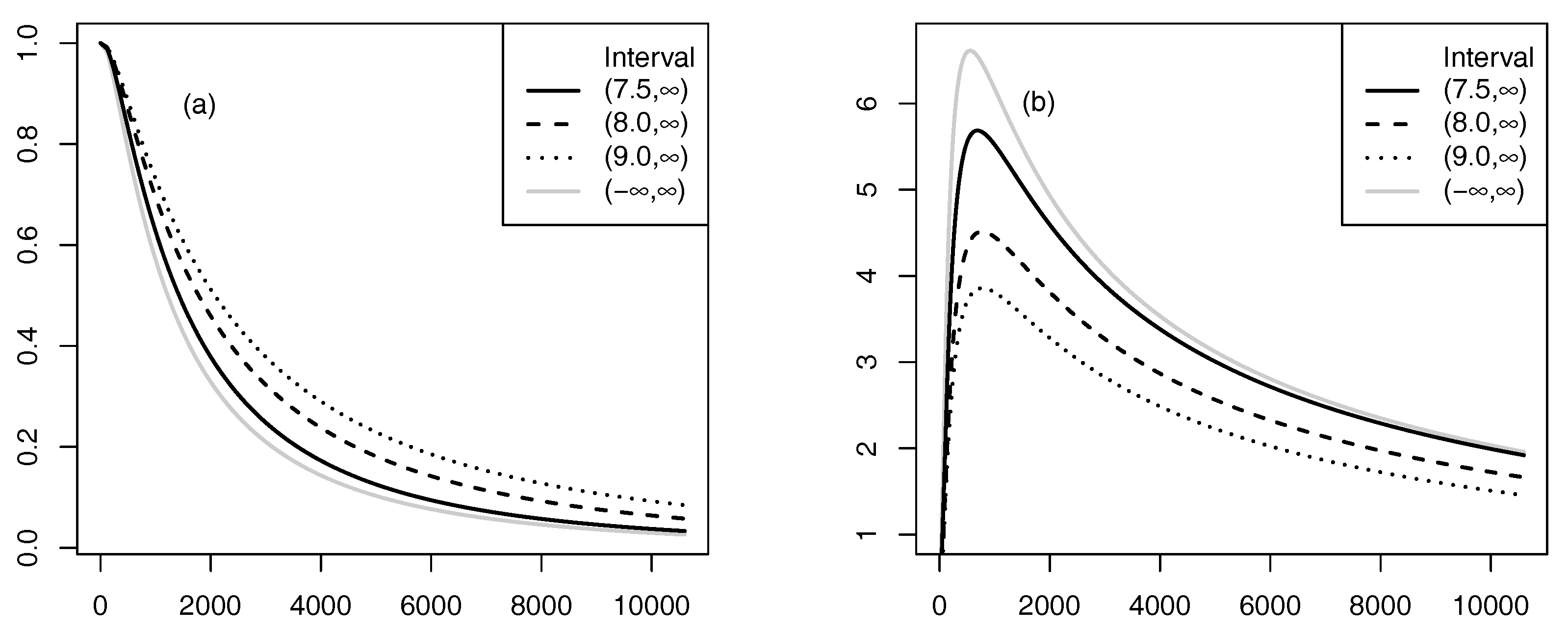
Posterior predictive reliability measures of the LNFT model were also estimated by using the failure time data. Figure 3 depicts estimates of posterior predictive reliability and hazard rate functions for each case where the stochastic constraint is for given The figure also compares the functions with those obtained by setting , which denotes the case where there is no priori constraint on , i.e., the case of Figure 3 clearly indicates that the two-stage MaxEnt prior appropriately reflects the priori stochastic constraint in estimating the posterior predictive predictive measures. The left panel (a) shows that reliability of the constrained LNFT model decreases slower than that of the unconstrained model (with ), and this phenomenon is more evident as the constrained interval locates far from the empirical mean value This, in turn, affects shape of hazard rate functions in the right panel (b). For priori constrained LNFT models tend to produce lower hazard rates than the unconstrained LNFT model at all time points, but the pattern of their hazard rate functions is similar. We also see that the hazard rate becomes lower as the value of c gets larger. This coincides with the implication of the reliability functions in the panel (a).
5.2. Artificial Data Example
A study using artificial data is done to evaluate the performance of proposed Bayesian hierarchical estimation methodology based on the class of SMLNFT models. For the study, we have considered a LFT model with location and scale parameter By use of the model, we simulated a sample of size 300 in complete failure times. Five models (LNFT, LCFT, LFT, LSFT, and LLFT models) were fitted to the same simulated data. Using the data, we ran the MCMC sampling algorithm based on each Bayesian hierarchical model with no constraint (i.e., ) and generated 50,000 random samples from the conditional posteriors by using a burn-in period of 5000 and a thin interval of 10. For constructing each hierarchical model, we used the following choice of hyper-parameter values, and which reflect the diffuseness of the priors (i.e., limiting non-informative priors) of and
Table 3 provides posterior summaries from the posterior samples generated by using the MCMC algorithm developed for each of the five models. The small MC error values listed in Table 3 indicate that we have calculated the parameter estimates with precision and the MCMC algorithm has converged to its target distributions as well. DIC values of all models are also presented in the table. We observe that the LFT model has the lower DIC value, while the other models’ results are considerably higher DIC values than the corresponding one under the LFT model. This demonstrates model selection function of the methodology. Concerning the posterior estimates, the estimate of under the LFT model is accurate in comparison to that under the other models. To be more specific, the scale parameter ranges from 0.025 to 0.365 with 95% posterior probability for the LFT model, while, for the other models, none of the credible intervals include true value with the same posterior probability. On the other hand, Table 3 shows that the MCMC algorithm applied to each of the five models correctly estimates true location parameter value This implies that the proposed LFT model is robust to fat tailed failure time observations affecting the scale parameter.
6. Conclusions
This paper has provided a methodology for Bayesian inference in reliability of SMLNFT models in cases where the interval constraint must be incorporated due to uncertainty. For failure time modeling with stochastic restriction, we proposed a Bayesian hierarchical model involving a two-stage MaxEnt prior distribution of based on Boltzmann’s maximum entropy theorem. The two-stage MaxEnt prior reflects uncertainty about the prior constraint, that is, the Bayesian hierarchical SMLNFT models are subject to reliability restriction with uncertainty. Furthermore, we provide an MCMC method for assessing inference in the reliability of SMLNFT models based on their Bayesian hierarchical models. The effectiveness of our methodology is demonstrated by conducting two data applications.
We find that the proposed class of SMLNFT models is flexible enough to account for the behavior of reliability, unlike the log-normal FT model. We also find a connection between the degree of constraint presumption and the hyper-parameters of the two-stage MaxEnt prior, indicating adequacy of the MaxEnt prior in eliciting the priori uncertain constraint (see Corollary 1). Finally, we find that the proposed Bayesian hierarchical methodology enables the development of a simple MCMC algorithm to assess the posterior inference in reliability of the SMLNFT models with a stochastic constraint. Our proposed methodology can be easily extended to cases where the failure time data is incomplete, as a result, for example, of truncated or censored data, as well as to other FT models, including exponential, Weibull, and Gamma FT models. In addition, the class of SMLNFT models could accommodate multivariate FT models at higher dimension without much difficulty. The methodological process proposed here in relation to Bayesian estimation can be extended to the multivariate models with a multivariate stochastic constraint.
Acknowledgments
The research of Hea-Jung Kim was supported by a Basic Science Research Program through the National Research Foundation of Korea (NRF) funded by the Ministry of Education (NRF-2015R1D1A1A01057106).
Conflicts of Interest
The author declares no conflict of interest.
References
- Stefanescu, C.; Turnbull, B.W. Multivariate frailty models for exchangeable survival data with covariates. Technometrics 2006, 48, 411–417. [Google Scholar] [CrossRef]
- Kavam, P.H.; Pena, E.A. Estimating load-sharing properties in a dynamic reliability system. J. Am. Stat. Assoc. 2005, 100, 262–272. [Google Scholar] [CrossRef]
- Sun, J. The Statistical Analysis of Interval-Censored Failure Time Data; Spring: New York, NY, USA, 2002. [Google Scholar]
- Yue, S. The bivariate lognormal distribution for describing joint statistical properties of multivariate storm event. Environmetrics 2002, 13, 811–819. [Google Scholar] [CrossRef]
- Yerel, S.; Konuk, A. Bivariate lognormal distribution model of cutoff grade impurities: A case study of magnesitr ore deposit. Sci. Res. Essay 2009, 4, 1500–1504. [Google Scholar]
- Lee, C.-F.; Finnerty, J.; Lee, J.; Lee, A.C.; Wort, D. Security Analysis, Portpolio Management, and Financial Derivatives; World Scientific Publishing Company: Singapore, 2012. [Google Scholar]
- Halliwell, L.J. The lognormal random multivariate. In Casualty Actuarial Society E-Forum; Spring, 2015; Available online: www.casact.org/pubs/forrum/15spforum/Halliwell.pdf (accessed on 13 June 2017).
- Weinke, A. Frailty Models in Survival Analysis; Chapman and Hall: Baco Raton, FL, USA, 2010. [Google Scholar]
- De Alba, E. Claims reserving when there iare negative values in the runoff triangle: Bayesian analysis using the three-parameter log-normal distribution. N. Am. Axtuarial J. 2006, 10, 28–38. [Google Scholar]
- Yue, S. The bivariate lognormal distribution to model a multivariate flood episode. Hydrol. Process. 2000, 14, 2575–2588. [Google Scholar] [CrossRef]
- Elshqeirat, B.; Soh, S.; Rai, S.; Lazarescu, M. Dynamic programming for minimal cost topology with reliability constraint. J. Adv. Comput. Netw. 2013, 1, 286–290. [Google Scholar] [CrossRef]
- Lin, Y.-K. Reliability evaluation for an information network with node failure under cost constraint. IEEE Trans. Syst. Man Cybern. Part A Syst. Hum. 2007, 37, 180–188. [Google Scholar] [CrossRef]
- Koide, T.; Shinmori, S.; Ishii, H. Topological optimization with a network reliability constraint. Discret. Appl. Math. 2001, 115, 135–149. [Google Scholar] [CrossRef]
- Cercignani, C. The Boltzman Equation and Its Applications; Springer: Berlin, Germany, 1988. [Google Scholar]
- Leonard, T.; Hsu, J.S.J. Bayesian Methods: An Analysis for Statisticians and Interdisciplinary Researchers; Cambridge University Press: Cambridge, UK, 1999. [Google Scholar]
- O’Hagan, A.; Leonard, T. Bayes estimation subject to uncertainty about parameter constraints. Biometrika 1976, 63, 201–203. [Google Scholar] [CrossRef]
- Lachos, V.H.; Labra, F.V.; Bolfarine, H.; Ghosh, P. Multivariate measurement error models based on scale mixtures of the skew-normal distribution. Statistics 2010, 44, 541–556. [Google Scholar] [CrossRef]
- Lindsey, J.K. Statistical Analysis of Stochastic Process in Time; Cambridge University Press: Cambridge, UK, 2004. [Google Scholar]
- Chen, M.H.; Dey, D.K. Bayesian modeling of correlated binary responses via scale mixture of multivariate normal link functions. Sankhya´ Indian J. Stat. 1998, 60, 322–343. [Google Scholar]
- Gago-Benitez, A.; Fernádo-Madrigal, J.-A.; Cruz-Martin, A. Log-logistic modeling of sensory flow delays in networked telerobots. IEEE Sens. J. 2013, 13, 2294–2953. [Google Scholar] [CrossRef]
- Kim, H.J. A best linear threshold classification with scale mixture of skew normal populations. Comput. Stat. 2015, 30, 1–28. [Google Scholar] [CrossRef]
- Steiger, J. When constraints interact: A caution about reference variables, identification constraints, and scale dependencies in structural equation modeling. Psychol. Methods 2002, 7, 210–227. [Google Scholar] [CrossRef] [PubMed]
- Lopes, H.F.; West, M. Bayesian model assessment in factor analysis. Stat. Sin. 2004, 14, 41–67. [Google Scholar]
- Loken, E. Identification constraints and inference in factor models. Struct. Equ. Model. 2005, 12, 232–244. [Google Scholar] [CrossRef]
- Gupta, S.D. A note on some inequalities for multivariate distribution. Bull. Calcutta Stat. Assoc. 1969, 18, 179–180. [Google Scholar] [CrossRef]
- Kim, H.J. A two-stage maximum entropy prior of location parameter with a stochastic multivariate interval constraint and its properties. Entropy 2016, 18, 1–20. [Google Scholar] [CrossRef]
- Sisson, S. Trans-dimensional Markov chains: A decade of progress and future perspectives. J. Am. Stat. Assoc. 2005, 100, 1077–1089. [Google Scholar] [CrossRef]
- Koop, G; Poirier, D.J.; Tobias, J.L. Bayesian Econometric Methods; Cambridge University Press: Cambridge, UK, 2007. [Google Scholar]
- Chib, S.; Greenberg, E. Understanding the Metropolis-Hastings algorithm. Am. Stat. 1995, 49, 327–335. [Google Scholar] [CrossRef]
- Heidelberger, P.; Welch, P. Simulation run length control in the presence of an initial transient. Oper. Res. 1992, 31, 1109–1144. [Google Scholar] [CrossRef]
- Ntzoufras, I. Bayesian Modeling Using WinBUGS; Wiley: New York, NY, USA, 2009. [Google Scholar]
- Dagpunar, J.S. Simulation and Monte Carlo; Wiley: New York, NY, USA, 2007. [Google Scholar]
Figure 1.
Densities of for five different choices of the mixing variable distribution and : (a) case and (b) case.
Figure 1.
Densities of for five different choices of the mixing variable distribution and : (a) case and (b) case.

Figure 2.
Reliability and hazard functions for five models with : (a) reliability functions, ; (b) hazard functions, .
Figure 2.
Reliability and hazard functions for five models with : (a) reliability functions, ; (b) hazard functions, .

Figure 3.
Estimated posterior predictive reliability measures for : the label for the y-axis of (a) is reliability and that of (b) is hazard rate. The label for the x-axis is failure time and the value for tick marks in the y-axis of (b) is multiplied by .
Figure 3.
Estimated posterior predictive reliability measures for : the label for the y-axis of (a) is reliability and that of (b) is hazard rate. The label for the x-axis is failure time and the value for tick marks in the y-axis of (b) is multiplied by .


Table 1.
Summary statistics for the failure time data.
| Variable | Mean | S.D. | S–W (p-Value) | K–S (p-Value) |
|---|---|---|---|---|
| Y | 2201.488 | 2519.174 | 0.732 (<0.01) | 0.231 (<0.01) |
| X | 7.143 | 1.088 | 0.982 (0.760) | 0.064 (>0.150) |
Table 2.
Posterior summaries for each model parameters and degree of prior belief.
| Parameter | S.D. | 2.5% | 97.5% | MC Error | |||||
|---|---|---|---|---|---|---|---|---|---|
| 7.141 | 7.182 | 7.261 | 7.553 | 0.155 | 6.964 | 7.569 | 0.002 | ||
| 1.181 | 1.185 | 1.196 | 1.327 | 0.295 | 0.812 | 1.930 | 0.004 | ||
| 0.308 | 0.698 | 0.865 | 1.000 | - | - | - | - | ||
| 7.141 | 7.202 | 7.364 | 8.029 | 0.157 | 7.067 | 7.684 | 0.002 | ||
| 1.181 | 1.188 | 1.228 | 1.941 | 0.313 | 0.823 | 2.036 | 0.004 | ||
| 0.158 | 0.660 | 0.834 | 1.000 | - | - | - | - | ||
| 7.141 | 7.255 | 7.637 | 9.035 | 0.187 | 7.306 | 8.041 | 0.002 | ||
| 1.181 | 1.198 | 1.408 | 4.734 | 0.401 | 0.901 | 2.450 | 0.005 | ||
| 0.023 | 0.610 | 0.780 | 1.000 | - | - | - | - |
Table 3.
Posterior summaries for parameters of five models.
| Model | Parameter | Mean | S.D. | MC Error | 2.5% | Median | 97.5% | DIC |
|---|---|---|---|---|---|---|---|---|
| LNFT | 2.043 | 0.147 | <0.001 | 1.755 | 2.043 | 2.332 | 861.602 | |
| 4.329 | 0.438 | 0.002 | 3.554 | 4.300 | 5.274 | - | ||
| LCFT | 1.948 | 0.043 | <0.001 | 1.863 | 1.948 | 2.035 | 463.242 | |
| 0.146 | 0.026 | <0.001 | 0.101 | 0.146 | 0.204 | - | ||
| LFT | 1.948 | 0.043 | <0.001 | 1.862 | 1.948 | 2.033 | 394.339 | |
| 0.289 | 0.036 | <0.001 | 0.225 | 0.286 | 0.365 | - | ||
| LSFT | 1.992 | 0.118 | <0.001 | 1.761 | 1.992 | 2.227 | 867.325 | |
| 0.557 | 0.098 | <0.001 | 0.389 | 0.548 | 0.776 | - | ||
| LLFT | 2.025 | 0.132 | <0.001 | 1.767 | 2.025 | 2.282 | 842.847 | |
| 1.363 | 0.176 | <0.001 | 1.056 | 1.350 | 1.745 | - |
© 2017 by the author. Licensee MDPI, Basel, Switzerland. This article is an open access article distributed under the terms and conditions of the Creative Commons Attribution (CC BY) license (http://creativecommons.org/licenses/by/4.0/).
Share and Cite
MDPI and ACS Style
Kim, H.-J. Bayesian Hierarchical Scale Mixtures of Log-Normal Models for Inference in Reliability with Stochastic Constraint. Entropy 2017, 19, 274. https://doi.org/10.3390/e19060274
AMA Style
Kim H-J. Bayesian Hierarchical Scale Mixtures of Log-Normal Models for Inference in Reliability with Stochastic Constraint. Entropy. 2017; 19(6):274. https://doi.org/10.3390/e19060274
Chicago/Turabian StyleKim, Hea-Jung. 2017. "Bayesian Hierarchical Scale Mixtures of Log-Normal Models for Inference in Reliability with Stochastic Constraint" Entropy 19, no. 6: 274. https://doi.org/10.3390/e19060274
Note that from the first issue of 2016, this journal uses article numbers instead of page numbers. See further details here.