Non-Linear Stability Analysis of Real Signals from Nuclear Power Plants (Boiling Water Reactors) Based on Noise Assisted Empirical Mode Decomposition Variants and the Shannon Entropy


Abstract
:1. Introduction
- Study the stability margins of the plant under normal operating conditions and in unusual conditions.
- Predict reactor transients in an event of instability.
- Develop measures to prevent and mitigate the consequences of an event of instability.
2. BWRs Background
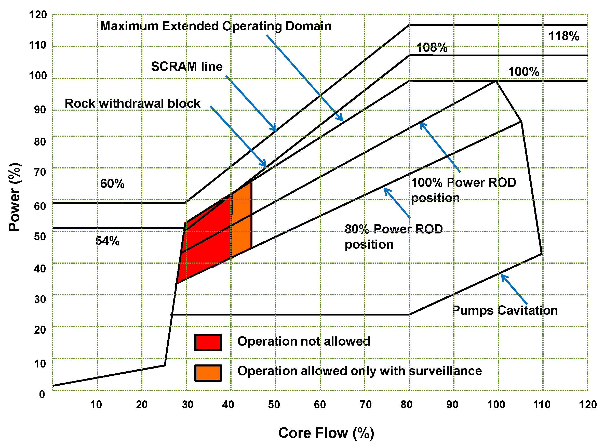
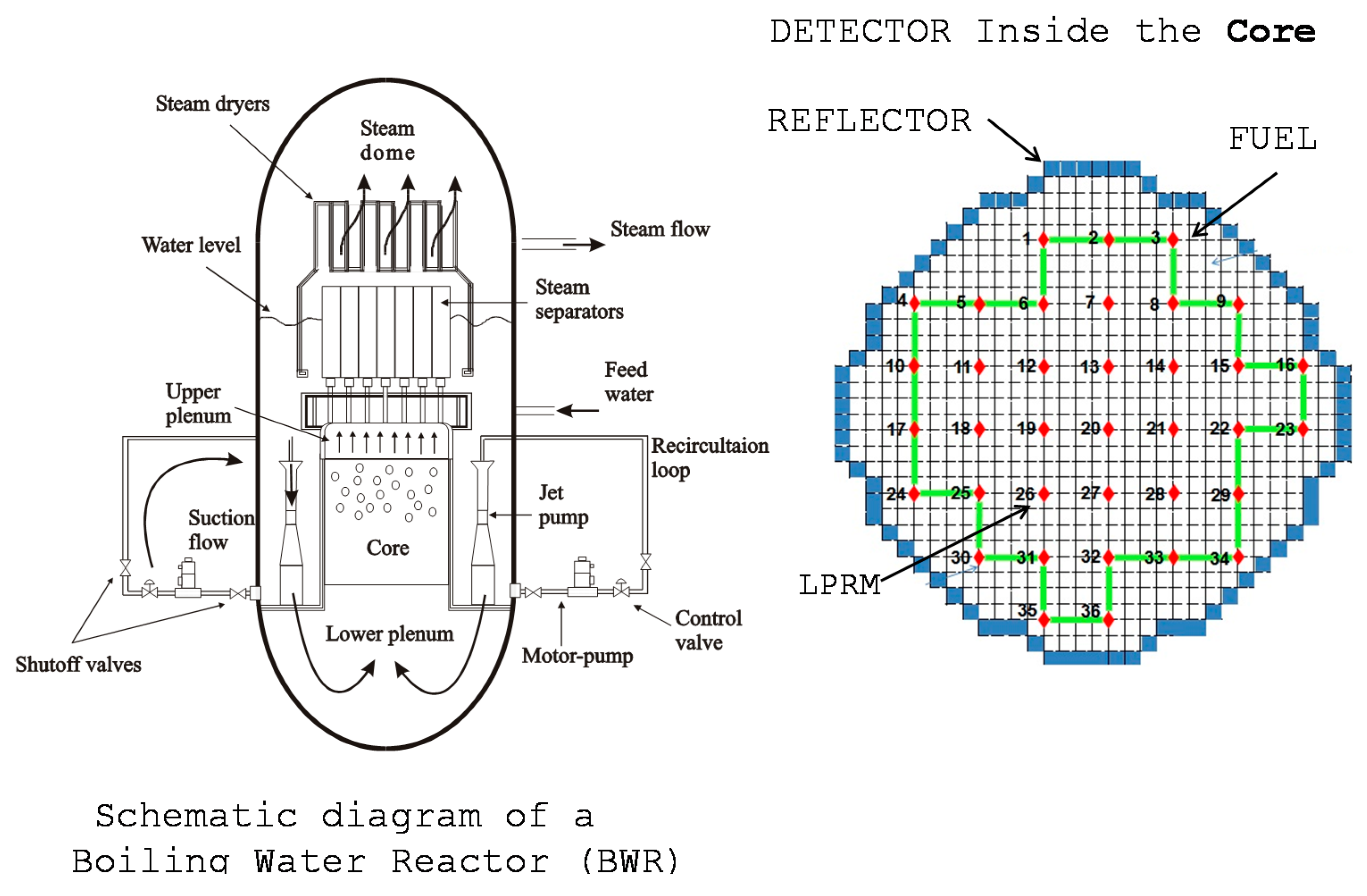
2.1. Description of a BWR
2.2. Instrumentation Inside the Core of a BWR
3. Empirical Mode Decomposition (EMD) Algorithms
3.1. The Default EMD Method
- (I)
- The number of extrema (maxima and minima) and the number of zero-crossings must be equal or differ at most by one.
- (II)
- The local mean, defined as the mean of the upper and lower envelopes, must be zero.
- Step 1.
- Set and find all extrema of .
- Step 2.
- Interpolate between minima (maxima) of to obtain the lower (upper) envelope .
- Step 3.
- Compute the mean envelope .
- Step 4.
- Compute the IMF candidate .
- Step 5.
- Is an IMF?
- Yes. Save , compute the residue , do , and treat as input data in step 2.
- No. Treat as input data in step 2.
- Step 6.
- Continue until the final residue satisfies some predefined stopping criterion.
3.2. The Improved Complete Ensemble Empirical Mode Decomposition Method with Assisted Noise (iCEEMDAN)
- (i)
- Let be the operator which produces the local mean (the mean envelope of the upper and lower envelopes of the studied signal interpolated by cubic splines) of the signal it is applied to.
- (ii)
- Let be the action of averaging throughout an ensemble of realizations of default EMD.
- (iii)
- Let be the operator that produces the k-th mode obtained by default EMD.
- Step 1.
- Calculate by default EMD the local means of I realizations to obtain the first residue:
- Step 2.
- At the first stage (k = 1) calculate the first mode:
- Step 3.
- Estimate the second residue as the average of local means of the realizations and define the second mode:
- Step 4.
- For calculate the k-th residue:
- Step 5.
- Compute the k-th mode:
- Step 6.
- Go to Step 4 for next k.
3.3. The Noise Assisted Multivariate Empirical Mode Decomposition (NA-MEMD)
- Step 1.
- Step 2.
- Calculate a projection, denoted by , of the input multivariate signal along the direction vector , for all k (the whole set of direction vectors), giving as the set of projections.
- Step 3.
- Find the time instants corresponding to the maxima of the set of projected signals .
- Step 4.
- Interpolate , for all values of k, to obtain multivariate envelope curves .
- Step 5.
- For a set of K direction vectors, calculate the mean of the envelope curves as
- Step 6.
- Extract the detail using . If the detail fulfills the stoppage criterion [30] for a multivariate IMF, apply the above procedure to , otherwise apply it to .
- Step 1.
- Create an uncorrelated Gaussian white noise time-series (m-channel) of the same length as that of the input.
- Step 2.
- Add the noise channels (m-channels) created in step 1 to the input multivariate (N-channels) signal, obtaining an (N + m)-channel signal.
- Step 3.
- Process the resulting (N + m)-channel multivariate signal using the MEMD algorithm (listed above), to obtain multivariate IMFs.
- Step 4.
- From the resulting (N + m)-variate IMFs, discard the m channels corresponding to the noise, giving a set of N-channel IMFs corresponding to the original signal.
4. The Shannon Entropy as Stability Indicator
- (i)
- Parametrizing it.
- (ii)
- Dropping the most unlikely values.
- (iii)
- Assuming some a priori shape for the probability distribution.
5. Methodology Based on Shannon Entropy
5.1. Methodology 1: Stability Monitor Based on the iCEEMDAN and the SE
- Step 1.
- The considered signal (APRM or LPRM) obtained from the BWR is segmented in windows of 15 s of duration.
- Step 2.
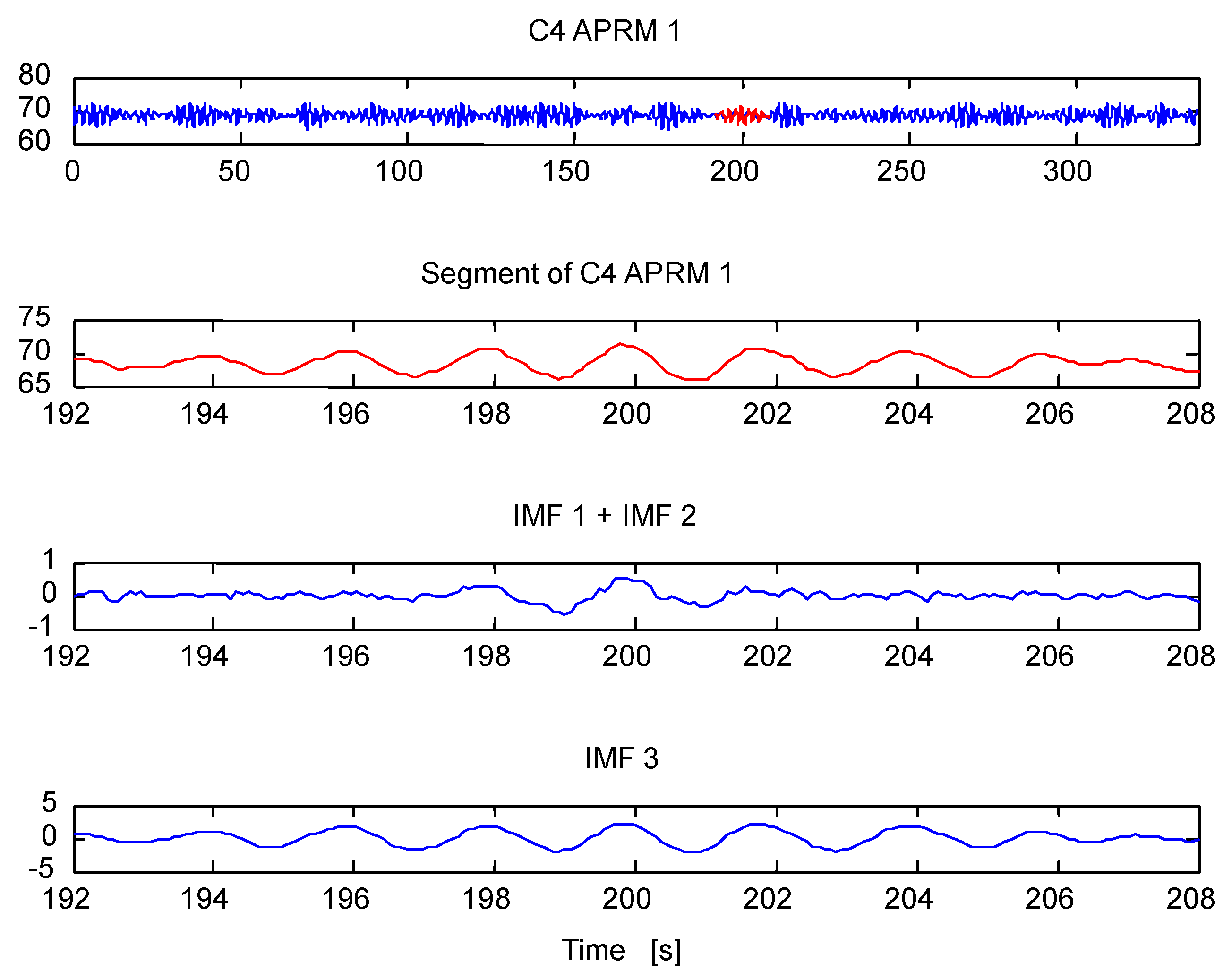
- Each segmented signal (APRM or LPRM) is studied (decomposed) using the iCEEMDAN method for a number of realizations of the ensemble I = 100 and standard deviation of the assisted noise , described above, obtaining in this way the corresponding IMFs. It is worth mentioning that the APRM or LPRM signals are not being processed before. For instance, to remove the signal trend, due that this information is contained in the residue of the decomposition.
- Step 3.
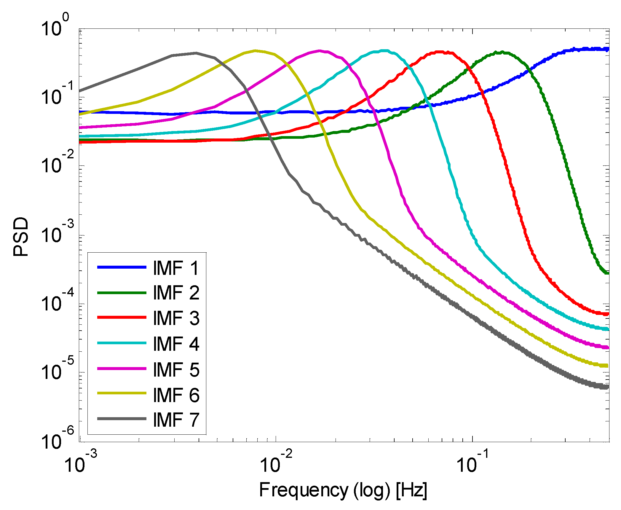
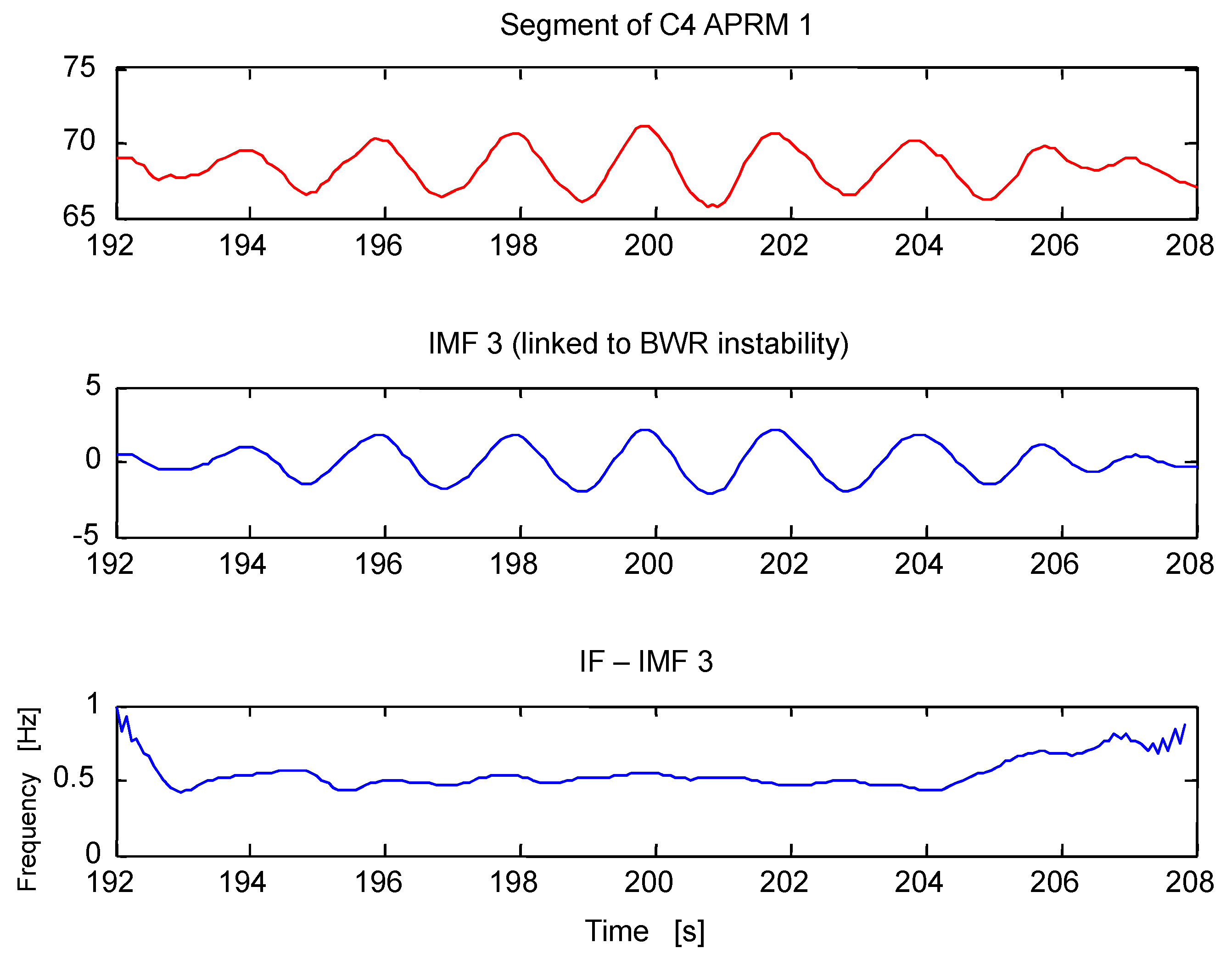
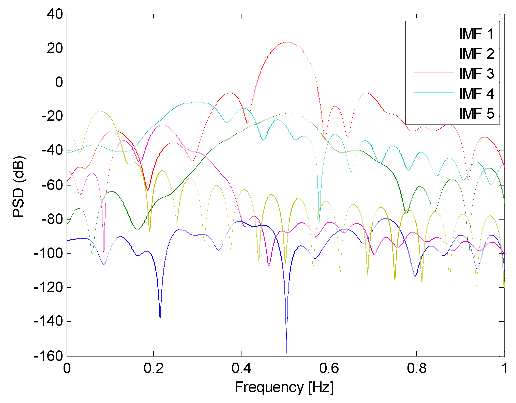
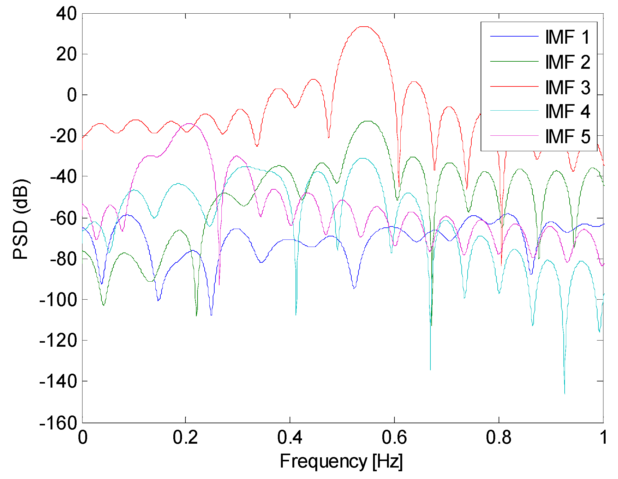
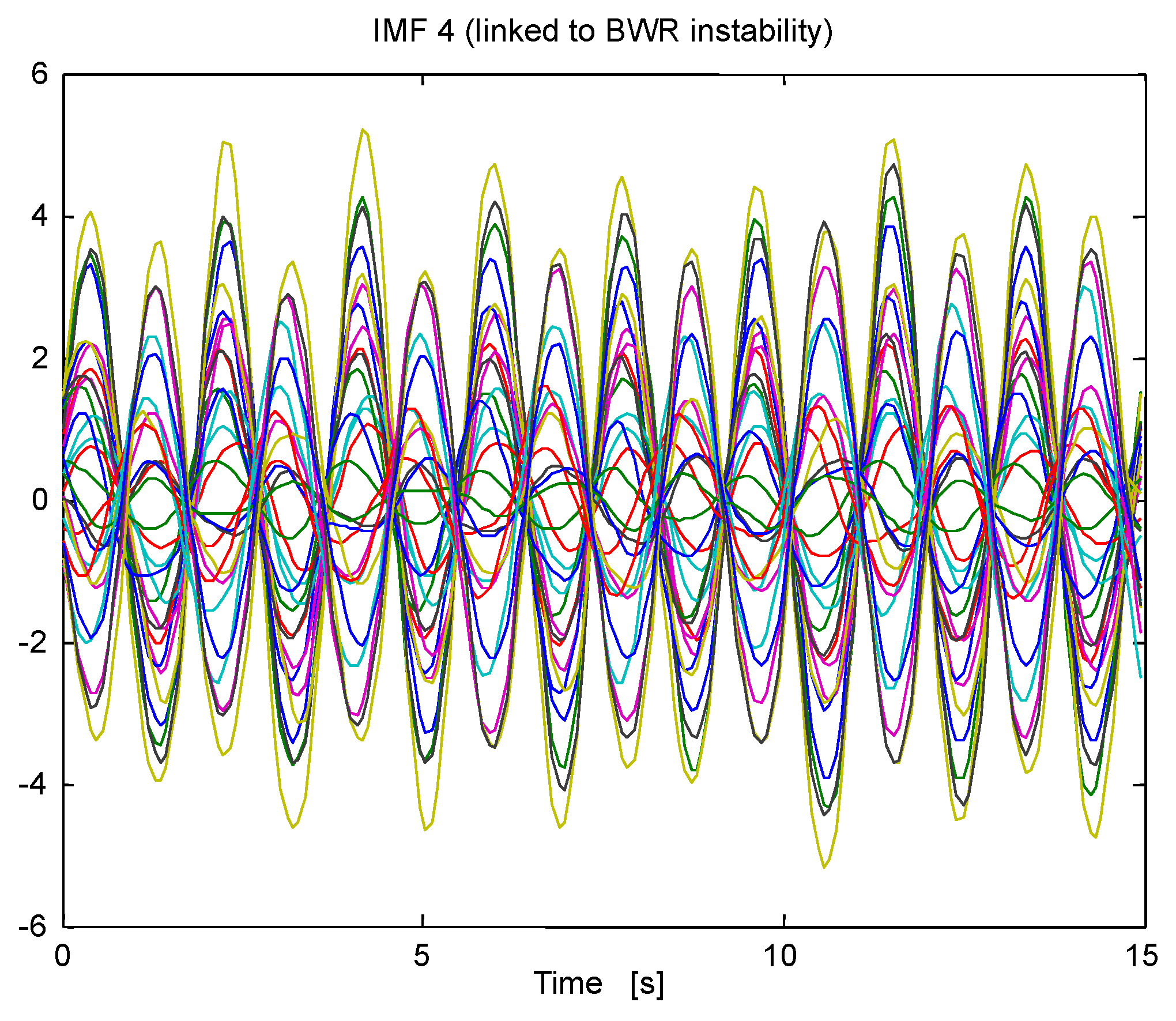
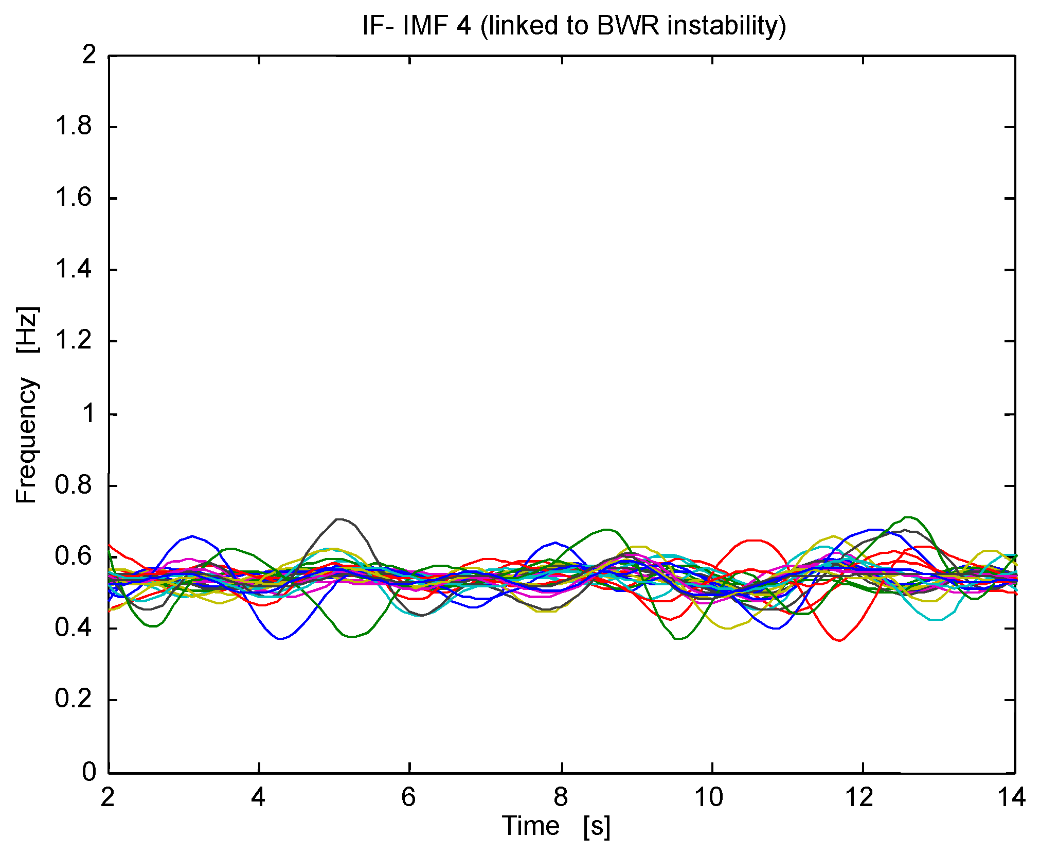
- The Hilbert transform of each IMF is computed in order to get the instantaneous frequencies contained in each IMF (this step is also known as Hilbert Huang transform, HHT, [17]).
- Step 4.
- When tracking these frequencies, it is possible to get the mode linked to instability processes. In this regard, only the IMF associated to BWR instability is considered for further processing.
- Step 5.
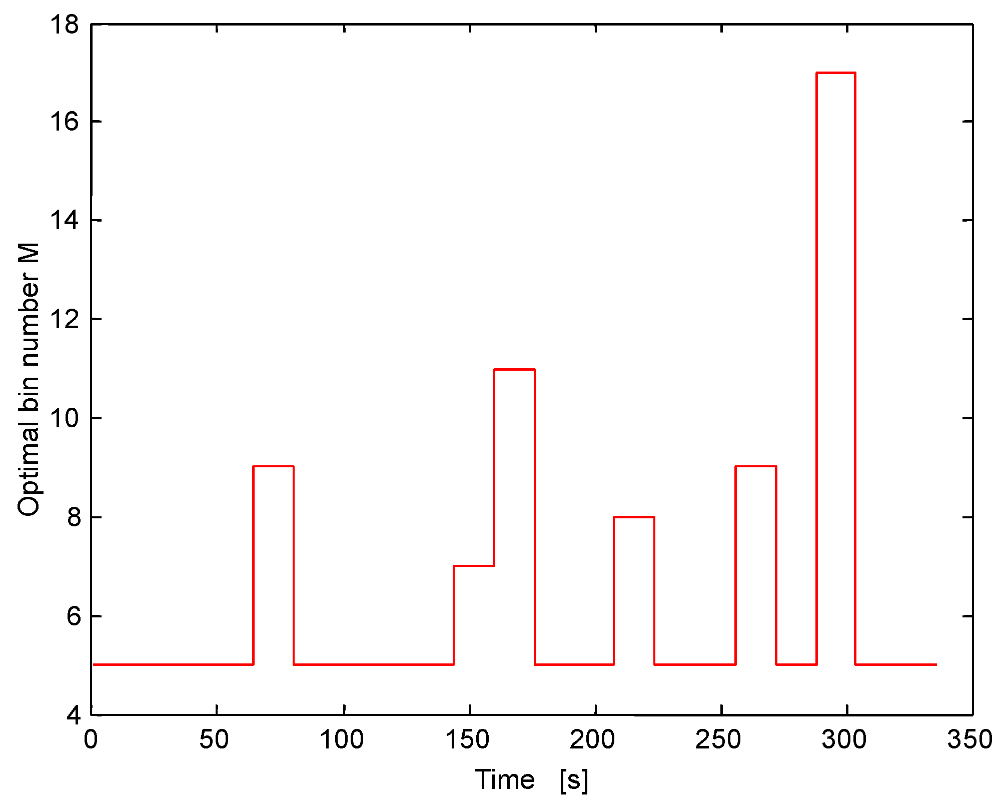
- The SE of the tracked IMF (mode of interest linked to BWR instability) is computed considering the estimator given in Equation (3), using the probability estimator given in Equation (2). The optimal number of bins M for the histogram, is calculated with a technique based on the Bayesian probability theory [32], within the interval (Several rules of thumb exist for determining the number of bins, such as the belief that between 5–20 bins is usually adequate [32]).
- Step 6.
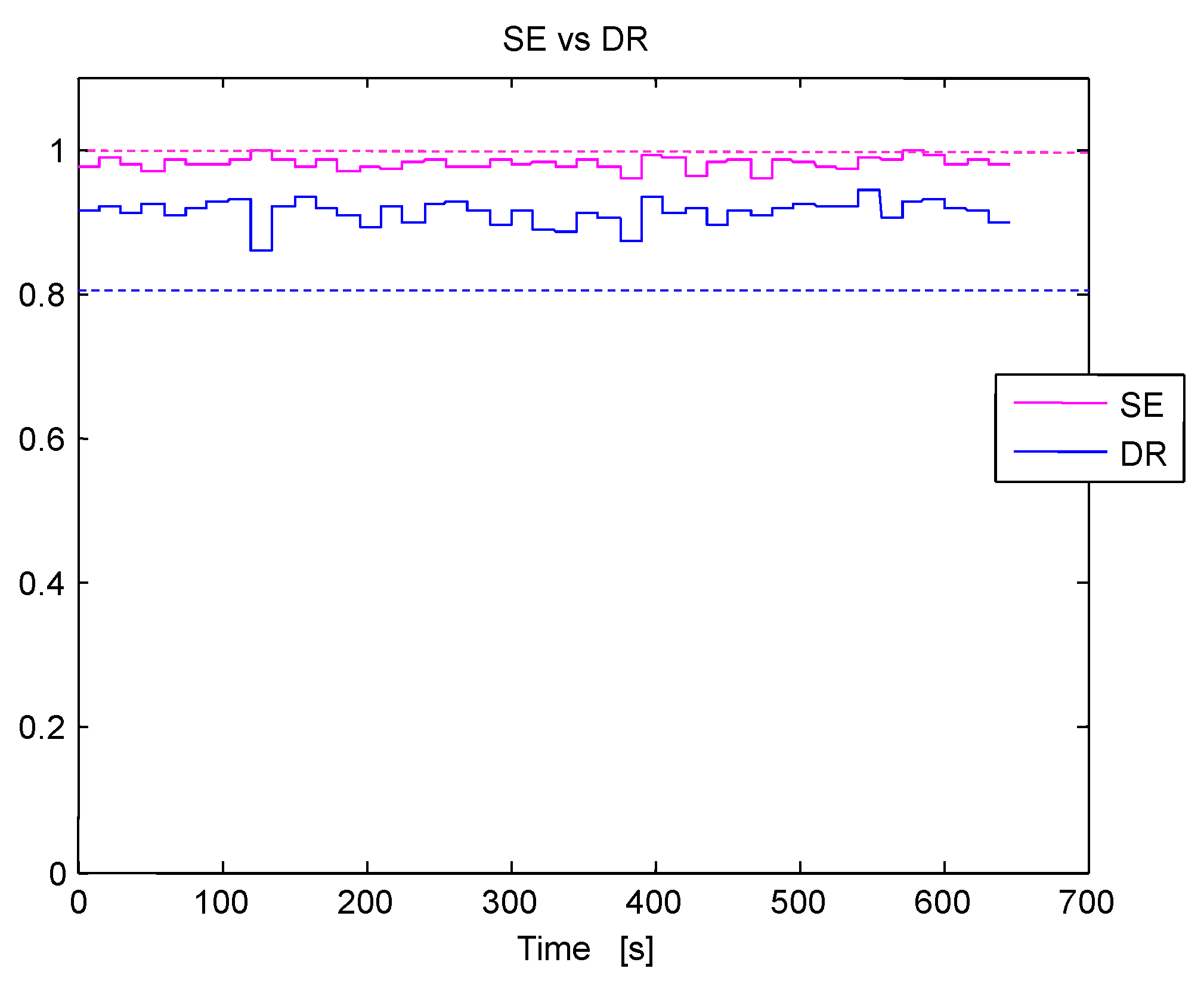
- The mean and variance of the SE are calculated and averaged along all the studied segments of 15 s.
- Step 7.
- In order to range the SE between 0 and 1, the following normalization process is applied:
5.2. Methodology 2: Stability Monitor Based on the NA-MEMD and the SE
- Step 1.
- The considered multivariate signal (an array of N independent LPRM signals) obtained from the BWR are segmented in small windows of 15 s.
- Step 2.
- These segments (of 15 s each of time span) are decomposed in parallel through NA-MEMD in N independent channels. Also, m independent channels of white Gaussian noise are added (to mitigate the mode mixing problem) for decomposition (m = 3 for all of our computer simulations).
- Step 3.
- After decomposition, discard the m channels corresponding to the noise, giving a set of N-channel IMFs corresponding to the original signal segments.
- Step 4.
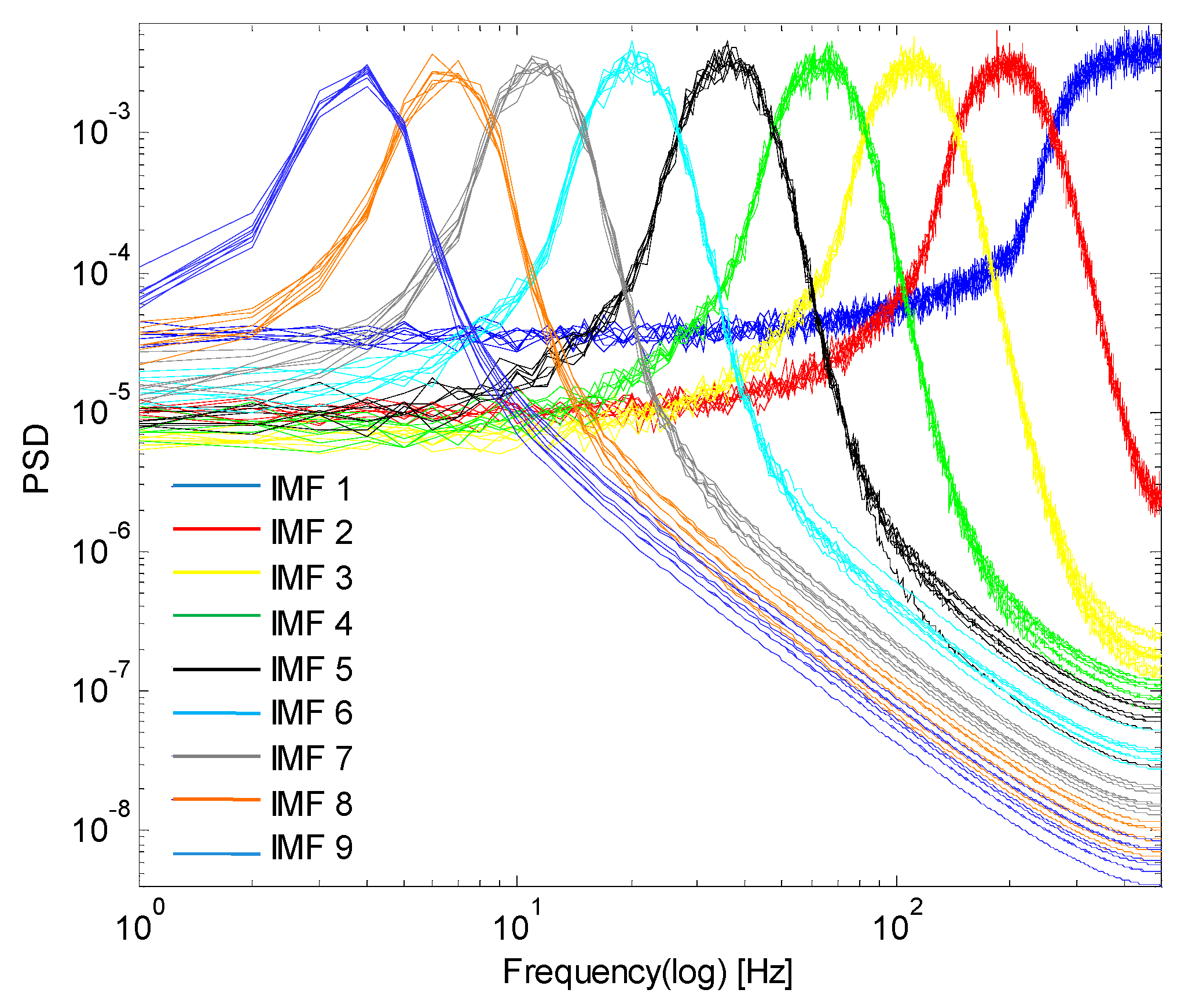
- The Hilbert transform of each IMF is computed in order to get the instantaneous frequencies contained in each N -channel IMFs frequencies (i.e., the HHT).
- Step 5.
- When tracking these frequencies, it is possible to get the IMFs (or modes) linked to instability processes. In this regard, only the IMFs associated to BWR instability are considered for further processing. Exploiting the NA-MEMD properties, the chosen IMFs of interest are all located at the same level of decomposition.
- Step 6.
- The SE of the tracked IMFs (modes of interest linked to BWR instability) are computed via Equation (3). The optimal number of bins M for the histogram, is calculated with the method given in [32] in a local way, within the interval 5 ≤ M ≤ 20. There are thus, N different values of SE (each SE value is linked to one LPRM in particular).
- Step 7.
- The mean and variance of the SE values are calculated and averaged along all the studied multivariate segments of 15 s.
- Step 8.
- In order to range the SE estimates between 0 and 1, the normalization procedure given in Equation (4) is again applied.
6. Results: Methodologies Performances and Discussions
6.1. Stability Analysis of the Chosen Real Cases Through the Methodology 1
- (I)
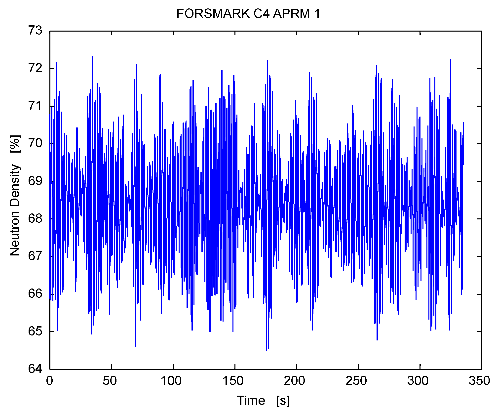
- Case 4 of the Forsmark stability benchmark. This event is considered a challenging case to be analyzed by the complexity of the phenomenon. For reasons of space, only this challenging case is presented in a detailed way. The studied Case 4 contains a mixture between a global oscillation mode and a regional (half core) oscillation. This event corresponds to a situation where the neutronic power reactor suffers abnormal and apparently unstable oscillations. The C4_APRM and C4_LPRM_x signals correspond to average power range monitor (APRM) and local power range monitor (LPRM) registers respectively, during the instability event. The entire case 4 was studied (a total of 23 signals, 22 LPRMs plus an APRM). However, only the analysis of one signal (C4_APRM_1) is detailed in this work and the others results (22 LPRMs) are summarized in a table.
- (II)
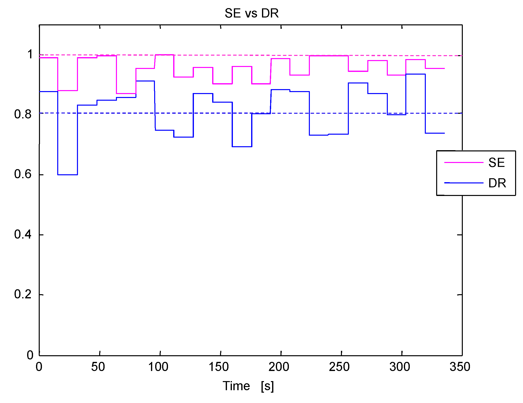
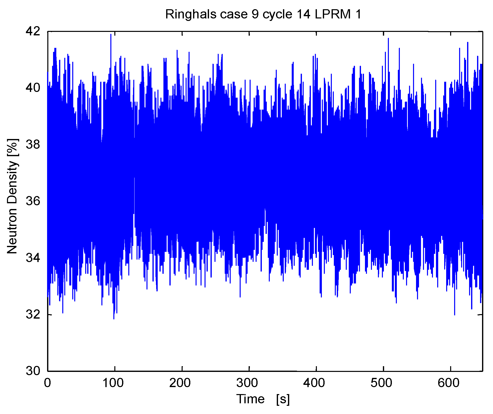
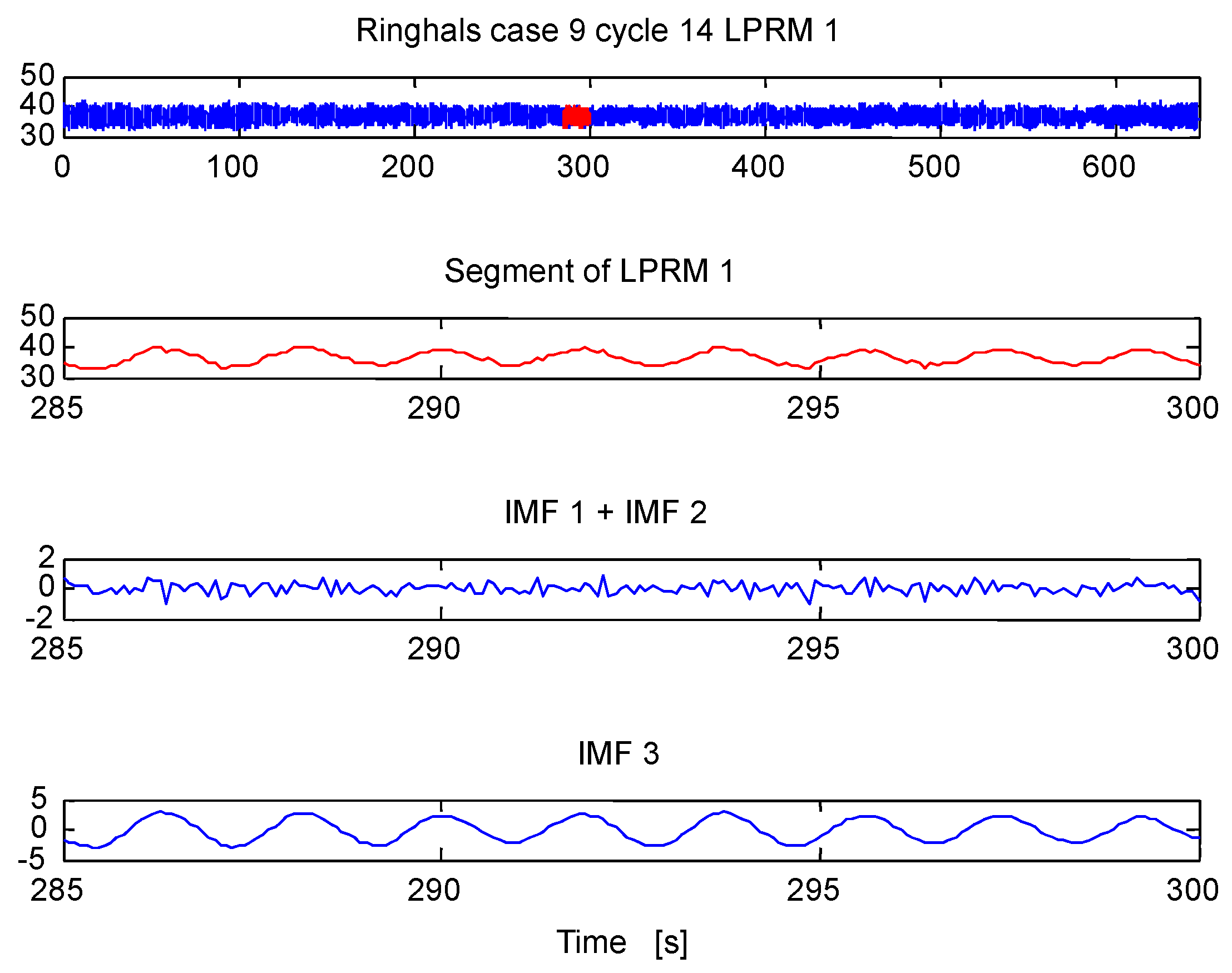
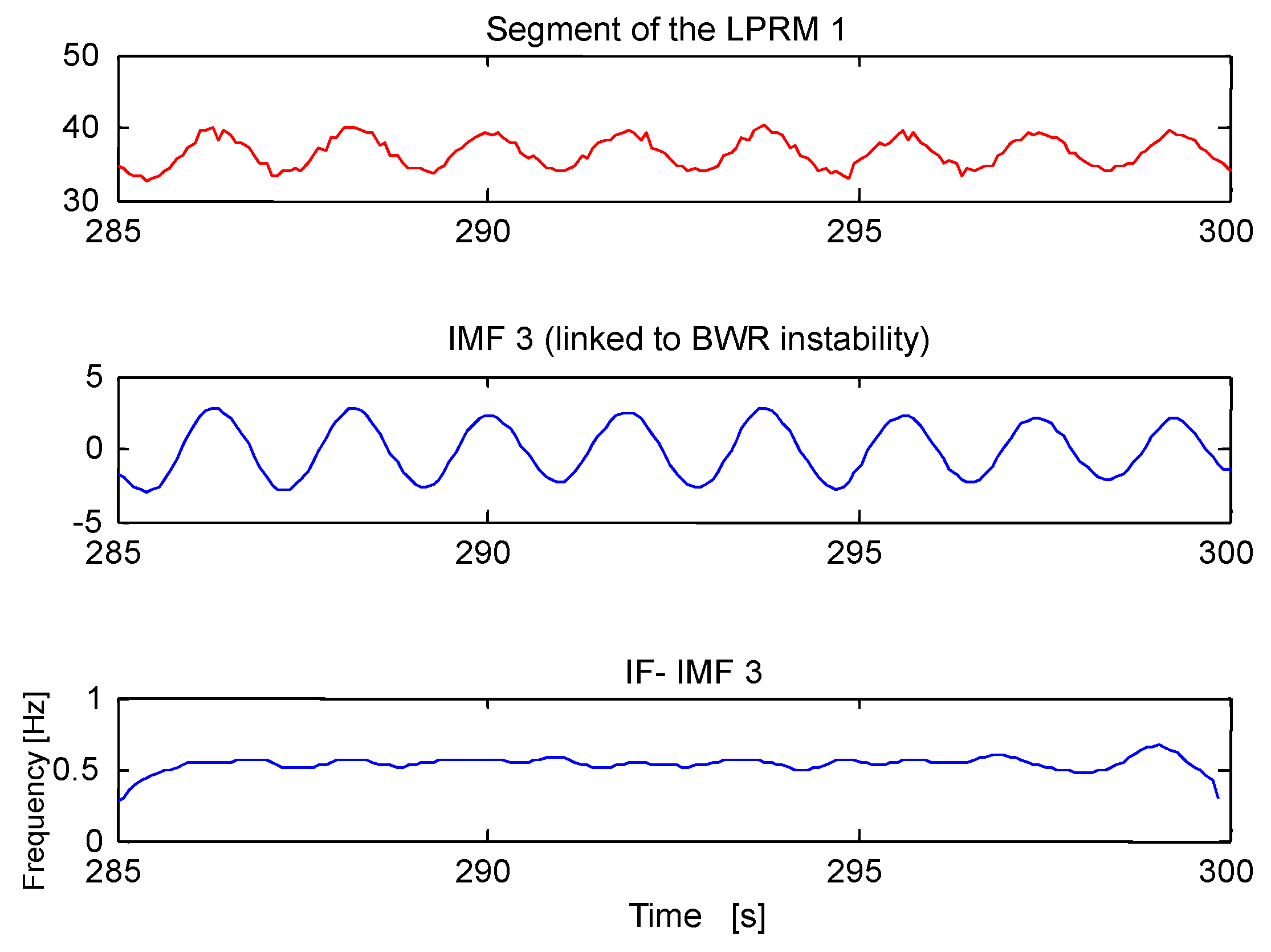
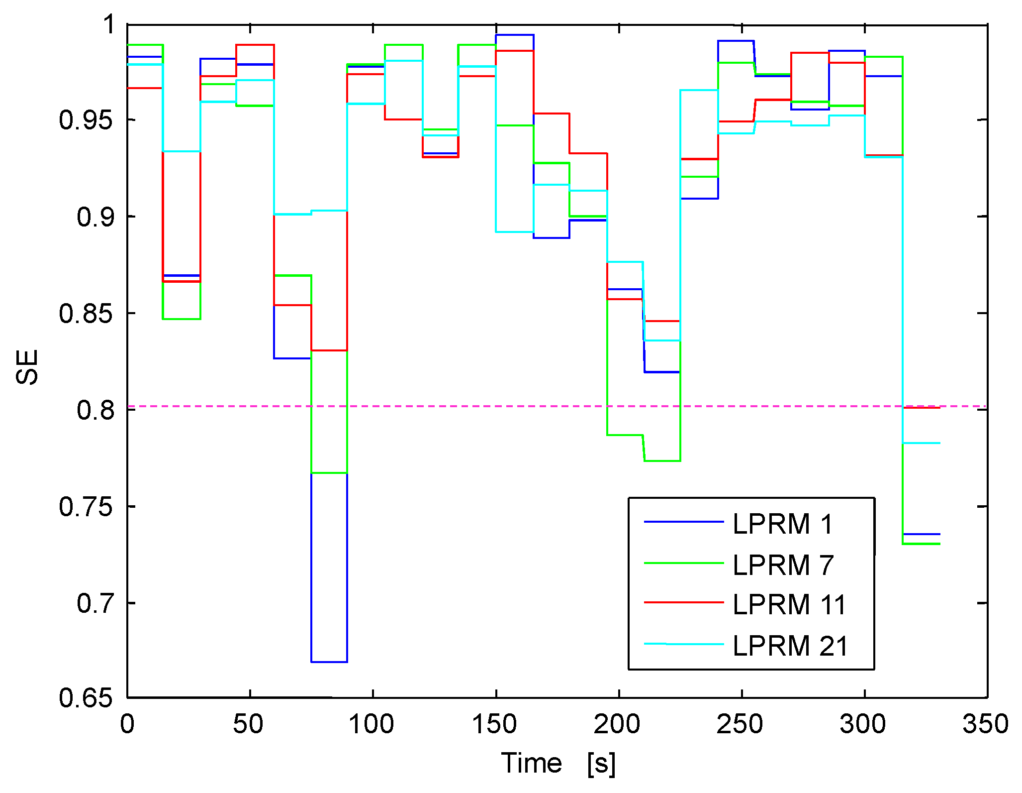
- Case 9 cycle 14 of the Ringhals stability benchmark. Data given comes from measurements in the Swedish BWR reactor Ringhals 1. This case consists of a total of 36 LPRMs. Again, the whole Case 9 (36 LPRMs) was studied, however only the analysis of one signal (LRPM 1) is detailed in this work and the others results of LPRMs are summarized in a table.
- (III)
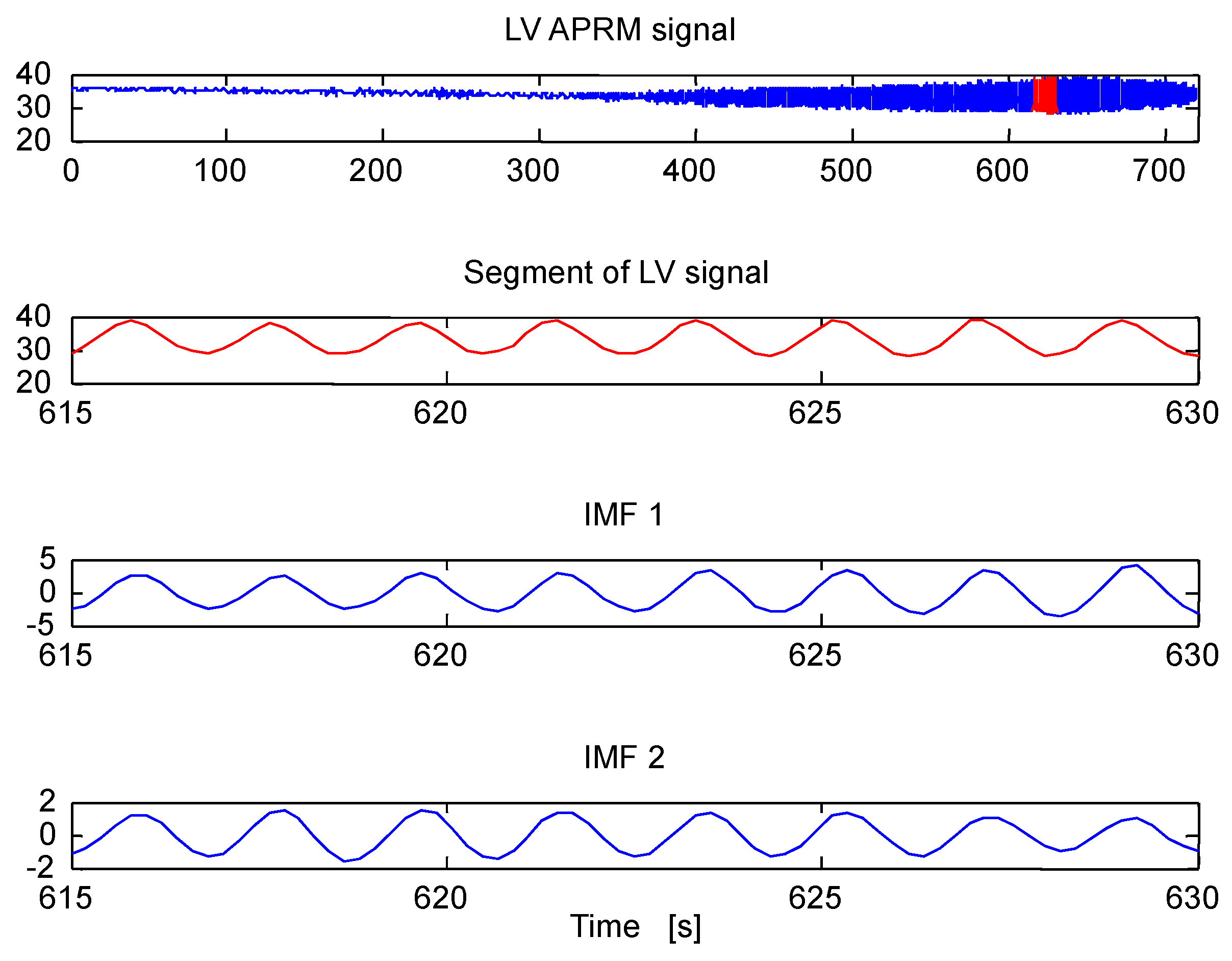
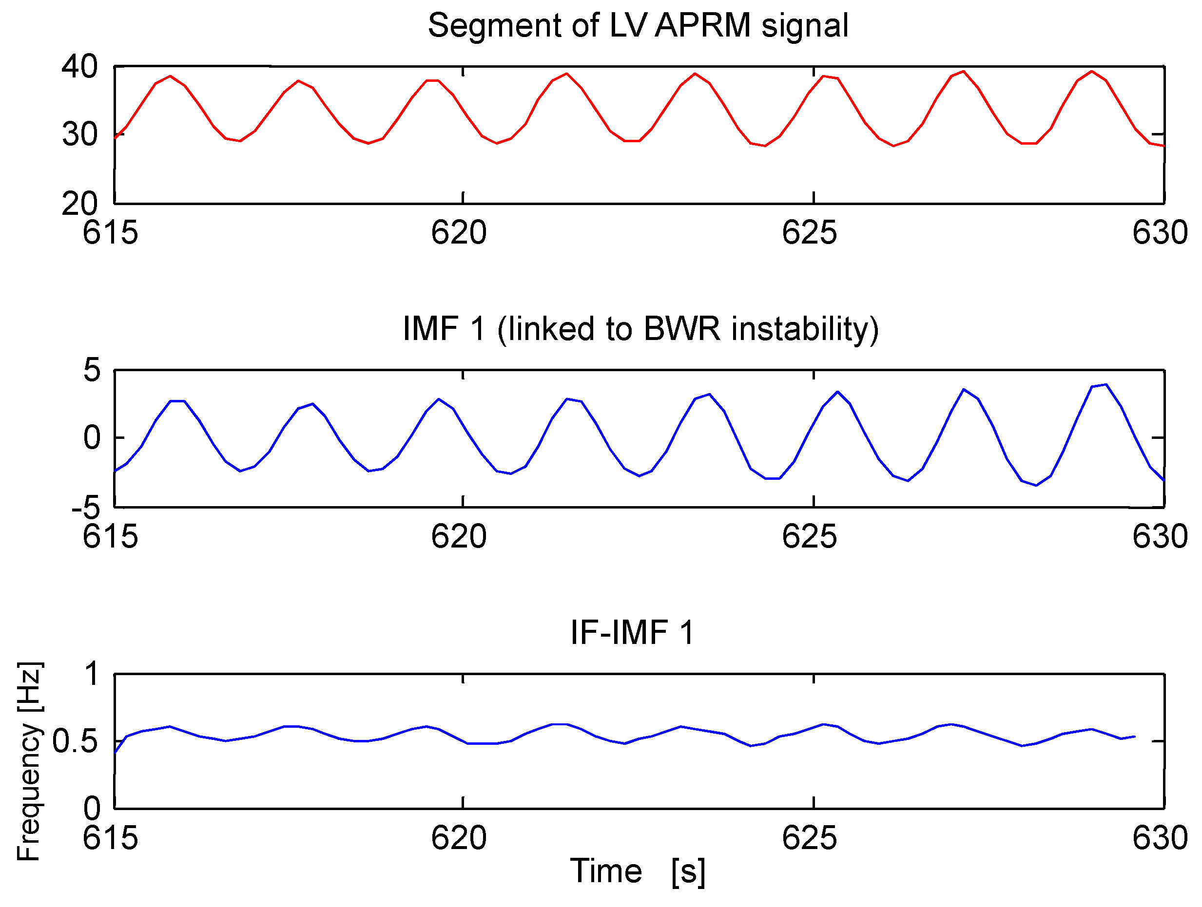
- An APRM signal that stems from the Laguna Verde BWR that was recorded during an unstable event that occurred in 1995. On 24 January 1995 a power instability event occurred in Laguna Verde Unit 1, which is a BWR-5 and is operated since 1990 at a rated power of 1931 MWt. The instability event happened during a Cycle 4 power ascension without fuel damage. When the thermal power reached 37% of the rated power, the recirculation pumps were running at low speed driving 37.8% of the total core flow. The flow control valves were set to their minimum, closed position in order to operate the recirculation pumps at a high speed. The drop in drive flow resulted in a core flow reduction of 32% and, a power reduction also of 32%. Two control rods were also partially withdrawn during valve closure. The new low flow operating conditions resulted in growing power oscillations. This prototype of in-phase instability has been widely studied [1,2,34,35,36,37].
6.1.1. APRM Signal from the Forsmark Benchmark
6.1.2. LPRM Signal from Ringhals Benchmark
6.1.3. APRM Laguna Verde
6.2. Stability Analysis of the Chosen Real Cases Through the Methodology 2
- (I)
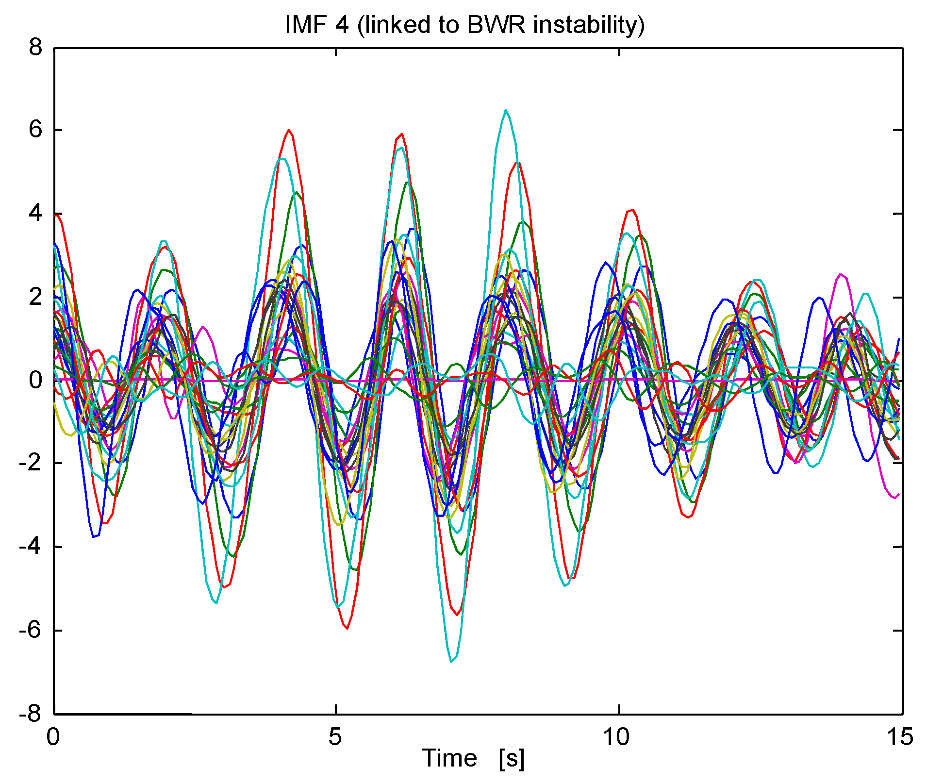
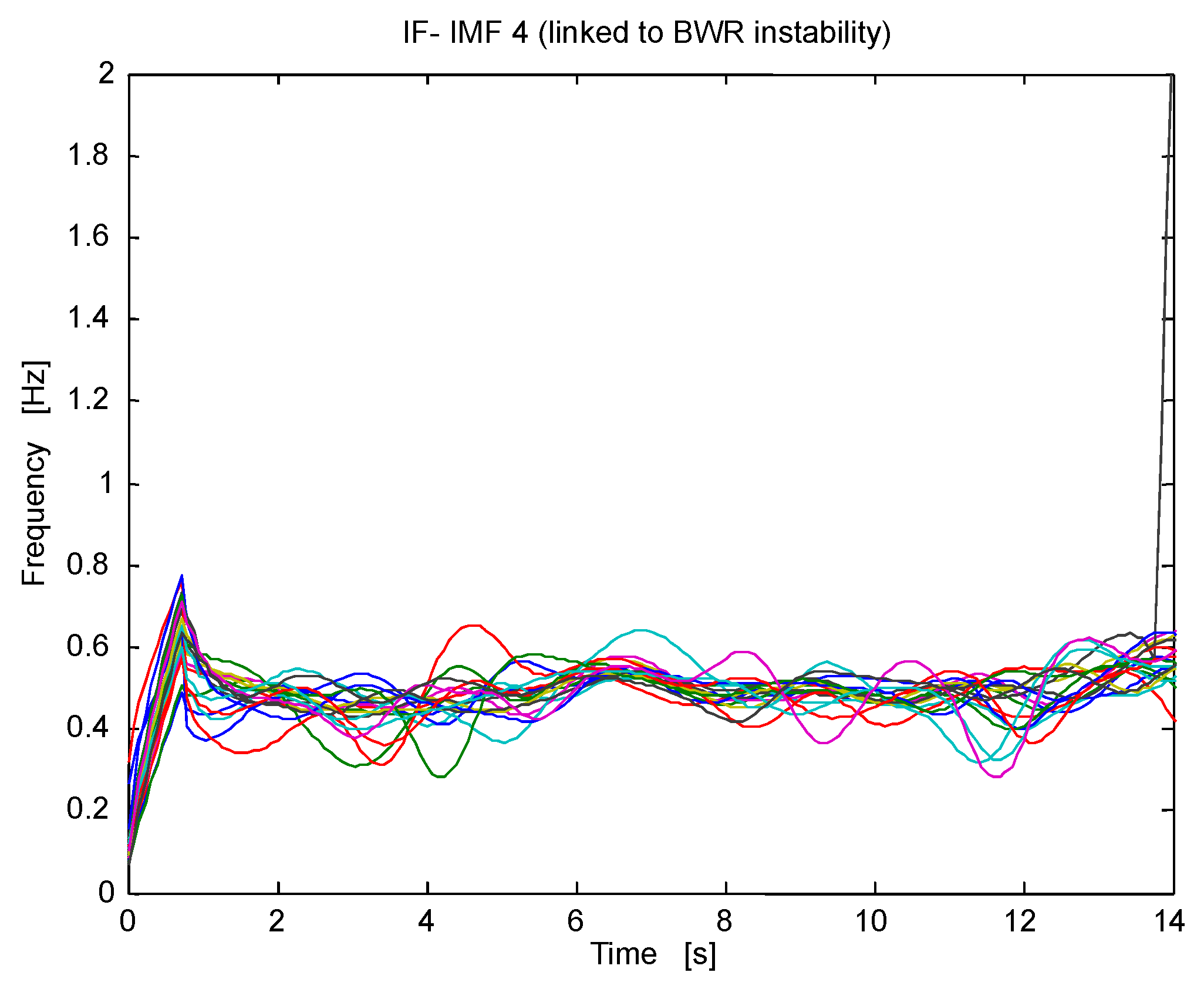
- Multidimensional analysis of the already mentioned Case 4 of the Forsmark stability benchmark.
- (II)
- Multidimensional analysis of the also mentioned Case 9 Cycle 14 of the Ringhals stability benchmark.
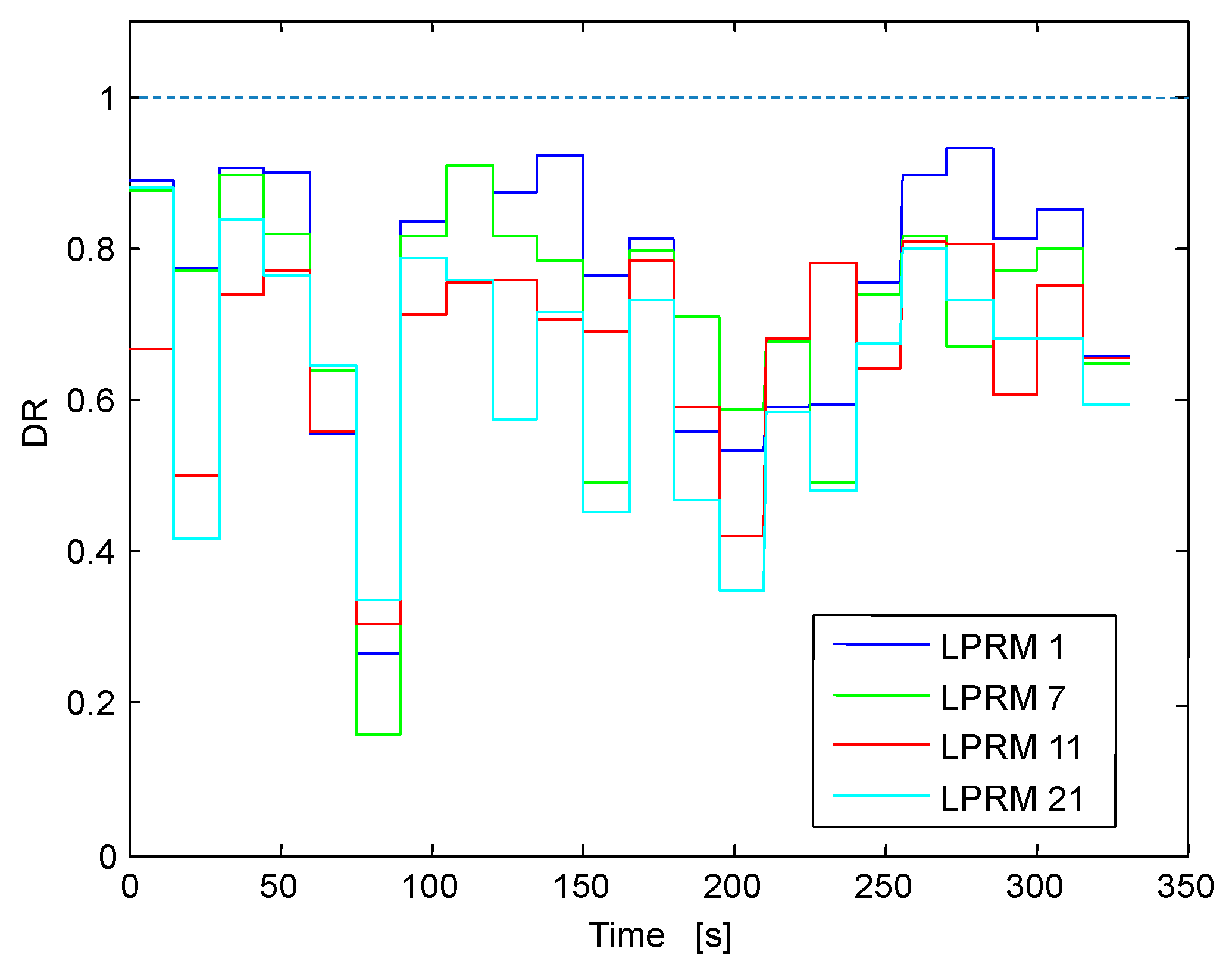
6.2.1. LPRMs Signals from Forsmark Benchmark
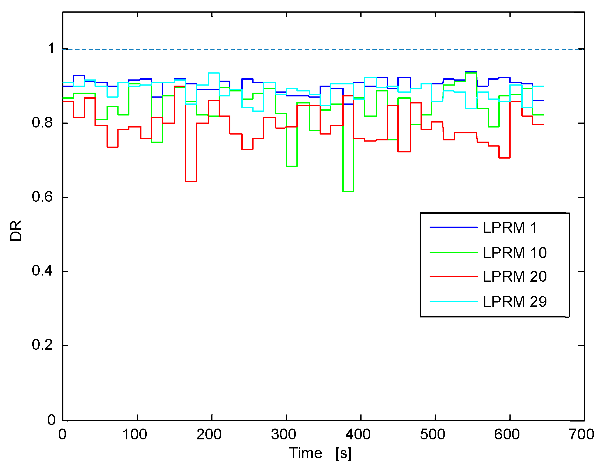
6.2.2. LPRMs from Ringhals Benchmark
6.3. Discussion and Remarks
7. Conclusions
Acknowledgments
Author Contributions
Conflicts of Interest
References
- Gonzalez, V.M.; Amador, R.; Castillo, R. Análisis del Evento de Oscilaciones de Potencia en la CNLV: Informe Preliminar; CNSNS-TR-13, REVISION 0; Comisión Nacional de Seguridad Nuclear y Salvaguardias: Mexico City, Mexico, 1995. [Google Scholar]
- Farawila, Y.M.; Pruitt, D.W.; Smith, P.E.; Sanchez, L.; Fuentes, L.P. Analysis of the Laguna Verde instability event. In Proceedings of the National Heat Transfer Conference, Houston, TX, USA, 3–6 August 1996; Volume 9, pp. 198–202. [Google Scholar]
- Verdú, G.; Ginestar, D.; Muñoz-Cobo, J.L.; Navarro-Esbrí, J.; Palomo, M.J.; Lansaker, P.; Conde, J.M.; Recio, M.; Sartori, E. Forsmark 1&2 Stability Benchmark. Time Series Analysis Methods for Oscillations during BWR Operation; Final Report, NEA/NSC/DOC(2001)2; Nuclear Science: New York, NY, USA, 2001. [Google Scholar]
- Lahey, R.T.; Podoswski, M.Z. On the analysis of various instabilities in two-phase flow. Multiph. Sci. Technol. 1989, 4, 183–371. [Google Scholar] [CrossRef]
- Van der Hagen, T.H.; Zboray, R.; de Kruijf, W.J. Questioning the use of the decay ratio in BWR stability monitoring. Ann. Nucl. Energy 2000, 27, 727–732. [Google Scholar] [CrossRef]
- Pazsit, I. Determination of reactor stability in case of dual oscillations. Ann. Nucl. Energy 1995, 22, 377–387. [Google Scholar] [CrossRef]
- Gialdi, E.; Grifoni, S.; Parmeggiani, C.; Tricoli, C. Core stability in operating BWR: Operational experience. Prog. Nucl. Energy 1985, 15, 447–459. [Google Scholar] [CrossRef]
- Navarro-Esbri, J.; Ginestar, D.; Verdu, G. Time dependence of linear stability parameters of a BWR. Prog. Nucl. Energy 2003, 43, 187–194. [Google Scholar] [CrossRef]
- Espinosa-Paredes, G.; Prieto-Guerrero, A.; Nuñez-Carrera, A.; Amador-Garcia, R. Wavelet-based method for instability analysis in boiling water reactors. Nucl. Technol. 2005, 151, 250–260. [Google Scholar]
- Espinosa-Paredes, G.; Núñez-Carrera, A.; Prieto-Guerrero, A.; Ceceñas, M. Wavelet approach for analysis of neutronic power using data of ringhals stability benchmark. Nucl. Eng. Des. 2007, 237, 1009–1015. [Google Scholar] [CrossRef]
- Sunde, C.; Pazsit, I. Wavelet techniques for the determination of the decay ratio in boiling water reactors. Kerntechnik 2007, 72, 7–19. [Google Scholar] [CrossRef]
- Castillo, R.; Alonso, G.; Palacios, J.C. Determination of limit cycles using both the slope of correlation integral and dominant Lyapunov methods. Nucl. Technol. 2004, 145, 139–149. [Google Scholar]
- Gavilán-Moreno, C.J.; Espinosa-Paredes, G. Using Largest Lyapunov Exponent to Confirm the Intrinsic Stability of Boiling Water Reactors. Nucl. Eng. Technol. 2016, 48, 434–447. [Google Scholar] [CrossRef]
- Shannon, C.E. A mathematical theory of communication. Bell Syst. Tech. J. 1948, 27, 379–423. [Google Scholar] [CrossRef]
- Colominas, M.A.; Schlotthauer, G.; Torres, M.E. Improved complete ensemble emd: A suitable tool for biomedical signal processing. Biomed. Signal Process. Control 2014, 14, 19–29. [Google Scholar] [CrossRef]
- Ur Rehman, N.; Mandic, D.P. Filter bank property of multivariate empirical mode decomposition. IEEE Trans. Signal Process. 2011, 59, 2421–2426. [Google Scholar] [CrossRef]
- Huang, N.E.; Shen, Z.; Long, S.R.; Wu, M.C.; Shih, H.H.; Zheng, Q.; Yen, N.C.; Tung, C.C.; Liu, H.H. The Empirical Mode Decomposition and the Hilbert Spectrum for Nonlinear and Non-Stationary Time Series Analysis; The Royal Society: London, UK, 1998; pp. 903–995. [Google Scholar]
- Olvera-Guerrero, O.A.; Prieto-Guerrero, A.; Espinosa-Paredes, G. Non-linear Boiling Water Reactor Stability with Shannon Entropy. Ann. Nucl. Energy 2017, 108, 1–9. [Google Scholar] [CrossRef]
- Sharma, R.; Pachori, R.B.; Acharya, U.R. Application of entropy measures on intrinsic mode functions for the automated identification of focal electroencephalogram signals. Entropy 2015, 17, 669–691. [Google Scholar] [CrossRef]
- Huang, J.R.; Fan, S.Z.; Abbod, M.F.; Jen, K.K.; Wu, J.F.; Shieh, J.S. Application of multivariate empirical mode decomposition and sample entropy in EEG signals via artificial neural networks for interpreting depth of anesthesia. Entropy 2013, 15, 3325–3339. [Google Scholar] [CrossRef]
- Zhan, L.; Li, C. A comparative study of empirical mode decomposition-based filtering for impact signal. Entropy 2016, 19, 13. [Google Scholar] [CrossRef]
- Hu, M.; Liang, H. Intrinsic mode entropy based on multivariate empirical mode decomposition and its application to neural data analysis. Cogn. Neurodyn. 2011, 5, 277–284. [Google Scholar] [CrossRef] [PubMed]
- Tseng, C.Y.; Lee, H.C. Entropic interpretation of empirical mode decomposition and its applications in signal processing. Adv. Adapt. Data Anal. 2010, 2, 429–449. [Google Scholar] [CrossRef]
- Prieto-Guerrero, A.; Espinosa-Paredes, G. Decay ratio estimation in boiling water reactors based on the empirical mode decomposition and the Hilbert–Huang transform. Prog. Nucl. Energy 2014, 71, 122–133. [Google Scholar] [CrossRef]
- Olvera-Guerrero, O.A.; Prieto-Guerrero, A.; Espinosa-Paredes, G. Decay Ratio estimation in BWRs based on the improved complete ensemble empirical mode decomposition with adaptive noise. Ann. Nucl. Energy 2017, 102, 280–296. [Google Scholar] [CrossRef]
- BWR/6. BWR/6 General Description of a Boiling Water Reactor, Nuclear Energy Division, General Electric Company; GE Nuclear Energy: Wilmington, NC, USA, 1975. [Google Scholar]
- Wu, Z.; Huang, N.E. Ensemble empirical mode decomposition: A noise assisted data analysis method. Adv. Adapt. Data Anal. 2009, 1, 1–41. [Google Scholar] [CrossRef]
- Torres, M.E.; Colominas, M.A.; Schlotthauer, G.; Flandrin, P. A complete ensemble empirical mode decomposition with adaptive noise. In Proceedings of the IEEE International Conference on Acoustics, Speech and Signal Processing (ICASSP), Prague, Czech Republic, 22–27 May 2011; pp. 4144–4147. [Google Scholar]
- Colominas, M.A.; Schlotthauer, G.; Torres, M.E.; Flandrin, P. Noise-assisted EMD methods in action. Adv. Adapt. Data Anal. 2012, 4, 1250025. [Google Scholar] [CrossRef]
- Rehman, N.; Mandic, D.P. Multivariate Empirical Mode Decomposition. Proc. R. Soc. A 2010, 466, 1291–1302. [Google Scholar] [CrossRef]
- Niederreiter, H. Random Number Generation and Quasi-Monte Carlo Methods; Society for Industrial and Applied Mathematics: Philadelphia, PA, USA, 1992. [Google Scholar]
- Knuth, K.H. Optimal data-based binning for histograms. arXiv, 2006; arXiv:physics/0605197v1. [Google Scholar]
- Lefvert, T. OECD/NEA Ringhals 1 Stability Benchmark; Nuclear Energy Agency: Boulogne-Billancourt, France, 1996. [Google Scholar]
- Blazquez, J.; Ruiz, J. The Laguna Verde BWR/5 instability Event. Prog. Nucl. Energy 2003, 43, 195–200. [Google Scholar] [CrossRef]
- Nuñez-Carrera, A.; Espinosa-Paredes, G. Time-Scale BWR stability analysis using wavelet-based method. Prog. Nucl. Energy 2006, 48, 540–549. [Google Scholar] [CrossRef]
- Prieto-Guerrero, A.; Espinosa-Paredes, G. Decay Ratio Estimation of BWR Signals based on Wavelet Ridges. Nucl. Sci. Eng. 2008, 160, 302–317. [Google Scholar] [CrossRef]
- Moreno, C.G. Boiling water reactor instability analysis using attractor characteristics. Ann. Nucl. Energy 2016, 88, 41–48. [Google Scholar] [CrossRef]
- Prieto-Guerrero, A.; Espinosa-Paredes, G.; Laguna-Sánchez, G.A. Stability monitor for boiling water reactors based on the multivariate empirical mode decomposition. Ann. Nucl. Energy 2015, 85, 453–460. [Google Scholar] [CrossRef]
- March-Leuba, J.; Blakeman, E.D. A mechanism for out-of-phase power instabilities in Boiling Water Reactors. Nucl. Sci. Eng. 1991, 107, 173–179. [Google Scholar]
- Muñoz-Cobo, J.L.; Escrivá, A.; Domingo, M.D. In-phase instabilities in BWR with sub-cooled boiling, direct heating, and spacers effects. Ann. Nucl. Energy 2016, 87, 671–686. [Google Scholar] [CrossRef]
- Dokhane, A.; Hennig, D.; Chawla, R. Interpretation of in-phase and out-of-phase BWR oscillations using an extended reduced order model and semi-analytical bifurcation analysis. Ann. Nucl. Energy 2007, 34, 271–287. [Google Scholar] [CrossRef]
- Demeshko, M.; Dokhane, A.; Washio, T.; Ferroukhi, H.; Kawahara, Y.; Aguirre, C. Application of Continuous and Structural ARMA modeling for noise analysis of a BWR coupled core and plant instability event. Ann. Nucl. Energy 2015, 75, 645–657. [Google Scholar] [CrossRef]
- Paul, S.; Singh, S. A density variant drift flux model for density wave oscillations. Int. J. Heat Mass Transf. 2014, 69, 151–163. [Google Scholar] [CrossRef]
- Paul, S.; Singh, S. On nonlinear dynamics of density wave oscillations in a channel with non-uniform axial heating. Int. J. Therm. Sci. 2017, 116, 172–198. [Google Scholar] [CrossRef]
- Vinai, P.; Demazière, C.; Dykin, V. Modelling of a self-sustained density wave oscillation and its neutronic response in a three-dimensional heterogeneous system. Ann. Nucl. Energy 2014, 67, 41–48. [Google Scholar] [CrossRef]
- Paruya, S.; Goswami, N.; Pushpavanam, S.; Pillai, D.S.; Bidyarani, O. Periodically-forced density wave oscillations in boiling flow at low forcing frequencies: Nonlinear dynamics and control issues. Chem. Eng. Sci. 2016, 140, 123–133. [Google Scholar] [CrossRef]
- Pandey, V.; Singh, S. Characterization of stability limits of Ledinegg instability and density wave oscillations for two-phase flow in natural circulation loops. Chem. Eng. Sci. 2017, 168, 204–224. [Google Scholar] [CrossRef]
- Marcel, C.P.; Rohde, M.; Van Der Hagen, T.H.J.J. An experimental parametric study on natural circulation BWRs stability. Nucl. Eng. Des. 2017, 318, 135–146. [Google Scholar] [CrossRef]
- Castillo-Durán, R.; Ortiz-Servin, J.J.; Castillo, A.; Montes-Tadeo, J.L.; Perusquía-del-Cueto, R. A stability assessment of optimum Fuel Reload Patterns for a BWR. Ann. Nucl. Energy 2016, 94, 841–847. [Google Scholar] [CrossRef]


| Detectors | Mean SE | Std SE | Mean DR | Std DR | Mean f0 | Std f0 |
|---|---|---|---|---|---|---|
| APRM | 0.9553 | 0.0377 | 0.8136 | 0.0842 | 0.5279 | 0.0299 |
| LPRM 1 | 0.9527 | 0.0236 | 0.801 | 0.0765 | 0.519 | 0.0282 |
| LPRM 2 | 0.9564 | 0.0344 | 0.8007 | 0.1048 | 0.5101 | 0.03 |
| LPMR 3 | 0.9607 | 0.0222 | 0.8211 | 0.0778 | 0.5036 | 0.0202 |
| LPMR 4 | 0.9515 | 0.0268 | 0.7649 | 0.123 | 0.5116 | 0.0345 |
| LPRM 5 | 0.9323 | 0.0493 | 0.771 | 0.1269 | 0.5424 | 0.0317 |
| LPRM 6 | 0.9422 | 0.0304 | 0.765 | 0.1376 | 0.5444 | 0.0265 |
| LPRM 7 | 0.9409 | 0.0313 | 0.7623 | 0.0843 | 0.5513 | 0.0346 |
| LPMR 8 | 0.921 | 0.0411 | 0.6991 | 0.0873 | 0.5683 | 0.0509 |
| LPRM 9 | 0.9331 | 0.049 | 0.752 | 0.0966 | 0.5461 | 0.0384 |
| LPRM 10 | 0.9272 | 0.0429 | 0.7043 | 0.1315 | 0.574 | 0.0373 |
| LPRM 11 | 0.9224 | 0.0586 | 0.7527 | 0.0885 | 0.5513 | 0.0425 |
| LPRM 12 | 0.9074 | 0.0521 | 0.545 | 0.1649 | 0.5796 | 0.078 |
| LPRM 13 | 0.9436 | 0.0356 | 0.7753 | 0.1208 | 0.5462 | 0.0315 |
| LPRM 14 | 0.9334 | 0.0396 | 0.7783 | 0.0907 | 0.5386 | 0.0397 |
| LPRM 15 | 0.9428 | 0.0356 | 0.7569 | 0.1241 | 0.537 | 0.0408 |
| LPMR 16 | 0.9477 | 0.0331 | 0.7831 | 0.092 | 0.5362 | 0.0341 |
| LPMR 17 | 0.9449 | 0.0375 | 0.7683 | 0.089 | 0.5302 | 0.0486 |
| LPRM 18 | 0.9489 | 0.0375 | 0.7487 | 0.1392 | 0.5253 | 0.0362 |
| LPRM 19 | 0.915 | 0.0575 | 0.6295 | 0.1206 | 0.5111 | 0.0703 |
| LPRM 20 | 0.9152 | 0.0429 | 0.6834 | 0.1149 | 0.5631 | 0.0487 |
| LPMR 21 | 0.9227 | 0.0368 | 0.6841 | 0.1882 | 0.5777 | 0.0566 |
| LPRM 22 | 0.9026 | 0.0408 | 0.518 | 0.1275 | 0.5606 | 0.1011 |
| Detectors | Mean SE | Std SE | Mean DR | Std DR | Mean f0 | Std f0 |
|---|---|---|---|---|---|---|
| LPRM 1 | 0.9809 | 0.0084 | 0.9132 | 0.0161 | 0.5164 | 0.0248 |
| LPRM 3 | 0.9826 | 0.0069 | 0.9122 | 0.0171 | 0.5153 | 0.0226 |
| LPRM 5 | 0.9834 | 0.0094 | 0.9102 | 0.0162 | 0.5157 | 0.0246 |
| LPRM 7 | 0.9877 | 0.0153 | 0.8897 | 0.0367 | 0.5149 | 0.0243 |
| LPRM 9 | 0.9854 | 0.0082 | 0.9135 | 0.0184 | 0.5139 | 0.0266 |
| LPRM 11 | 0.9823 | 0.0078 | 0.9134 | 0.0172 | 0.5175 | 0.0248 |
| LPRM 13 | 0.9820 | 0.0106 | 0.9108 | 0.0214 | 0.5169 | 0.0219 |
| LPRM 15 | 0.9856 | 0.0088 | 0.9091 | 0.0179 | 0.5106 | 0.0270 |
| LPRM 17 | 0.9883 | 0.0080 | 0.9006 | 0.0221 | 0.5188 | 0.0241 |
| LPRM 19 | 0.9621 | 0.0436 | 0.8332 | 0.0778 | 0.5180 | 0.0274 |
| LPRM 21 | 0.9814 | 0.0270 | 0.8693 | 0.0506 | 0.5218 | 0.0267 |
| LPRM 23 | 0.9862 | 0.0149 | 0.8909 | 0.0301 | 0.5174 | 0.0248 |
| LPRM 25 | 0.9841 | 0.0122 | 0.8997 | 0.0273 | 0.5125 | 0.0267 |
| LPRM 27 | 0.9869 | 0.0142 | 0.8951 | 0.0352 | 0.5136 | 0.0281 |
| LPRM 29 | 0.9653 | 0.0509 | 0.8309 | 0.0762 | 0.5186 | 0.0364 |
| LPRM 31 | 0.9500 | 0.0441 | 0.8106 | 0.0820 | 0.5049 | 0.0348 |
| LPRM 33 | 0.9429 | 0.0409 | 0.6562 | 0.1321 | 0.4868 | 0.0286 |
| LPRM 35 | 0.9630 | 0.0352 | 0.7145 | 0.2115 | 0.5020 | 0.0365 |
| LPRM 37 | 0.9771 | 0.0203 | 0.8538 | 0.0490 | 0.5124 | 0.0272 |
| LPRM 39 | 0.9598 | 0.0335 | 0.7558 | 0.0766 | 0.5062 | 0.0338 |
| LPRM 41 | 0.9141 | 0.0637 | 0.5868 | 0.2425 | 0.4987 | 0.0423 |
| LPRM 43 | 0.8814 | 0.0672 | 0.4893 | 0.2241 | 0.4922 | 0.0386 |
| LPRM 45 | 0.9858 | 0.0124 | 0.8496 | 0.0415 | 0.5126 | 0.0265 |
| LPRM 47 | 0.9854 | 0.0094 | 0.8816 | 0.0284 | 0.5071 | 0.0242 |
| LPRM 49 | 0.9807 | 0.0091 | 0.9110 | 0.0173 | 0.5102 | 0.0279 |
| LPRM 51 | 0.9771 | 0.0086 | 0.9120 | 0.0133 | 0.5121 | 0.0218 |
| LPRM 53 | 0.9823 | 0.0077 | 0.9096 | 0.0184 | 0.5154 | 0.0262 |
| LPRM 55 | 0.9868 | 0.0091 | 0.8974 | 0.0250 | 0.5204 | 0.0218 |
| LPRM 57 | 0.9804 | 0.0076 | 0.9061 | 0.0143 | 0.5195 | 0.0188 |
| LPRM 59 | 0.9771 | 0.0087 | 0.9084 | 0.0149 | 0.5126 | 0.0223 |
| LPRM 61 | 0.9765 | 0.0101 | 0.9126 | 0.0149 | 0.5140 | 0.0229 |
| LPRM 63 | 0.9764 | 0.0089 | 0.9123 | 0.0137 | 0.5112 | 0.0245 |
| LPRM 65 | 0.9805 | 0.0085 | 0.9059 | 0.0185 | 0.5117 | 0.0268 |
| LPRM 67 | 0.9832 | 0.0113 | 0.9054 | 0.0202 | 0.5149 | 0.0223 |
| LPRM 69 | 0.9817 | 0.0093 | 0.9023 | 0.0184 | 0.5155 | 0.0197 |
| LPRM 71 | 0.9831 | 0.0073 | 0.9029 | 0.0181 | 0.5156 | 0.0253 |
| Detector | Mean SE | Std SE | Mean DR | Std DR | Mean f0 | Std f0 |
|---|---|---|---|---|---|---|
| APRM | 0.9592 | 0.0444 | 1.0079 | 0.1655 | 0.5385 | 0.0158 |
| Detectors | Mean SE | Std SE | Mean DR | Std DR | Mean f0 | Std f0 |
|---|---|---|---|---|---|---|
| LPRM 1 | 0.9208 | 0.0816 | 0.7669 | 0.1417 | 0.4754 | 0.0283 |
| LPRM 2 | 0.9220 | 0.0842 | 0.7670 | 0.1526 | 0.4867 | 0.0250 |
| LPMR 3 | 0.9164 | 0.0924 | 0.7791 | 0.1457 | 0.4875 | 0.0260 |
| LPMR 4 | 0.9034 | 0.1001 | 0.7551 | 0.1476 | 0.4867 | 0.0214 |
| LPRM 5 | 0.9278 | 0.0762 | 0.7328 | 0.1585 | 0.5030 | 0.0373 |
| LPRM 6 | 0.9234 | 0.0783 | 0.7383 | 0.1338 | 0.5034 | 0.0357 |
| LPRM 7 | 0.9176 | 0.0789 | 0.7232 | 0.1232 | 0.5012 | 0.0368 |
| LPMR 8 | 0.9160 | 0.0761 | 0.6595 | 0.1511 | 0.5047 | 0.0447 |
| LPRM 9 | 0.9241 | 0.0767 | 0.6749 | 0.1703 | 0.5016 | 0.0355 |
| LPRM 10 | 0.9127 | 0.0700 | 0.6131 | 0.1748 | 0.5129 | 0.0425 |
| LPRM 11 | 0.9278 | 0.0618 | 0.6466 | 0.1482 | 0.4980 | 0.0395 |
| LPRM 12 | 0.9167 | 0.0450 | 0.5177 | 0.1378 | 0.5163 | 0.0636 |
| LPRM 13 | 0.9218 | 0.0721 | 0.7076 | 0.1327 | 0.5020 | 0.0292 |
| LPRM 14 | 0.9130 | 0.0756 | 0.6945 | 0.1537 | 0.5047 | 0.0300 |
| LPRM 15 | 0.9162 | 0.0785 | 0.7021 | 0.1281 | 0.5028 | 0.0385 |
| LPMR 16 | 0.9108 | 0.0889 | 0.7145 | 0.1088 | 0.5018 | 0.0299 |
| LPMR 17 | 0.9235 | 0.0814 | 0.7331 | 0.1506 | 0.4927 | 0.0242 |
| LPRM 18 | 0.9233 | 0.0851 | 0.7158 | 0.1693 | 0.4990 | 0.0282 |
| LPRM 19 | 0.9235 | 0.0670 | 0.6521 | 0.1686 | 0.4947 | 0.0477 |
| LPRM 20 | 0.9060 | 0.0884 | 0.6337 | 0.1861 | 0.5020 | 0.0428 |
| LPMR 21 | 0.9256 | 0.0668 | 0.6290 | 0.1512 | 0.5037 | 0.0413 |
| LPRM 22 | 0.8900 | 0.0593 | 0.4413 | 0.1466 | 0.5118 | 0.0840 |
| Detectors | Mean SE | Std SE | Mean DR | Std DR | Mean f0 | Std f0 |
|---|---|---|---|---|---|---|
| LPRM 1 | 0.9792 | 0.0064 | 0.9033 | 0.0170 | 0.5271 | 0.0223 |
| LPRM 3 | 0.9779 | 0.0062 | 0.9006 | 0.0158 | 0.5284 | 0.0215 |
| LPRM 5 | 0.9786 | 0.0089 | 0.8997 | 0.0194 | 0.5286 | 0.0209 |
| LPRM 7 | 0.9793 | 0.0091 | 0.8841 | 0.0315 | 0.5251 | 0.0235 |
| LPRM 9 | 0.9791 | 0.0057 | 0.9003 | 0.0207 | 0.5244 | 0.0268 |
| LPRM 11 | 0.9792 | 0.0065 | 0.9007 | 0.0206 | 0.5270 | 0.0237 |
| LPRM 13 | 0.9762 | 0.0087 | 0.9005 | 0.0196 | 0.5306 | 0.0182 |
| LPRM 15 | 0.9790 | 0.0070 | 0.8977 | 0.0196 | 0.5256 | 0.0247 |
| LPRM 17 | 0.9808 | 0.0083 | 0.8910 | 0.0237 | 0.5239 | 0.0260 |
| LPRM 19 | 0.9708 | 0.0192 | 0.8468 | 0.0594 | 0.5373 | 0.0073 |
| LPRM 21 | 0.9750 | 0.0121 | 0.8682 | 0.0421 | 0.5337 | 0.0141 |
| LPRM 23 | 0.9802 | 0.0086 | 0.8894 | 0.0266 | 0.5307 | 0.0193 |
| LPRM 25 | 0.9789 | 0.0074 | 0.8930 | 0.0230 | 0.5286 | 0.0221 |
| LPRM 27 | 0.9776 | 0.0141 | 0.8881 | 0.0360 | 0.5314 | 0.0189 |
| LPRM 29 | 0.9728 | 0.0229 | 0.8402 | 0.0591 | 0.5346 | 0.0181 |
| LPRM 31 | 0.9635 | 0.0363 | 0.8150 | 0.0792 | 0.5381 | 0.0140 |
| LPRM 33 | 0.9648 | 0.0187 | 0.7227 | 0.1068 | 0.5318 | 0.0224 |
| LPRM 35 | 0.9681 | 0.0213 | 0.7680 | 0.0865 | 0.5308 | 0.0196 |
| LPRM 37 | 0.9769 | 0.0123 | 0.8573 | 0.0393 | 0.5304 | 0.0166 |
| LPRM 39 | 0.9731 | 0.0113 | 0.7923 | 0.0483 | 0.5310 | 0.0228 |
| LPRM 41 | 0.9544 | 0.0306 | 0.6935 | 0.1651 | 0.5312 | 0.0324 |
| LPRM 43 | 0.9600 | 0.0295 | 0.7080 | 0.1310 | 0.5368 | 0.0316 |
| LPRM 45 | 0.9471 | 0.0349 | 0.5754 | 0.2262 | 0.5408 | 0.0456 |
| LPRM 47 | 0.9782 | 0.0073 | 0.8511 | 0.0418 | 0.5279 | 0.0199 |
| LPRM 49 | 0.9796 | 0.0074 | 0.8805 | 0.0255 | 0.5310 | 0.0162 |
| LPRM 51 | 0.9803 | 0.0065 | 0.8992 | 0.0179 | 0.5299 | 0.0169 |
| LPRM 53 | 0.9786 | 0.0055 | 0.8999 | 0.0149 | 0.5271 | 0.0194 |
| LPRM 55 | 0.9813 | 0.0043 | 0.8970 | 0.0195 | 0.5293 | 0.0185 |
| LPRM 57 | 0.9802 | 0.0068 | 0.8868 | 0.0263 | 0.5274 | 0.0204 |
| LPRM 59 | 0.9730 | 0.0329 | 0.8719 | 0.1111 | 0.5254 | 0.0202 |
| LPRM 61 | 0.9698 | 0.0446 | 0.8734 | 0.1171 | 0.5272 | 0.0189 |
| LPRM 63 | 0.9680 | 0.0529 | 0.8790 | 0.0999 | 0.5276 | 0.0187 |
| LPRM 65 | 0.9646 | 0.0669 | 0.8737 | 0.1080 | 0.5265 | 0.0186 |
| LPRM 67 | 0.9685 | 0.0489 | 0.8734 | 0.0948 | 0.5269 | 0.0189 |
| LPRM 69 | 0.9717 | 0.0416 | 0.8735 | 0.1010 | 0.5239 | 0.0228 |
| LPRM 71 | 0.9752 | 0.0218 | 0.8722 | 0.1014 | 0.5275 | 0.0177 |
© 2017 by the authors. Licensee MDPI, Basel, Switzerland. This article is an open access article distributed under the terms and conditions of the Creative Commons Attribution (CC BY) license (http://creativecommons.org/licenses/by/4.0/).
Share and Cite
Olvera-Guerrero, O.A.; Prieto-Guerrero, A.; Espinosa-Paredes, G. Non-Linear Stability Analysis of Real Signals from Nuclear Power Plants (Boiling Water Reactors) Based on Noise Assisted Empirical Mode Decomposition Variants and the Shannon Entropy. Entropy 2017, 19, 359. https://doi.org/10.3390/e19070359
Olvera-Guerrero OA, Prieto-Guerrero A, Espinosa-Paredes G. Non-Linear Stability Analysis of Real Signals from Nuclear Power Plants (Boiling Water Reactors) Based on Noise Assisted Empirical Mode Decomposition Variants and the Shannon Entropy. Entropy. 2017; 19(7):359. https://doi.org/10.3390/e19070359
Chicago/Turabian StyleOlvera-Guerrero, Omar Alejandro, Alfonso Prieto-Guerrero, and Gilberto Espinosa-Paredes. 2017. "Non-Linear Stability Analysis of Real Signals from Nuclear Power Plants (Boiling Water Reactors) Based on Noise Assisted Empirical Mode Decomposition Variants and the Shannon Entropy" Entropy 19, no. 7: 359. https://doi.org/10.3390/e19070359