1. Introduction
The development of the derivatives market has long been a topic of interest among researchers, policy makers, and financial agencies. It directly plays a vital role in a financial system and greatly contributes to various aspects of an economy as a whole.
Lien and Zhang (
2008) summarize the roles and functions of the derivatives market in emerging economies, in both theoretical and empirical studies. First, the derivatives market offers an effective mechanism that facilitates the sharing of price risks for commodities traded on the market, helping producers deal with price volatility. Also, it serves as a key role in smooth hedging and risk management by enhancing capital inflows in emerging and developing countries, but it has a negative impact on financial systems by introducing more unpredictable crisis dynamics and is a driver of contagion. Second, it is widely accepted that the derivatives market functions as a channel of risk reduction and redistribution, a means of price discovery and a price stabilizer. Various derivative instruments appear to suit the risk preference of different agents, such as hedgers or spectaculars. The derivatives market is expected to increase information flows in the market. Information about future prices is more likely to reflect future demand, thus influencing production and storage decisions and eventually reducing spot price volatility.
Atilgan et al. (
2016) offer an updated survey on the literature on derivatives in emerging countries, dividing empirical studies into groups according to the function of the derivatives market. In addition to updating the function of the derivatives market on hedging and risk management as well as price discovery in the spot market, they explore issues regarding market structure and efficiency, as well as risk and price measurement.
The crucial role played by the derivatives market in the financial system is indispensable with a vast amount of research having been conducted, both theoretically and empirically. However, a debate over its effects on economic development has arisen because of a lack of supporting evidence. To the best of our knowledge, few theoretical studies mention the impact of the development of the derivatives market on economic growth (
Haiss and Sammer 2010). Some contemporary studies illustrate a link between risk and economic growth, indirectly implying one of the main roles of the derivatives market.
Acemoglu and Zilibotti (
1997) propose a model in which undiversified agent risks affect aggregate volatility and economic growth through the relocation of funding; agents tend to invest in higher-return projects that appear to have better diversification opportunities.
Krebs (
2003) reveals that the elimination of idiosyncratic risk leads to a decline in the ratio of physical to human capital and an increase in the degree of investment returns and welfare. In summary, having advanced financial tools fosters a better distribution of resources, both human and financial, to more productive activities, thus enhancing economic growth.
Our research investigates the dynamic relationship among the development of derivatives markets, economic growth, volatility, and other macroeconomic variables, namely, trade openness and interest rates. We consider the world’s four large economies with large derivatives markets—China, India, Japan, and the U.S.—which we consider jointly as the CIJU countries. The U.S. is the biggest economy with a real gross domestic product (GDP) of about
$17 trillion. China has experienced remarkable growth in its real GDP over the past two decades, now about
$8.5 billion, making it the world’s second-largest economy. Although its real GDP currently has the slowest increase, Japan is still one of the largest economies, with real GDP of around
$6 trillion. India has increased its real GDP more than threefold over this period (approximately
$2.5 trillion). The growth in real GDP is accompanied by an increase in GDP per capita in these countries (see
Table 1).
Our study contributes to the literature by focusing on the CIJU countries, which have had mature derivatives markets examining both the short- and long-run effects of the derivatives market, the trade openness, and interest rate on economic development, as well as economic growth volatility using several time-series econometric techniques that offer an analytical approach that is appropriate for the available data, and addressing potential endogeneity problems in the regression.
The remainder of the paper is organized as follows. Following this Introduction,
Section 2 reviews the relevant literature in terms of theoretical and empirical studies.
Section 3 offers an overview of the derivatives market in the CIJU countries. Then, we employ various econometric techniques to examine the nature of stationarity and co-integration of the data in
Section 4. Next, we present the data and discuss our empirical results in
Section 5. Finally, we present concluding remarks and policy implications in
Section 6.
2. Literature Review
A great deal of effort has been expanding in investigating the important influence of the development of the derivatives market on various aspects of financial systems.
Haiss and Sammer (
2010) explore the role of derivatives in the nexus between finance and growth via three channels: volume, efficiency, and risk. First, in the volume channel, the development of derivatives markets influences the financial market and economic growth by facilitating and increasing the accumulation of capital. It enhances the allocation of resources into investment activities at higher rates of return with the help of the mobility of savings and the higher potential of investment in an enormous range of risky projects. Second, the efficiency channel is a summary of several functions, such as an efficient substitute for cash market trade, resource movement across time and space, and an information provider for risk management and price strategy. It is therefore beneficial for such agents as firms, financial institutions, and the government to have a larger combination of funding sources at lower costs. Third, the risk channel is concerned with the negative impact of derivatives market development on the financial market and economic growth. It may raise speculation about underlying assets, making the financial markets more volatile and adding more uncertainty to the economy. However, using derivatives as hedging instruments could be beneficial for firms and agents (see e.g.,
Allayannis and Ofek 2001;
Bartram et al. 2009;
Hammoudeh and McAleer 2013;
Huang et al. 2017;
Tanha and Dempsey 2017).
Sendeniz-Yuncu et al. (
2018) mention that a well-functioning derivatives market makes it possible for firms to share risks efficiently and allows them to conduct projects with higher risk and consequently to boost economic growth. At the same time, agents, such as investors, consumers, and producers, can rely on the derivatives market as an information channel that reflects equilibrium prices so that they can make the right decisions, fostering the efficiency of resource distribution and consequently resulting in economic growth.
The causal relation between the futures market and economic growth in both developed and developing countries is highlighted in
Sendeniz-Yuncu et al. (
2018)’s study based on time-series data. They find that, in 29 out of the 32 countries studied, the two variables of concern have a long-run relationship and that middle-income countries have a Granger-causality effect from the futures market to economic growth while in high-income countries the effect is reversed. These authors distinguish these opposite unidirectional causations between futures market development and economic growth. On the one hand, the direction starts with futures market development to economic growth in most countries with relatively low real GDP per capita. On the other hand, in countries with a relatively high real per capita GDP, economic growth tends to lead to the development of a futures market. Like
Khan et al. (
2017) using a panel vector autoregressive method and the Granger causality approach,
Vo et al. (
2019) show the existence of bidirectional Granger causality between the derivatives market and economic growth, although the causal relation differs between high- and middle-income countries.
The empirical studies focus on the links between economic growth and financial market development, rather than the derivatives market. Various research has approached economic growth via the development of financial intermediaries, such as banking sector development (
Beck et al. 2000;
King and Levine 1993;
Levine et al. 2000;
Levine 2005;
Menyah et al. 2014;
Pradhan et al. 2014;
Chaiechi 2012), stock market development (
Tsouma 2009;
Ang and Mckibbin 2007;
Huang et al. 2000), and bond market development (
Coskun et al. 2017;
Thumrongvit et al. 2013).
1 Pradhan et al. (
2014) conduct an analysis on paired relations among four economic components—including the banking sector, stocks, and economic growth—and macro variables, such as foreign direct investment (FDI), trade openness, inflation rate, and government consumption and expenditure. Of these selected variables, the financial sector, banking, and the derivatives market are found to boost economic growth, whereas the macro variables, namely FDI and trade openness, seem to spur economic activities through the stock market and the banking channel.
Theoretical and empirical research has discussed on the role of these macroeconomic variables in the link between economic growth and financial development or the capital market, which obviously includes the derivatives market. The use of macroeconomic determinants could be either separated (
Kim et al. 2010) or simultaneous (
Coskun et al. 2017;
Gries et al. 2009;
Menyah et al. 2014;
Pradhan et al. 2014;
Rousseau and Wachtel 2002).
Kim et al. (
2010) discussed how trade openness influences the development of financial market whereas
Menyah et al. (
2014) and
Coskun et al. (
2017) considered the interlink between financial development, trade openness, and economic growth. In addition,
Pradhan et al. (
2014) revealed that a combination between a mature financial sector and a macroeconomic policy of keeping inflation rate under control would result in a higher growth rate based on a large sample of Asian countries over more than four decades.
Thumrongvit et al. (
2013) and
Ruiz (
2018) also use varieties of macroeconomic factors as control variables in the investigation the effects of financial development on economic growth.
Bowdler and Malik (
2017) find a statically significant effect of trade openness on inflation volatility.
3. Overview on the Derivatives Market in the CIJU
A derivative product can be defined as a financial instrument whose value depends on, or is derived from, the value of an underlying variable, and it can be traded in derivative markets, traded either on the exchange or over the counter (OTC). The underlying variable often refers to the price of traded assets. The derivatives market has been successful because not only has it attracted many types of agents from hedgers and speculators to arbitrageurs, but it has also brought a great deal of liquidity. The derivatives market is often divided into two small groups: commodity and financial derivatives, which have different instruments, both simple and complex. The four simple instruments are forwards, futures, options, and swaps, whereas the more complex ones include those called exotic and credit derivatives, as well as weather, energy, and insurance derivatives. Details on the roles and the application of these instruments are discussed in
Hull (
2005) and
Sundaram (
2012).
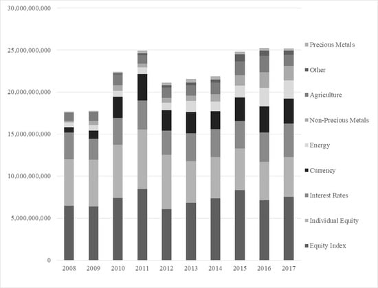
Two important components of the derivatives market are futures and options, which are widely traded all around the world. They are divided into ten groups including equity index, individual equity, interest rates, currency, energy, precious metals, non-precious metals, and agriculture.
Figure 1 depicts the volume trading over the past decade in the exchanged-traded market, showing an increase in the volume of these types of derivatives traded after the global financial crisis, from around 17.5 billion in 2008 to its peak of 25 billion in 2011. Over the next three years after its peak in 2011, the volume of exchange-trade futures and options dropped considerably, before recovering to its highest level in 2015. An increase in the volume traded after the crisis may imply that corporates or agents have turned into derivative instruments for their hedging purposes.
Among the CIJU countries, Japan and the U.S. have the most long-standing derivatives markets, with the first futures exchange set up in the Dojima Rice Exchange in Osaka, Japan, in 1730. The Chicago Board of Trade opened in the U.S. in 1848 (
Sundaram 2012). In contrast, the derivatives market in China began recently, with the opening of the China Financial Futures Exchange in Shanghai in September 2006 and later an OTC derivatives market called the Shanghai Clearing House in November 2009. However, according to a recent overview on derivatives trade in China by
Zhou (
2016), the country has one of the world’s largest commodity markets based on the amount of trade and its growth rate. The China Securities Regulatory Commission (CSRC) reported that trading on the commodity market in China has been at world levels for five years, as the cumulative volume of the future market was around
$2.5 billion and its cumulative turnover was approximately
$292 trillion. As in India, the country’s derivatives market has emerged and grown in recent years with a significantly high use of derivatives instruments. The wave of globalization and liberalization in different parts of the world made risk management more important than ever before (
Vashishtha and Kumar 2010). This view is supported by a dramatic increase in the daily turnover on the OTC, for both foreign exchange instruments and interest rate derivatives markets, as indicated in
Table 2.
4. Methodology
We address the impact of the derivatives market on economic growth and growth volatility in four economies using time-series analysis in the short and long run. First, the short-run impact was considered via the impulse response function (IRFs) through either a vector error correction model (VECM), if a long-run relationship exists, or a vector autoregression (VAR) model. The appearance of the cointegration relationship allowed us to trace the long-run effect with dynamic ordinary least squares (DOLS) and fully modified least squares (FMOLS), so that we could take the endogeneity problem into account. Second, we accessed the causal relationship between the derivatives market, macroeconomic variables, and economic growth, as well as growth volatility with the application of a causality test. Finally, based on our results, we offer policy implications for countries on the path of promoting their derivatives market, especially in emerging and developing areas with underdeveloped financial systems.
4.1. Model Specification
Based on our extensive review of the literature on financial development and economic growth as well as empirical studies on this link, we constructed an analytical framework consisting of the derivatives market, economic growth, and two macroeconomic factors, the interest rate and trade openness, which act as control variables. Our initial goal was to develop a proper procedure for estimating the link between these variables. The regression specification is as follows:
where
i and
t represent the sample country (
i = 1, …, 4) and the time series, respectively.
is the real gross domestic product (GDP) at time
t in country
i, and
is the real value of derivatives trading of exchange rate market. The nominal values of GDP and derivatives trading are converted into real terms using the consumer price index (CPI).
is the real interest rate, which is calculated by subtracting the nominal interest rate from inflation rate.
is the ratio of total exports and imports to GDP. Finally,
is the error term, and
denotes the logarithm.
A concerning issue is that the excessive development in the derivatives is associated with higher volatility in economic growth as it may increase high uncertainty in the economy. To address this issue, we incorporated the derivatives market, growth volatility, and two macroeconomic factors, the interest rate and trade openness into an integrated framework in which the growth volatility (
VOL) took the role of the economic growth as the dependent variable in Equation (1). In other words, we derived the estimated equation as follows:
where
is the volatility of real growth rate in countries
i at year
t, measured by the standard deviation of growth rate of four preceding quarters.
The study covered the four major economies in the world, namely, China, India, Japan, and the United States. The timeframe varied across countries, starting in 2006Q3 for China, 2007Q2 for India, and 1998Q1 for Japan and the U.S. Data for the analysis were collected from various sources. Information on the derivatives market originates in the Bank for International Settlements (BIS) database. It is difficult to define a good measure for the derivatives market, which has a wide variety of products. In this paper, we proxy it by total outstanding notation amounts of exchange-traded derivatives.
2 For the remaining variables, we obtained data from the International Monetary Fund (IMF) International Financial Statistics (IFS).
Table 3 describes the data for the variables.
4.2. Unit-Root Tests
To investigate how the development of the derivatives market, especially the trading of exchange rates, affects economic growth in the short and long run, we estimated Equations (1) and (2) for each individual country. Using time-series techniques, we began by testing whether the variables were stationary and whether they had a cointegrated relationship. First, to consider the stationarity, we adopted the Dickey–Fuller generalized least squares (DFGLS) unit-root test proposed by
Elliott et al. (
1996). The DFGLS test is perceived to generate better results with a small sample and has significantly greater power than the previous version of the augmented DF test. The time series was transformed via a generalized least squares (GLS) regression before the test was performed. Moreover, with the long period of about 80 quarters, the data series could exhibit structural breaks due to, for example, the dotcom crash and the 2008 global financial crisis. We also applied the ZA unit-root test by
Zivot and Andrews (
1992), which takes the existence of structural shifts in the series into account.
4.3. Cointegration Test
The next step is to examine the long-run relationship among four selected variables. The study employs the bound testing approach to cointegration by
Pesaran et al. (
2001).
3 Two proposed tests, standard
F- and
t-statistics, were performed on the basis of the conditional error correction mechanism using the autoregressive distributed lag (ARDL) model. Equations (1) and (2) is expressed in terms of the error correction version of the ARDL model as follows:
where
denotes the first difference of a variable.
The bound test cointegration consisted of two steps. First, the dependent variable was regressed on a set of regressors with the ARDL model using the ordinary least squares (OLS) technique. Before the bound test was applied in the next step, the error term should be tested to ensure it was serially uncorrelated and homoskedastic. The second step was to confirm the presence of cointegration by tracing whether all the estimated coefficients of the lag level equaled zero with the
F- and
t-statistics. That is, the
t-statistics tested the null hypothesis
against the alternative
, while the
F-statistics tested the null hypothesis
against the alternative of at least
, provided that four lags were used. If the estimated
F-statistics were smaller than the lower-bound critical value, larger than the upper-bound value, and between the lower- and upper-bound value, the null hypothesis was not rejected, rejected, and inconclusive, respectively. The lower- and upper-bound critical values are presented in
Pesaran et al. (
2001). The rejection of the null hypothesis means that a set of time series was cointegrated, implying the existence of a long-run relationship. Also, we applied the method by
Gregory and Hansen (
1996) to test for the presence of a structural break as a robustness test.
4.4. Granger-Causality Test
Equations (1) and (2) might show a causal relationship between the independent and dependent variables. A similar equation could be proposed, with each current independent variable acting as a dependent variable in turn. Therefore, we employed a causality test to clarify the direction of the variables concerned. Without the existent of the long-run link among the variables in Equations (1) and (2), we performed the traditional causality test proposed by
Engle and Granger (
1987) on the VAR model.
To investigate the uni- or bidirectional causal link between economic growth, growth volatility, and derivatives market development in view of the appearance of a long-run relationship, we depicted the Granger-causality test using a VECM framework in the following equation:
where
and
for
. The matrix
includes both the speed of adjustment to the equilibrium
and long-run information
.
For investigating the causal relationship between economic growth and derivatives markets based on Equation (1), the vector Z consists of , and for the case of growth volatility based on Equation (2), the vector Z comprises of .
The testing for Granger-causality was based on the null hypothesis that the coefficients on the lagged values of independent variables were not statistically different from zero simultaneously, using F-statistics (Wald test). In cases of the rejection of the null hypothesis, a conclusion was that the independent variable did cause the dependent variable, and both the independent and dependent variables had a stable relationship in the long run.
5. Empirical Results
5.1. Unit Root Tests and Cointegration Tests
To determine the relation between the development of a derivatives market, economic growth, and macroeconomic variables in the short- and long-run, we first checked the stationarity of all these variables. The advanced DFGLS test by
Elliott et al. (
1996) and the ZA test by
Zivot and Andrews (
1992) are performed and presented in
Table 4. The DFGLS revealed that some variables were stationary, such as the interest rate in China and trade openness in the United States while others contained unit roots. As in the DFGLS test, most variables in these four countries were found to have unit roots based on the ZA test.
4 Seven out of eight unit root tests confirmed the variable of growth volatility to be stationary at an at least 10 per cent significance level. Thus, a conclusion was that some were integrated I(0), and most series were I(1), depending on the type of stationarity test. This characteristic is quite normal for macroeconomic variables.
To consider whether the long-run relationship existed among selected variables in each country, we performed two types of cointegration tests: the ARDL bounds tests by
Pesaran et al. (
2001), and the GH test by
Gregory and Hansen (
1996) to check the sensitivity of the conclusion.
Results of the cointegration tests are shown in
Table 5. Equation (3) with the real GDP being the dependent variable is shown in Panel A while the case of growth volatility in Equation (4) is presented in Panel B. From Panel A, according to the computed
F-statistics and
t-statistics, it had a high likelihood of rejecting the null hypothesis of no cointegration at the 1 per cent significance level in China. Based on the
F-statistics, the null hypothesis was rejected in Japan, but this conclusion was not supported by the
t-statistics. In the two remaining countries (India and United States), no evidence rejected the null at even the 10% significance level. The GH tests appeared to support the findings from the ARDL bounds tests, with additional information on a structural break in each country. More specifically, a structural break was found in China and the United States in 2008, and in India and Japan in 2011 and 2013, respectively. Based on the cointegration tests, we therefore came to the conclusion that a long-run relationship among variables existed in China, but not India, Japan, and the United States. For the growth volatility, Panel B of
Table 5 illustrates that both the bound test and GH test failed to reject the null hypothesis of no cointegration for the case of China, Japan, and the United States, while India experienced the long run relationship among the growth volatility, derivatives market, trade openness, and interest rate.
5 5.2. Effect of Derivatives Market Development on Economic Growth and Volatility
With the presence of cointegration among derivatives, trade openness, and interest rate and economic growth in China, as well as growth volatility in India, we analyzed its long-run relationship further. We estimated Equation (1) for China and (2) for India using two long-run estimations, DOLS and FMOLS, and present the results in
Table 6. First, in addition to revealing the significantly positive effect on economic growth of the interest rate in the long run, these two methods showed the positive influence of the derivatives market on economic growth. Our results provided supporting evidence for an abundance of theoretical and empirical studies on the impact of the general development of financial markets to economic growth in the long run (
Ang 2008;
Beck et al. 2000;
Levine 2005;
Levine et al. 2000). In particular, our findings appear to support the theory of
Baluch and Ariff (
2007), who underline the role of liquidity level of derivatives markets in facilitating economic growth. Also,
Zhou (
2016) statistically indicates the founding and development of China’s derivative market have contributing effects to the country’s massive import, fast economic growth, and gradual maturity of financial structure. Second, we found the negative impact of the financial market on growth volatility in India. This implies that an excessive increase in the development of derivatives market can have unfavorable effects in the long run for India. The similar pattern was recorded with trade openness in India.
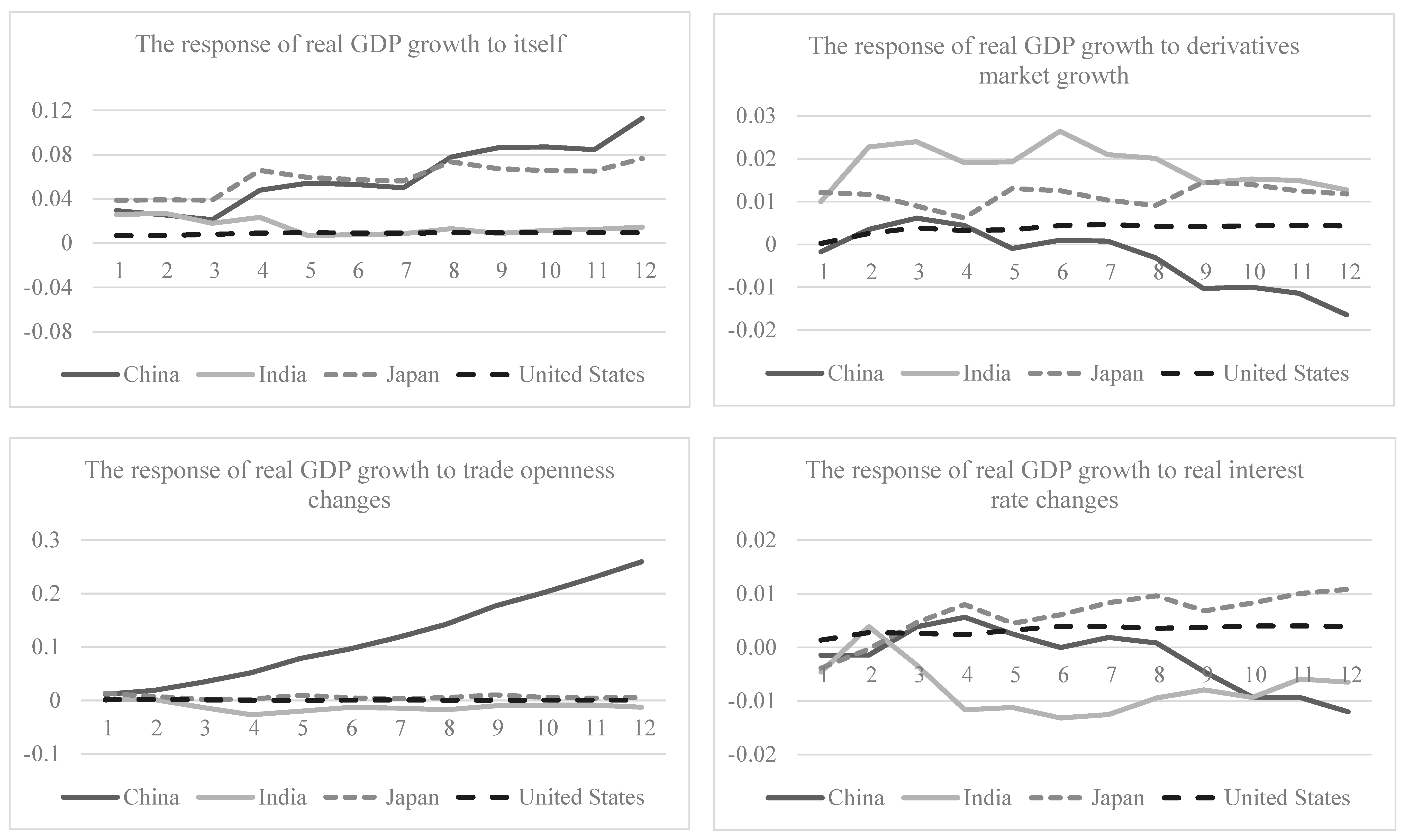
We then examined the short-run relationship among GDP growth, derivatives market development, trade openness, and the interest rate. Because of the presence of cointegration, it was better to use VECM rather than VAR. Therefore, we applied the former approach regarding China and adopt the latter method for the other countries using Equation (5), with the variables in first difference. We carried out impulse response functions (IRFs) and depict the results in
Figure 2. Graphical representations of the IRFs can illustrate the dynamic relationship, as they show the response of a variable to a shock to itself and to other variables over time. In particular, a response to GDP growth is positively affected by its own shock, with the largest magnitude experienced in China. A response to GDP growth from trade openness was much more significant in China than in the other three countries, and the response among the countries in reaction to the interest rate showed a mixed pattern. Economic growth in China tended to be positively influenced by the derivatives market in the first year but this effect turned negative over time, and the other three countries had a positive response although with a moderate magnitude.
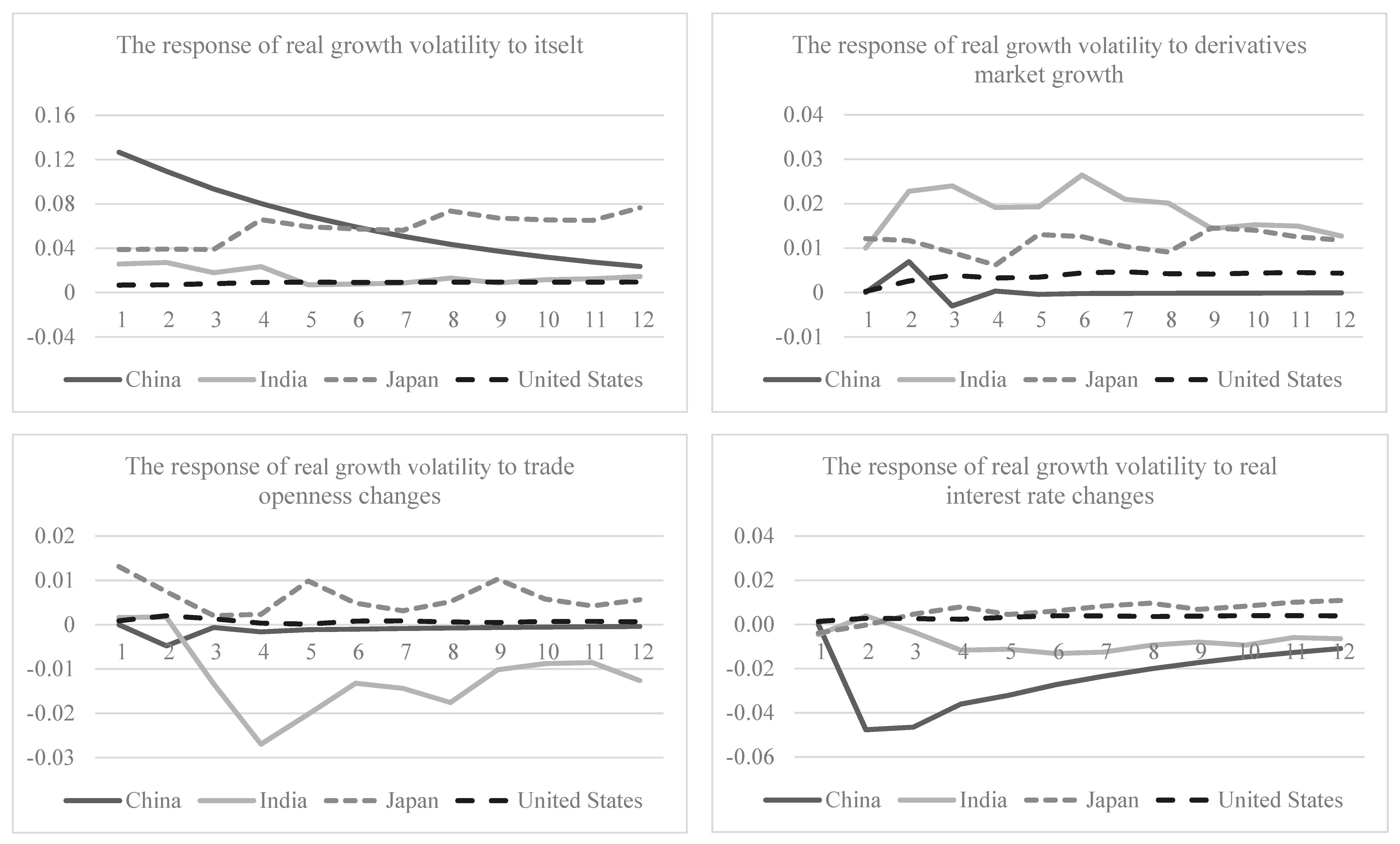
We show the IRFs for the relationship between growth volatility and other variables in
Figure 3. The IRFs were based on the VECM for the case of India and the VAR for China, Japan, and United States due to the results from the cointegration tests. Volatility shocks were recorded to be positively affected itself in China but the effect gradually declined over time while volatility in Japan had an increasingly cumulative effect by itself over the period. Shocks in the derivatives market were found to have a positive effect on the growth volatility in India and Japan, but this effect was persistent overtime. The volatility in the growth rate in United States was marginally affected by shocks in the derivatives market while no effect was found for the case of China. When it comes to the effect of the shocks of trade openness, only India experienced a negative effect associated with growth volatility and the three remaining countries had almost no effect. The similar pattern was observed for China where growth volatility was related to shocks in interest rates.
5.3. Granger Causality Effect of Derivatives Market Development on Economic Growth and Volatility
Finally, we performed a Granger-causality test to reveal any causal relations among variables. Reported in
Table 7 are the results pertaining to the model that includes economic growth with several interesting findings. First, we found no causal link between economic growth and the derivatives market in China and Japan. Meanwhile, a unidirectional impact of economic growth on the derivatives market was found in India, and the reverse was observed in the United States. Second, economic growth tended to be closely associated with trade openness, as a bidirectional causal relation was found in India and Japan, and a unidirectional impact from economic growth on trade openness was seen in Japan. Its relation with the interest rate was less significant, with a unidirectional relationship found only in Japan and China. Third, when it came to a causal relation between the derivatives markets and the two remaining variables, India had the most active reaction, as the derivatives market was found to have a bidirectional relation with the interest rate and a unidirectional impact on trade openness. Japan had a unidirectional impact on the derivatives market on both the interest rate and trade openness, whereas it was unidirectionally affected by trade openness in the United States. Our findings in relation to the causality relationship were quite different from the recent studies.
Vo et al. (
2019) show the bidirectional Granger-causality between derivatives markets and economic growth internationally using the panel vector autoregressive (PVAR) method, while
Sendeniz-Yuncu et al. (
2018) illustrate the unidirectional causality in high-income countries from economic growth to the development of a futures market, a fraction of the general derivative market.
Table 8 reports the causal relationship pertaining to the model that based on growth volatility and other variables. Generally, variables had more Granger-causal links to each other in the case of India rather than any other countries, namely, China, Japan, and United States. Specifically, India had experienced the bidirectional Granger link among growth volatility, derivatives market, and the interest rate. India had also experienced the unidirectional Granger effect from the derivatives market to growth volatility. This unfavorably potential effect empirically suggested a warning concern that the development of derivatives markets may generate an uncertainty to the domestic economy as raised by (
Haiss and Sammer 2010). In China, the interest rate was found to have a unidirectional effect on both trade openness and growth volatility. On the contrary, United States had experienced the unidirectional impact of the derivatives market and interest rate on trade openness. There was a unidirectional influence from the development in the derivatives markets on interest rate.
6. Concluding Remarks
The development of the derivatives market has played an increasingly important role in the financial market, serving not only as an effective hedging instrument but also as a useful provider of immediate information, thus boosting the efficiency of financial market operations. Recent interest focuses on how the development of derivatives markets influences the economy as a whole. Some research has theoretically suggested that the derivatives market positively affects economic growth by accelerating capital accumulation, making investment more efficient by offering more diversity in highly risky projects and reducing uncertainty in the economy as a risk hedging tool. However, insufficient empirical studies have been conducted on this important relation.
We study the relation between economic growth, volatility, and the derivatives market, as well as other macroeconomic variables: trade openness and the interest rate. We selected the four major economies (China, India, Japan, and the U.S.), which have a mature derivatives market, for our analysis using time-series econometric methods on an updated dataset up to the last quarter of 2017. The application of time-series techniques varies across countries because of the nature of the data. As such, several advanced, appropriate, and robust econometric techniques are used in this study.
The derivative market in China was found to have a significantly negative impact on economic growth in the short term, but this impact turns positive in the long run. The three remaining countries (India, Japan, and the U.S.), the results also reveal no long-run impact of the derivatives market on economic growth, but a positive impact was found in the short run. Moreover, the causality test indicates that India has a unidirectional effect from the derivatives market to economic growth whereas the reverse pattern is observed in the U.S., and no causality effect was found between these two variables in China and Japan. Also, India had experienced the bidirectional causal relationship India among growth volatility, the derivatives markets, and the interest rate.
We concluded that development of the derivatives markets had a positive effect on economic growth in the short run, as indicated in India, Japan, and the U.S., although it may gradually turn negative, as in China. However, it was found to generate an unexpected effect on growth volatility in India. In light of these findings, this research supports the theory on the favorable effect of the derivatives market on economic growth. As such, we suggest that any strategy for enhancing or boosting the size of the derivatives market should be encouraged, especially in emerging and developing countries so as to boost economic development, although it is important to have a proper regulatory framework in order to prevent unintended consequences, such as creating a negative impact in the short run as seen in China, causing the growth volatility as observed in India.
A limitation of the current paper is that the sample sizes including four selected countries covered approximately 80 observations and the applications of VAR or VECM required time lags for all variables, leading to a significant reduction of the number of the degrees of freedom. As a consequence, it raised a concern in relation to the biased coefficients in the estimation. In our future studies, a more comprehensive inclusion of dynamic panel data models, unit root tests, or cointegration analysis will be applied to ensure that empirical findings are more robust.


