Growth and Debt: An Endogenous Smooth Coefficient Approach

Abstract

The new growth theories with an emphasis on fundamental determinants such as institutions suggest a non-linear cross-country growth process. In this paper, we investigate the public debt and economic growth relationship using the semi-parametric smooth coefficient approach that allows democracy to influence this relationship and parameter heterogeneity in the unknown functional form and addresses the endogeneity of variables. We find results consistent with the previous literature that identified a significant adverse effect of public debt on growth for the countries below a particular democracy level. However, we also find conclusive evidence that countries with high institutional quality have an adverse effect of public debt on growth for the period 1980–2009, as well as for the extended period including the years 2010–2014. A 10-percentage point increase in the debt-to-GDP ratio is associated with a 0.12% and 0.07% decrease in the subsequent 10-year period real GDP growth rate for the zero democracy countries and for the countries with a democracy score of 10, respectively.

1. Introduction

In the aftermath of the recent global financial crisis, government debt has increased substantially across the world. For advanced economies, the public debt-to-GDP ratio rose on average from about 66% in 2007 to 105% by the end of 2015. Particularly, Greece, Ireland, Japan, Portugal, Spain, and the United Kingdom, when compared to other countries, experienced a rapid and higher increase in public debt-to-GDP ratio between 2008 and 2012. A growing concern behind these facts is that countries may not achieve debt sustainability, implying higher vulnerability to an economic and financial crisis (Cecchetti et al. (2010); Bohn (1995)). In fact, over the last two centuries, there were twenty financial crises followed by debt build-up periods, which lasted more than a decade and are associated with lower growth than during other periods (Reinhart et al. (2012)). Therefore, a relevant policy question centers on the long-term growth effects of high public debt.

The relationship between public debt and economic growth is still unresolved in both the theoretical and empirical literature. Theoretically, the conventional view of public debt is that fiscal deficits in the short-run can have a positive effect on economic growth by stimulating aggregate demand and output, whereas it also may have a potential crowding out effect on private investment in the long run (Elmendorf and Mankiw (1999)). On the other hand, much of the economic growth literature reveals some evidence of nonlinearity in the effect of public debt on growth, mainly focusing on threshold levels. The idea is to detect a debt level beyond which economic growth is adversely affected, implying a concave (inverted-U shape) relationship between debt and growth. Using a basic nonparametric technique (i.e., a histogram, to investigate a correlation between public debt and growth), Reinhart and Rogoff (2010) found a threshold level of 90% for 20 advanced countries between 1945 and 2009. Their findings are striking in that an average of real GDP growth decreases substantially (at about 4%) when public debt-to-GDP ratio is beyond the 90% threshold as compared to other public debt-to-GDP ratios. Moreover, the debt-growth link disappears for the public debt ratios below the 90% threshold.

In the empirical growth literature, an extensive number of studies have tried to examine the sensitivity of Reinhart and Rogoff’s 90% threshold level to model specifications, alternative sets of included and excluded variables, and different data series.

Table A1. Summary statistics.

	Mean	Std. Dev.	Min	Max
Panel A. Penn World Table 7.0 (1980–2009)
Growth	0.014	0.023	−0.099	0.083
Initial income	8.42	1.27	5.87	10.71
Lag of initial income	8.34	1.23	5.78	10.55
Investment rate	3.05	0.35	1.87	3.89
Lag of investment rate	3.05	0.39	1.74	4.31
Population growth rate	−2.71	0.16	−3.23	−2.38
Lag of population growth rate	−2.69	0.16	−3.08	−2.28
Government consumption	2.19	0.44	1.06	3.56
Lag of government consumption	2.19	0.48	1.01	3.69
Trade openness	66.51	36.49	9.77	199.86
Lag of trade openness	61.01	35.80	9.70	180.09
Panel B. Penn World Table 9.0 (1980–2014)
Growth	0.025	0.029	−0.061	0.114
Initial income	8.77	1.17	6.42	11.20
Investment rate	2.96	0.45	0.65	3.92
Population growth rate	−2.71	0.15	−3.07	−2.38
Schooling	0.77	0.32	0.036	1.31
Panel C. World Bank
Inflation rate	2.30	1.17	−1.95	7.57
Lag of inflation rate	2.34	1.19	−1.46	8.26
Life expectancy	4.17	0.17	3.63	4.41
Lag of life expectancy	4.14	0.18	3.63	4.38
Fertility	3.62	1.73	1.21	7.78
Lag of fertility	4.06	1.89	1.17	7.82
Panel D. IMF
Public debt	4.08	0.61	2.17	6.33
Lag of public debt	3.92	0.73	1.12	6.46
Panel E. Barro and Lee (2000)
Schooling	0.60	0.77	−2.18	1.97
Lag of schooling	0.32	0.90	−2.66	1.90
Panel F. Polity IV
Democracy	5.74	3.83	0.00	10.00
Lag of democracy	5.02	4.17	0.00	10.00
Executive constraints	4.96	2.05	1.00	7.00
Lag of executive constraints	4.51	2.33	1.00	7.00
Panel G. Freedom House
Political rights	4.82	1.93	1.00	7.00
Lag of political rights	4.53	2.08	1.00	7.00
Civil liberties	4.67	1.68	1.00	7.00
Lag of civil liberties	4.45	1.77	1.00	7.00

in the Appendix A provides a summary of recent studies aimed at unveiling the nonlinear relationship between government debt and economic growth. An important observation gleaned from this table is that there is no common finding for the threshold level, except for a small number of studies that found a turning point for a public debt-to-GDP ratio at around 90%. In one study in the latter group of papers, Cecchetti et al. (2011) examined a panel of 18 OECD countries (all from advanced economies) for the period 1980–2006. Using least squares dummy variables threshold estimation within the context of the dynamic fixed-effects panel data model, they found a negative relationship between government debt and growth beyond the 85% threshold level after controlling for other determinants of growth including trade openness, inflation rate, and total dependency ratio (related to aging). Their approach avoided a possible feedback effect from economic growth to public debt by using five-year averages of growth, so that regressors were predetermined. Their results suggest that, on average, a ten-percentage points increase in the debt-to-GDP ratio is predicted to reduce economic growth by 0.13 percentage points per year. In Checherita-Westphal and Rother (2012), a study of 12-Euro area economies from 1970–2008, they aimed to investigate nonlinearity in the debt-growth link by using a quadratic equation in debt. To control for endogeneity of the public debt variable, the authors used a lagged value of debt and average debt of the other countries in the sample. They found a public debt threshold level between 90% and 100%, beyond which economic growth was negatively affected. Baum et al. (2013) dealt with the endogeneity problem arising from the dynamic model specification in their study of 12-Euro area countries from 1990–2007 and 2010. They found a threshold level of the public debt-to-GDP ratio at 95% for the extended period. In another study, Woo and Kumar (2015) surveyed 38 advanced and emerging economies from 1970–2008. Using several estimation strategies and subsamples, the authors examined non-linearity in the debt-growth relationship by fitting the data to the dynamic panel regression model. They also found a 90% threshold level beyond which public debt had a negative and significant effect on economic growth. Panizza and Presbitero (2014) accounted for the potential endogeneity of public debt using the share of foreign currency debt in total public debt as an instrument. Using the same dataset and empirical approach of Cecchetti et al. (2011), as well as performing various robustness checks, they found little evidence of the adverse effect of high public debt on future growth in advanced economies.

Other studies provide evidence of a threshold level of public debt different from 90% of GDP. For example, Caner et al. (2010) studied a cross-section of 101 developed and emerging market economies from 1980–2008. Using threshold estimation, they found a turning point of the public debt-to-GDP ratio at 77% for the full sample controlling for initial GDP per capita, trade openness, and inflation rate; this value was lower at 64% of GDP for the subsample of developing countries. In the Wright and Grenade (2014) study of 13 Caribbean countries from 1990–2012, the authors found a threshold level of 61% of GDP beyond which debt had a negative effect on economic growth and investment. Some research studies closely replicated the research of Reinhart and Rogoff (2010) using different econometric techniques. For example, Minea and Parent (2012) employed the panel smooth transition regression model of Gonzáles et al. (2005) and found an adverse and gradually decreasing effect of public debt on growth below the threshold level of 115%. Their finding supported the presence of nonlinearity in the effect of debt on growth for the debt-to-GDP ratio above 90%. On the other hand, they found a positive growth effect of debt for the debt level above 115%. In a related study, using nonlinear threshold models for the same dataset used in Reinhart and Rogoff (2010), Égert (2015) found limited evidence for a negative nonlinear correlation between public debt and growth. The author’s findings suggest that a debt threshold level can be lower than 90% of GDP depending on data coverage (regarding country coverage and time dimension), model specification, and different measures of the public debt. Eberhardt and Presbitero (2015) provided strong evidence of different non-linearities in the debt-growth relationship across 118 countries from 1961–2012 by doing a comprehensive analysis of dynamic panel time series estimation (see Eberhardt and Presbitero (2013) for the earlier version of the authors’ work). They employed a common factor framework to uncover possible heterogeneity in the effect of public debt stock on economic growth by considering latent factors of growth and public debt, which include a country’s debt composition, macroeconomic policies related to past crises, and institutional framework. They found no evidence for the common threshold effect for all countries in their sample.

A primary purpose of the above-discussed research studies was to reveal a nonlinear relationship between public debt and economic growth depending on the public debt level. In other words, these researchers tried to expose the nonlinear growth effect of high public debt levels. However, this point of view ignores potential variables, either omitted from the model or included as a regressor, that may govern the debt-growth relationship. This concern raises an important question: Is the high public debt a primary source of the negative relationship between debt and growth? Kourtellos et al. (2013) studied 82 countries in a 10-year panel from 1980–2009 to test formally for several threshold variables including democracy, trade openness, fertility, life expectancy, and inflation rate, among others. They employed the structural threshold regression model of Kourtellos et al. (2016) to account for the endogeneity of both the threshold variable and the regressors. The authors found strong evidence in favor of heterogeneity in the debt-growth relationship in the sense that the effect of public debt on economic growth depends on the institutional quality of a country. Notably, they found that, holding other factors fixed, countries with low institutional quality experienced a negative and significant effect of public debt on economic growth, while public debt had a positive, but insignificant effect on growth for countries with high institutional quality. Jalles (2011) investigated the impact of democracy and corruption on the external debt-growth relationship in a panel of 72 developing countries from 1970–2005. Using fixed effects and GMM estimation strategies under various model specifications (linear and quadratic terms in debt-to-GDP ratio), the author found a negative growth effect of external debt in countries with higher levels of corruption. These findings are consistent with the such new growth theories as the suggestion of Azariadis and Drazen (1990) of a highly nonlinear cross-country growth process (see also Temple (1999) for further reading).

Institutional differences across countries are perceived as one of the primary factors in the cross-country income gap. In a seminal paper by Acemoglu et al. (2001), the authors documented a positive relationship between democracy and per capita GDP after controlling for the endogeneity of institutions from an exogenous source of variation (see also Acemoglu et al. (2015) for recent work on the same subject). Another argument is that the democracy variable is not correctly measured as many institutional measures reflect the outcome of dictatorial choices and, therefore, should be seen as institutional outcome variables, not predictors of it (see, for example, Glaeser et al. (2004) and Acemoglu et al. (2005)). On the other hand, Minier (2007) examined democracy as a source of heterogeneity in the relationship between economic growth and its determinants, and the author provided some evidence of an indirect effect of institutions regarding the link between trade openness and economic growth.

Given that the relationship between public debt and growth appears to be heterogeneous and complex and there may be other factors that contribute to the marginal impacts of variables on economic growth, our aim in this paper is to examine whether democracy may influence the relationship between public debt and economic growth in our sample of countries. The limitations of the existing debt-growth literature coupled with the lack of explicit theoretical argument on the debt-growth link in advanced economies suggests that a flexible approach may be more appropriate for estimating the effect of debt on growth and seeking other factors to characterize this relationship. We, therefore, present an augmented conventional Solow economic growth model with public debt-to-GDP ratio and country-specific parameters, which relax the homogeneity assumption of a standard growth regression. Specifically, as a first assumption, we model parameters to be a function of one or more covariates including democracy, fertility, and life expectancy, among others. Our approach is also related to the empirical growth studies that use nonparametric and semiparametric models to model parameter heterogeneity in the cross-country growth process. Examples include Liu and Stengos (1999) and Ketteni et al. (2007) for an additive semiparametric partially linear model; Vaona and Schiavo (2007) for a semiparametric partial linear model; Durlauf et al. (2001), Mamuneas et al. (2006), Kourtellos (2011), and Kumbhakar and Sun (2012) for a varying coefficient model; and Henderson et al. (2011) for a nonparametric model.

To ensure that our regression model captures the heterogeneous effects of variables, we further assume the parameters to be unknown measurable smooth functions. This assumption enables us to use nonparametric techniques, which essentially allows the data to decide the functional form of each parameter. Moreover, the coefficient estimates avoid bias by the misspecification of parameter heterogeneity, which occurs in a parametric form in the existing debt-growth studies. Furthermore, economic theory does not suggest a functional form for the regression model of debt-growth relationship or even for the parameter heterogeneity in the debt-growth link. Therefore, nonparametric techniques permit unknown functions to be governed by country-specific characteristics such as the country’s initial conditions, state of development variables, institutional quality, and macroeconomic policies playing an indirect role in explaining a nonlinear relationship between growth and its determinants across countries and the time domain. For this study, we used a recently-developed smooth coefficient instrumental variable estimator of Delgado et al. (2015) that assumes linearity in the regressors, but allows the intercept and slope coefficients to be an unknown function of a covariate (e.g., democracy). Moreover, with this estimator, we can control for endogeneity of a covariate in the unknown functional coefficients.

We fit the semiparametric smooth coefficient model to a dataset including 82 countries for the three 10-year averages spanning from 1980–2009. We also extend this dataset by adding recent years from 2010–2014 for 78 countries. We find strong evidence of heterogeneity in the effect of public debt with respect to institutional quality of countries. Additionally, we find conclusive evidence in support of the recently shifted focus in the debt-growth relationship that institutions may be one of the factors that influence this relationship. Specifically, our results are consistent with the literature that identified an average negative and statistically-significant effect of public debt on growth. However, our empirical results also show that for high democracy countries, a higher debt-to-GDP ratio leads to lower economic growth where everything else is equal. Our core results suggest that a ten percentage point increase in the debt-to-GDP ratio is associated with a 0.12% (and 0.071%) decrease in the subsequent ten-year period real GDP growth rate for zero democracy countries (and for the countries with a democracy score of 10).

Our findings are robust to different measures of democracy, different country groupings, and to the inclusion of additional control variables. Our results from prediction exercises also suggest that our semiparametric model can better describe the underlying process that generated the data than the parametric models. We, therefore, are contributing to the empirical debt-growth literature by explaining parameter heterogeneity in the cross-country growth process through fundamental determinants of economic growth proposed by new growth theories.

The remainder of this paper is organized as follows. Section 2 describes our empirical methodology. Section 3 describes our data. Section 4 presents the empirical results of the study. Section 5 presents our robustness checks. Section 6 presents the conclusion.

2. Empirical Methodology

2.1. The Augmented Solow Growth Model

In this section, we provide a brief description of a linear Solow growth model augmented with the debt-to-GDP ratio to investigate the impact of country’s debt level on its economic growth rate. This model assumes a common regression across countries, as well as constant coefficient estimates for all economic variables, which intuitively explains the average effect of the variables.

$$g_i=X_i^T\beta +u_i={\beta }_0+S_i^T{\beta }_s+{\beta }_{d}deb{t}_i+u_i,i=1,\dots ,n,$$

(1)

where $X_i={[1,S_i^T,deb{t}_i]}^T$ is a $(d_s+2)\times 1$ vector of regressors consisting of a constant term, a $d_s$-dimensional vector of standard Solow growth determinants, including $ln\left(yi{n}_i\right)$, the logarithm of the $i^{\mathrm{th}}$ country’s real GDP per worker in the initial year of each 10-year period; $ln\left(s_i\right)$, the logarithm of the $i^{\mathrm{th}}$ country’s average saving rate; $ln(n_i+0.05)$, the logarithm of the $i^{\mathrm{th}}$ country’s population growth plus 0.05; $ln\left(sc{h}_i\right)$, the logarithm of the $i^{\mathrm{th}}$ country’s average years of secondary and tertiary schooling for the male population over 25 years of age; and $deb{t}_i$, which is defined as the $i^{\mathrm{th}}$ country’s public debt-to-GDP ratio. Moreover, $S_i$ includes a time trend. $u_i$ is an identically and independently distributed error term.

2.2. An Endogenous Smooth Coefficient Model

We consider the following semiparametric varying coefficient model of Delgado et al. (2015) for the augmented Solow growth model:

$$\left\{\begin{array}{c}{g}_i={\theta }_0\left(Z_i\right)+{\sum }_{j=1}^{d_s}{\theta }_{sj}\left(Z_i\right)S_{ji}+{\theta }_d\left(Z_i\right)deb{t}_i+{ϵ}_i\hfill \\ Z_i={\mu }_Z+a_1\left(E_{i,1}\right)+a_2\left(E_{i,2}\right)+\dots +a_p\left(E_{i,p}\right)+u_i,i=1,\dots ,n,\hfill \end{array}\right.$$

(2)

$$\left(i\right)E\left[u_i\right|{\mathit{E}}_{\mathit{i}}]=0$$

$$\left(ii\right)E\left[{ϵ}_i\right|{\mathit{E}}_{\mathit{i}},u_i]=E\left[{ϵ}_i\right|u_i],i=1,\dots ,n,$$

where $Z_i$ is an endogenous variable defined as an additive nonparametric function of $E_{ij}$, $j=1,\dots ,p$, where ${\mathit{E}}_{\mathit{i}}=[E_{i,1},E_{i,2},\dots ,E_{i,p}]={[S_i^T,deb{t}_i,W_i^T]}^T$ is a $p\times 1$ vector of continuous variables including a $d_w$-dimensional vector of instrumental variables, $W_i^T$. $a_t(·)$, $t=1,\dots ,p$, ${\theta }_0(·),{\theta }_s(·)$, ${\theta }_d(·)$ are all unknown smooth measurable functions, and $u_i$ is a zero-mean error term.

In Equation (2), the object of estimation is the structural model that necessitates different identification strategies than standard nonparametric regression, which is used to estimate conditional expectations. The additive separability of Z and the conditional mean of $ϵ$ and u given in (i) and (ii) in Equation (2) are nonparametric restrictions for identification in this model.1

After setting $E\left[{ϵ}_i\right|u_i]\equiv b\left(u_i\right)$ and denoting $v_i\equiv {ϵ}_i-b\left(u_i\right)$, which satisfies $E\left[v_i\right|{\mathit{E}}_{\mathit{i}},u_i]=0$, we can rewrite Model (2) as:

$$g_i={\theta }_0\left(Z_i\right)+\sum _{j=1}^{d_s}{\theta }_{sj}\left(Z_i\right)S_{ji}+{\theta }_d\left(Z_i\right)deb{t}_i+b\left(u_i\right)+v_i,i=1,\dots ,n,$$

(3)

provided that $b(·)$ is an unknown smooth function. Equation (3) consists of two additive components, ${\theta }_0\left(Z_i\right)$ and $b\left(u_i\right)$, together with the functional coefficient terms, ${\sum }_{j=1}^{d_s}{\theta }_{sj}\left(Z_i\right)S_{ji}$ and ${\theta }_d\left(Z_i\right)deb{t}_i$. According to Newey et al. (1999), identification of unknown functions in Equation (3) is the same as identification in Equation (2), as the additive structure of Equation (3) is equivalent to conditional mean restriction (Assumption (ii)) in Equation (2). The sufficient condition for identification of unknown functions in Equation (3) is, therefore, assuming no additive functional relationship between $Z_i$ and $u_i$ (see Newey et al. (1999), Theorems 2.1 and 2.2 on pp. 567–68).

If we assume that Z and all conditioning variables are exogenous, then the first equation in (2) is a pure varying coefficient model that can be consistently estimated using the nonparametric kernel estimator of Li et al. (2002); otherwise, this estimator yields a bias in estimation of unknown functional coefficients. Assuming the exogeneity of covariates seems to be strong in the present growth application; we, therefore, allow variables representing Z to be endogenous. This endogeneity assumption is that growth regression is formulated as in the structural form of Model (2), called a triangular nonparametric simultaneous equations model.

Nonparametric estimators for regression models that include endogeneity problem have been proposed in the context of varying coefficient models, for example Das (2005), Cai et al. (2006), and Cai and Li (2008). However, these papers allow for endogenous variables in the parametric part of a regression. The estimator proposed by Delgado et al. (2015), on the other hand, deals with endogenous variables that appear in the nonparametric part of a smooth coefficient model. This estimator is applicable to the economic studies, where the endogenous variable has a potential interaction effect with the other regressors on the response variable. For example, child care use may have a potential indirect effect on students’ test scores that can be modeled as in the functional coefficient form that varies with respect to mother’s education, age, and experience, among other regressors (see Bernal and Keane (2011) for a parametric estimation and full description of the regressors and Ozabaci et al. (2014) for an additive nonparametric regression estimation).

To circumvent the endogeneity problem, Delgado et al. (2015) used the control function approach in the estimation of the structural function of interest. Since u enters Equation (3) as a conditioning variable and it is generally unobserved, Delgado et al. (2015), first, calculated $\widehat{u}$ from the regression of Z on ${\mathit{E}}_{\mathit{i}}$ using the second equation of Model (2). Then, they estimated $\theta \left(Z_i\right)$ and $b\left(\widehat{u}\right)$ via the sieve approximation approach by an ordinary least squares method. In the third step, they used a local linear regression method to estimate $\theta \left(Z_i\right)$ and ${\theta }^{\prime }\left(Z_i\right)$. They showed that their estimator was oracle efficient in the sense that large sample distribution of the estimator was the same regardless of whether the function $b(·)$ was known. It is also noted that the third-step estimator is not affected by the errors in the first two steps of estimation. The estimation procedure is given in detail as follows.

In the first step, Delgado et al. (2015) approximated unknown functions $a_1(·)$, …, $a_p(·)$ by series expansions2:

$$a_m^{*}\left(e\right)=\sum _{l=1}^{L_n}{\alpha }_{ml}{\varphi }_l\left(e\right),$$

(4)

for $m=1,\dots ,p$, where ${\alpha }_m={({\alpha }_{m1},{\alpha }_{m2},\dots ,{\alpha }_{m{L}_n})}^T$ is an $L_n\times 1$ vector of unknown coefficients, ${\left\{{\varphi }_j(·)\right\}}_{j=1}^{L_n}$ is a sequence of square integrable orthonormal basis functions over the interval $[0,\infty )$, and $L_n$ denotes the number of basis functions. It is noteworthy that the Laguerre polynomial series is used to approximate the unknown functions, as it is one of the common choices for series expansions when a function has a domain over $[0,\infty )$ (see, e.g., Assumption 1(ii) in Delgado et al. (2015) and Chen (2007) for further details).

The coefficients ${\alpha }_m$, $m=1,\dots ,p$ in (4) can be consistently estimated from the ordinary least squares (or OLS) regression of $Z_i$ on $a_1^{*}\left(E_{i,1}\right),a_2^{*}\left(E_{i,2}\right),\dots ,a_p^{*}\left(E_{i,p}\right)$. Then, the OLS estimator of the unknown function is given by ${\widehat{a}}_m\left(e\right)={\sum }_{l=1}^{L_n}{\widehat{\alpha }}_{ml}{\varphi }_l\left(e\right)$, $m=1,\dots ,p$. Fitted values and the residuals from the OLS regression can be calculated as ${\widehat{Z}}_i=\widehat{\mu }+{\widehat{a}}_1\left(E_{i,1}\right)+{\widehat{a}}_2\left(E_{i,2}\right)+\dots +{\widehat{a}}_p\left(E_{i,p}\right)$ and ${\widehat{ϵ}}_i=Z_i-{\widehat{Z}}_i$ for all $i=1,\dots ,n$, respectively.

In the second step, using series expansions, they approximate unknown functions $\theta \left(z\right)$ and $b\left({\widehat{ϵ}}_i\right)$, respectively, by:

$${\theta }_k^{*}\left(z\right)=\sum _{l=1}^{L_n}{\beta }_{kl}{\varphi }_l\left(z\right),\mathrm{and}{b}^{*}\left(\widehat{ϵ}\right)=\sum _{l=1}^{L_n}{\gamma }_l{\varphi }_l\left(\widehat{ϵ}\right),$$

(5)

where ${\beta }_k={({\beta }_{k1},{\beta }_{k2},\dots ,{\beta }_{k{L}_n})}^T$ for $k=0,\dots ,d_s+1$, and $\gamma ={({\gamma }_1,{\gamma }_2,\dots ,{\gamma }_{L_n})}^T$ are all $L_n\times 1$ vectors of unknown coefficients. Model (3) can be, now, approximated by substituting equalities in (5) for ${\theta }_k\left(z\right)$, $k=0,\dots ,d_s+1$, and $b\left(\widehat{ϵ}\right)$ in Model (3).

$$g_i\approx \sum _{k=0}^{d_s+1}\sum _{l=1}^{L_n}{\beta }_{kl}{\varphi }_l\left(z\right)X_{ki}+\sum _{l=1}^{L_n}{\gamma }_l{\varphi }_l\left({\widehat{ϵ}}_i\right)+v_i,i=1,\dots ,n,$$

(6)

where residual ${\widehat{ϵ}}_i$ is calculated from the first step. The least squares problem is, then, defined as follows:

$${[{\widehat{\beta }}^T,{\widehat{\gamma }}^T]}^T=\arg \underset{(\beta ,\gamma )}{min}\sum _{i=1}^n{\left\{g_i-\sum _{k=0}^{d_s+1}\sum _{l=1}^{L_n}{\beta }_{kl}{\varphi }_l\left(z\right)X_{ki}+\sum _{l=1}^{L_n}{\gamma }_l{\varphi }_l\left({\widehat{ϵ}}_i\right)\right\}}^2.$$

(7)

In the third step, Delgado et al. (2015) used the local linear regression approach to estimate the functional coefficients, $\theta (·)$, and its first-order derivatives, ${\theta }^{\prime }(·)$. Following Delgado et al. (2015), we assume that the unknown function, $\theta \left(Z\right)$, is continuously differentiable up to second order, so that we can apply a first order Taylor series approximation of $\theta \left(Z\right)$ around a given point z, technically by $\theta \left(Z\right)\approx \theta \left(z\right)+{\theta }^{\prime }\left(z\right)(Z-z)$. We, further, assume $K(·)$ to be a kernel weight function assigning more weights to the observations closer to point z, satisfying: (i) $\int K\left(a\right)da=1$, (ii) K(a) = K(−a), and (iii) $\int a^{2}K\left(a\right)da>0$. In the case of the higher dimensional covariate vector, Z, which includes continuous and discrete covariates, the kernel function is the product kernel, $K=WL(Z^d,z^d,\lambda )$, where $W=W((Z^c-z^c)/h)$, $Z^c$ is the continuous covariate, $L_{\lambda }$ is the kernel function for the discrete variable, $Z^d$, and $\lambda$ is the smoothing parameter for the discrete covariate; see Racine and Li (2004) for further details about kernel functions for the categorical variables. We use a single continuous covariate in the kernel function given in (8).

Replacing $b\left({ϵ}_i\right)$ in Equation (3) by $\widehat{b}\left({\widehat{ϵ}}_i\right)$ calculated from the second-step estimation and treating ${\widehat{g}}_i=g_i-\widehat{b}\left({\widehat{ϵ}}_i\right)$ as a dependent variable, Delgado et al. (2015) showed that a consistent estimate of $(\theta (·),{\theta }^{\prime }(·))$ can be obtained from a minimization of a kernel-weighted objective function:

$$\underset{\theta \left(z\right),{\theta }^{\prime }\left(z\right)}{min}\sum _{i=1}^n{[{\widehat{g}}_i-X_i^T\theta \left(z\right)-X_i^T{\theta }^{\prime }\left(z\right)(Z_i-z)]}^{2}K((Z_i-z)/h),$$

(8)

where ${\theta }^{\prime }\left(z\right)$ reflects the partial effects $\partial \theta \left(z\right)/\partial z$ and h is the bandwidth controlling the size of the local neighborhood around an interior point z.

Letting $\delta \left(z\right)=[\theta \left(z\right),{\theta }^{\prime }\left(z\right)]$, the solution of Problem (8) is given by:

$$\tilde{\delta }\left(z\right)={\left({\mathbf{X}}^T\mathbf{K}\mathbf{X}\right)}^{-1}{\mathbf{X}}^T\mathbf{K}\widehat{g},$$

(9)

where $\mathbf{X}$ is an $n\times 2(d_s+2)$ matrix having $(X_i^T,X_i^T(Z_i-z))$ as its $i^{\mathrm{th}}$ row and $\mathbf{K}$ is a $n\times n$ diagonal matrix with the $i^{\mathrm{th}}$ diagonal element being $K((Z_i-z)/h)$.

The bandwidth parameter has a particular importance in the estimation of non-/semiparametric models as it determines the degree of smoothing. We use a cross-validation method, a data-driven approach, to choose the bandwidth parameter so that the bias-variance trade-off in the estimation is optimized by using the data themselves. We also provide wild-bootstrap standard errors, which are robust to heteroscedasticity, using 399 bootstrap replications Härdle and Marron (1991).

We use three goodness-of-fit measures including in-sample $R^2$, out-of-sample $R^2$, and average squared predicted error (ASPE). The out-of-sample measures are robust to over-fitting of the model, which, therefore, implies that the model of interest may better describe the underlying process that generated the data. The predictive exercises are based on 1000 bootstrap replications. We use 80 percent of the data to estimate the model parameters and evaluate on the hold-out data; see Henderson and Parmeter (2015).

3. Data

We employ the same dataset as used in Kourtellos et al. (2013) to investigate the long-run growth effect of public debt. We provide the source and definition of each variable in

Table A3. List of countries grouped into coefficient estimates from SPSCM-IVand democracy score from the Polity IV dataset.

	Negative and Significant		Insignificant
≤1	≥7.6 & ≤9	≥9
Algeria (1980, 1990)	Argentina (2000)	Australia (1980, 1990, 2000)	Argentina (1980, 1990)
Bangladesh (1980)	Bolivia (1990, 2000)	Austria (1980, 1990, 2000)	Benin (1990, 2000)
Benin (1980)	Botswana (2000)	Belgium (1980, 1990, 2000)	Bangladesh (1990, 2000)
Burundi (1980, 1990)	Brazil (1990, 2000)	Canada (1980, 1990, 2000)	Bolivia (1980)
Cameroon (1980, 1990, 2000)	Chile (1990, 2000)	Costa Rica (1980, 1990, 2000)	Botswana (1980, 1990)
Central African Republic (1980)	Colombia (1980, 1990)	Cyprus (1980, 1990, 2000)	Brazil (1980)
Chile (1980)	Dominican Republic (2000)	Denmark (1980, 1990, 2000)	Burundi (2000)
Cote’d Ivoire (1980, 1990)	Ecuador (1980, 1990)	Finland (1980, 1990, 2000)	Central African Republic (1990, 2000)
Egypt (1980, 1990, 2000)	France (1980)	France (1990, 2000)	Congo Republic (1990)
Gabon (1980, 1990, 2000)	Greece (1980)	Greece (1990, 2000)	Cote’d Ivoire (2000)
Gambia (2000)	Guatemala (2000)	Ireland (1980, 1990, 2000)	Colombia (2000)
Ghana (1980)	India (1980, 1990, 2000)	Italy (1980, 1990, 2000)	Dominican Republic (2000)
Guyana (1980)	Republic of Korea (2000)	Israel (1980, 1990, 2000)	Ecuador (2000)
Indonesia (1980, 1990)	Lesotho (2000)	Jamaica (1980, 1990, 2000)	Gambia (1980, 1990)
Iran (1980)	Mexico (2000)	Japan (1980, 1990, 2000)	Ghana (1980, 1990)
Kenya (1980, 1900)	Panama (1990, 2000)	Netherlands (1980, 1990, 2000)	Guatemala (1990)
Lesotho (1980)	Paraguay (2000)	New Zealand (1980, 1990, 2000)	Guyana (1990, 2000)
Malawi (1980)	Peru (2000)	Norway (1980, 1990, 2000)	Honduras (1980, 1990, 2000)
Mali (1980)	Philippines (2000)	Portugal (1980, 1990, 2000)	Kenya (2000)
Mauritania (1980, 2000)	Senegal (2000)	Spain (1980, 1990, 2000)	Lesotho (1990)
Morocco (1980, 1990, 2000)	South Africa (1990, 2000)	Sweden (1980, 1990, 2000)	Malaysia (1980, 2000)
Nicaragua (1980, 1990)	Thailand (1990)	United Kingdom (1980, 1990, 2000)	Malawi (1990, 2000)
Niger (1980)	Trinidad & Tobago (1990, 2000)	United States (1980, 1990, 2000)	Mali (1990, 2000)
Panama (1980)	Turkey (1990, 2000)	Uruguay (1990, 2000)	Mexico (1980, 1990)
Paraguay (1980)	Venezuela (1980, 1990)		Nepal (1980, 1990, 2000)
Sierra Leone (1980)			Nicaragua (1990)
Swaziland (1980, 1990, 2000)			Niger (1990, 2000)
Syria (1980, 1990, 2000)			Pakistan (1980, 1990, 2000)
Togo (1980, 1990, 2000)			Papua New Guinea (1980, 1990, 2000)
Tunisia (1980, 1990, 2000)			Paraguay (1990)
Zambia (1980)			Republic of Korea (1980, 1990)
Zimbabwe (1990)			Peru (1980, 1990)
			Sierra Leone (1980, 2000)
			South Africa (1980)
			Sri Lanka (1980, 1990, 2000)
			Thailand (2000)
			Turkey (1980)
			Venezuela (2000)
			Zambia (1990, 2000)
			Zimbabwe (1980, 2000)

in the Appendix A. We have a balanced 10-year period panel dataset covering 82 countries from 1980–1989, 1990–1999, and 2000–2009. Working with 10-year averages allows us to avoid any short-run fluctuations in macroeconomic variables. We also obtain an extended dataset and construct 10-year and five-year averages for a sample of 78 countries using the latest version of Penn World Table (PWT 9.0).3

We use the per capita real GDP growth rate as a measure of economic growth. We include traditional Solow regressors as control variables in our model. These variables are the initial level of income at the beginning of each ten-year period, which is expected to be negatively related to economic growth rates, the population growth rate, and the rate of physical capital investment; these are used as proxies for the growth rate of input factors in the aggregate production function. Additional regressors are the public debt and the logarithm of the percent of public debt to GDP, which is the primary variable that we are interested in in this study, coming from the International Monetary Fund historical public debt database. The inflation rate is included as a finance-related variable that is expected to be positively related to public debt, which may help to explain the causal effect of debt on growth partly.

The main covariate, or auxiliary variable, in this study is democracy, for which we use a democracy index as a proxy for institutions constructed by the Center for Systemic Peace as in the Polity IV project. The democracy index ranges from 0–10, and higher scores indicate a greater extent of institutionalized democracy that incorporates “the presence of institutions and procedures through which citizens can express effective preferences about alternative policies and leaders,” “the existence of institutionalized constraints on the exercise of power by the executive,” and “the guarantee of civil liberties to all citizens in their daily lives and in acts of political participation” (Marshall et al. (2016)).

It is believed that there are many determinants of economic growth that may be correlated with institutions, but are omitted from the regression model. Moreover, the democracy indicators are viewed as noisy measures of “true” institutional quality and subject to considerable measurement error, which potentially result in attenuation bias in the estimate. For example, Acemoglu et al. (2001) used the mortality rates of European settlers in the colonial countries as an instrument for the institutions and eliminated these two potential bias sources simultaneously. In a more recent study, Acemoglu et al. (2015) used regional waves of democratization after 2011 as an instrument for the democracy variable. They also constructed a new measure of democracy variables to circumvent measurement error problems in the standard dynamic panel regression estimation. In our paper, we rely on lagged values of democracy, which may still lead to underestimation of its impact, but may eliminate omitted variable bias.

We also use another set of variables as the threshold variables that resulted in a rejection of the null hypothesis of global linearity in the model of Kourtellos et al. (2013). These covariates include fertility, the logarithm of the average total fertility rate; life expectancy, the logarithm of the average life expectancy at birth; government consumption, the logarithm of average ratios of government consumption to real GDP per capita; and trade openness, the average ratio for each period of exports plus imports to GDP.

4. Estimation Results

4.1. Homogeneous Models and Mean Parameter Estimates

We present estimates from various model specifications for the augmented Solow growth model and an endogenous semiparametric smooth coefficient model in

Table 1. Summary of the results. ASPE, average squared predicted error.

Variable	OLS				2SLS			SPSCM-IV
	(1)	(2)	(3)	(4)	(5)	(6)	(7)	(8)	(9)	(10)
Intercept	0.0355 ${}^b$	0.0258 ${}^c$	−0.0203	−0.0126	0.0236 ${}^c$	−0.0068	−0.0068	0.0409	0.0196	−0.0171
	0.0143	0.0143	0.0437	0.0450	0.0144	0.0444	0.0457	0.005	0.0391	0.0346
Public Debt	−0.0080 ${}^b$	−0.0067 ${}^b$	−0.0060 ${}^c$	−0.0058 ${}^c$	−0.0064 ${}^c$	−0.0058 ${}^c$	−0.0055 ${}^c$	−0.0071 ${}^a$	−0.0073 ${}^a$	−0.0053 ${}^b$
	0.0034	0.0033	0.0033	0.0033	0.0033	0.0033	0.0033	0.0011	0.0025	0.0023
Democracy		0.0012 ${}^a$	0.0014 ${}^b$	0.0014 ${}^b$	0.0015 ${}^b$	0.0022 ${}^a$	0.0021 ${}^a$	—–	—–	—–
		0.0004	0.0006	0.0006	0.0004	0.0007	0.0007
Initial Income			−0.0049	−0.0051		−0.0060 ${}^a$	−0.0061 ${}^c$		−0.0097 ${}^a$	−0.0081 ${}^a$
			0.0035	0.0035		0.0021	0.0034		0.0024	0.0024
Investment Rate			0.0178 ${}^a$	0.0176 ${}^a$		0.0183 ${}^a$	0.0181 ${}^a$		0.0077 ${}^c$	0.0077 ${}^b$
			0.0053	0.0053		0.0053	0.0053		0.004	0.0039
Population Growth Rate			−0.0111	−0.0102		−0.0073	−0.0069		−0.0283 ${}^b$	−0.028 ${}^b$
			0.0248	0.0248		0.0247	0.0248		0.0142	0.014
Schooling			0.0050	0.0051		0.0047	0.0048		0.0090 ${}^a$	0.0090 ${}^a$
			0.0039	0.0040		0.0039	0.0040		0.0029	0.003
Inflation Rate				−0.0015			−0.0017			−0.0028 ${}^b$
				0.0012			0.0012			0.0011
Trend	0.0054 ${}^a$	0.0041 ${}^b$	0.0023	0.0017	0.0038 ${}^c$	0.0019	0.0013
	0.0018	0.0019	0.0023	0.0018	0.0020	0.0017	0.0018
In-Sample $R^2$	0.0832	0.1211	0.2093	0.2154	0.1191	0.2025	0.2094	0.1744	0.3799	0.4257
Out-of-Sample $R^2$	0.0982	0.1399	0.2684	0.2767	0.1379	0.2600	0.2698	0.1187	0.3099	0.3411
ASPE	0.00048	0.00046	0.00044	0.00044	0.00047	0.00073	0.00074	0.00049	0.00041	0.00040

1. Semiparametric model specifications allow coefficients to vary with respect to democracy. 2. We use Gaussian kernel function for all semiparametric estimation. The cross-validated bandwidth in column 9 is 1.62. Moreover, $L_n$ is equal to 1. 3. Statistically significant parameter estimates: ${}^a$, significance at 1%; ${}^b$, significance at 5%; ${}^c$, significance at 10%. 4. Column 8–10 reports the mean coefficient estimates and their respective standard errors. 5. Out-of-sample $R^2$ and ASPE report mean of 1000 bootstrap replications.

. We first compared mean parameter estimates from the semiparametric specifications with those from parametric model regression estimation. Columns 1–7 show estimates for four homogeneous model specifications from ordinary least squares (or OLS) and three model specifications from two-stage least squares (or 2SLS) estimation method. Since semiparametric models take democracy into account through the functional coefficients, we included democracy as an additional conditioning variable in the standard growth model specifications. The year indicator is another factor that was controlled for in the parametric regression models in Columns 1–7. Columns 1–4 show that the OLS estimates for the coefficient of public debt were negative and significant at the 5% and 10% levels with their values ranging from −0.0058–−0.0080. The OLS regression in Column 3 suggests that a 10 percentage point increase in the debt-to-GDP ratio was, on average, associated with a 0.060% decrease in the subsequent 10-year period real per capita GDP growth rate.

The 2SLS estimates for public debt variable in Columns 5–7 were also significant at the 10% level within the same magnitude level as the OLS estimates. The 2SLS estimate of the impact of democracy on economic growth, 0.0022, was highly significant with a standard error of 0.0007. This estimate was larger than the OLS estimates in Column 3, which suggests that there was a downward bias in the OLS estimates of democracy variable, possibly due to measurement error in the democracy index that created attenuation bias (an estimate biased toward zero) or endogeneity.4

Columns 8–10 report the average of semiparametric smooth coefficient instrumental variable (or SPSCM-IV) regression estimates and their standard errors. Columns 8 and 9 show that the coefficient estimates of public debt were negative and statistically significant at the 5% and 1% levels with values around −0.0071 and −0.0073, respectively. The estimated effect suggests that a 10 percentage point increase in the debt-to-GDP ratio may be associated with a 0.073% decrease in the subsequent 10-year period real GDP growth rates, on average. Comparing Columns 9 and 3, we observe that the mean value of public debt coefficient estimates from the semiparametric model estimation is almost in agreement with that of the ordinary least squares estimation.

Nevertheless, the in-sample goodness of fit of the semiparametric model (38%) is higher than that of the parametric model (20%). This comparison holds for all specifications between semiparametric and parametric regression models. We further investigate the model’s out-of-sample performance to decide whether this improvement reflects over-fitting. In each semiparametric model in Columns 8–10, the out-of-sample $R^2$ (ASPE) was in general higher (lower) than in the corresponding parametric models. These results indicate that the semiparametric smooth coefficient model in Column 9 was 7.3% more efficient than the parametric linear model in Column 3 regarding out-of-sample predictive ability, which, therefore, implies that the semiparametric model may better describe the underlying process that generated the data than does the parametric model. One may be concerned that higher-order polynomial terms in the homogeneous model may be sufficient to capture the parameter heterogeneity. We examined this concern with the bias-variance trade-off in both the parametric and nonparametric model estimation. Adding polynomial terms in a parametric regression model reduced the bias of the estimates (since more information was used in the estimation), but the parameters were less accurately estimated (i.e., standard errors were larger). Therefore, nonlinearity in the parametric model may be captured at the cost of efficiency. The nonparametric regression model, on the other hand, allowed controlling the bias-variance trade-off through the selection of a bandwidth parameter, which essentially determines the local sample size for the estimation of each point of interest. Furthermore, one can choose the bandwidth using the data via the cross-validation method. In other words, the nonparametric modeling approach allows a researcher to use the data to optimize the bias-variance trade-off. One also might ask whether a linear interaction term in a parametric model might explain the idea that public debt may have a different effect for countries that have different institutional quality. Since the estimate for public debt reflects the average effect on growth rate for all countries and since adding an interaction term for each variable in the model can result in loss of efficiency, a parametric model with an interaction term may not fully explain the parameter heterogeneity. However, the smooth coefficient approach models the interaction effect among regressors and some covariates in a flexible way as opposed to a predetermined structure considered in the parametric specifications. It should be emphasized that both the parametric and semiparametric models approximate the unknown true relationships in their capacity; however, the non-semiparametric model imposes fewer restrictions than the parametric model and thus is believed to enable a better fit to the data and a more reliable inference.

The coefficients on other explanatory variables (i.e., initial per capita income, investment rate, population growth rate, and average years of schooling) in Columns 9 and 10 were of the predicted sign and significant at conventional levels. Column 10 reports the mean estimates for the semiparametric regression model, which controls for inflation rate additionally. All variables had statistically-significant coefficient estimates at conventional levels, but the magnitude of the coefficient estimate of public debt decreased by more than half as the inflation rate accounts for part of its negative effect on economic growth. This result is consistent with the theoretical literature on inflation and economic growth (Barro and Salai-Martin (1995)). Homogeneous model specifications in Columns 4 and 7, on the other hand, did not estimate an economically-significant drop in the growth effect of public debt when the inflation rate was included as an additional conditioning variable.

4.2. Parameter Heterogeneity

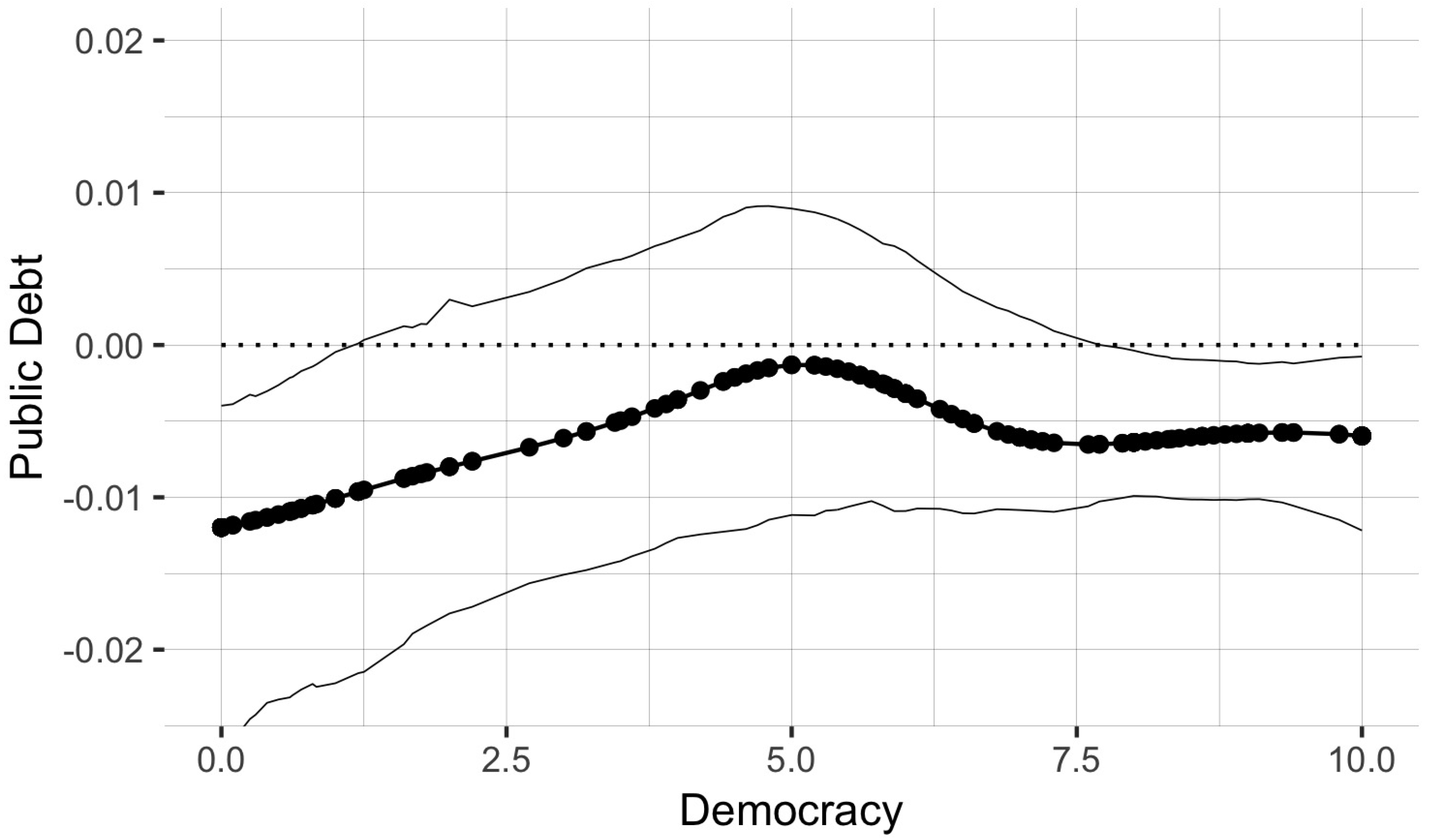
Figure 1 displays country-specific coefficient estimates for the public debt variable from the semi-parametric regression model in Table 1’s Column 10 along with 95% bootstrap percentile confidence intervals.5 We first observe that more public debt leads to lower economic growth for countries with democracy scores less than one and higher than 7.6, holding other factors fixed. This result is partially consistent with the existing literature that found an adverse effect of more public debt on growth for countries with weak institutional quality. However, we also found that countries with a high democracy score had a statistically-significant negative relationship between public debt and economic growth in the long run. We found that public debt had no significant effect on growth for the countries with a democracy score between one and 7.6. Notably, the impact of public debt on growth for countries with a median level of democracy score reduced to values around zero, which is therefore economically insignificant as well.

We find that the quartile values for the public debt coefficient estimates were −0.0093, −0.0071, and −0.0064, respectively, for the 25th, 50th, and 75th percentiles. Moreover, countries with zero democracy had the maximum value of estimates −0.012, whereas advanced countries with a democracy score of 10 had the median coefficient estimate. This result implies heterogeneity in the effect of debt on growth with different magnitudes for the two country groups. From another perspective, we found evidence of heterogeneity observing geographical differences within these two groups of countries. These results are particularly relevant to policy decisions suggesting fiscal policy sustainability for the low-income countries, as well as emerging and developed countries. However, we should note that debt sustainability is important for highly indebted Euro area countries such as Greece, Portugal, and Spain, but not the case for Japan.

We should emphasize that our results did not indicate any tipping point or threshold level for the debt-to-GDP ratio beyond which economic growth is adversely affected. For the two country groups separately, we observed debt-to-GDP ratios at different levels ranging from 16%–560% for the low democracy group and from 9%–196% for the high democracy group.

We did not find conclusive evidence in support of the direct effect of democracy on the coefficient of public debt as their effect appeared to be insignificant for all countries and economically insignificant for the advanced countries. In other words, if the democracy score of countries were to increase in the 10-year averages, it may not be indicative that these countries have an increasing or decreasing effect of public debt on growth in the long run.

4.2.1. Including the Period 2010–2014

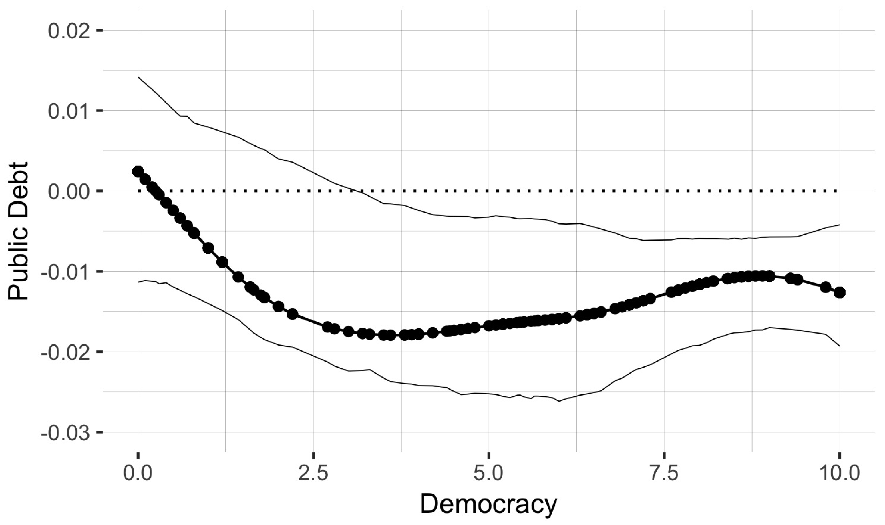
We further investigated the relationship between public debt and economic growth including the years from 2010–2014. Guyana, Nicaragua, Papua New Guinea, and Syria were not included in the extended dataset. Figure 2 displays functional coefficient estimates for the public debt variable using this dataset. In contrast to Figure 1, we found a statistically-significant negative effect of public debt on the growth for the countries with a democracy score higher than three. On average, public debt had a stronger effect on growth with an estimate of −0.0106 (1.5-fold increase) compared to the estimate from Column 9 in Table 1. We observed that countries with the highest democracy had a larger negative effect of public debt on growth at −0.013 than the effect obtained from the initial dataset. Moreover, the largest effect in magnitude was −0.018 for the countries having a democracy score of 3.5.6

Our results strongly suggest heterogeneity in the relationship between debt and growth as the countries in different geographical regions had statistically-significant estimates of different magnitudes. We also did not find any evidence on the direct effect of democracy on the public debt coefficient, which indicates the neutral effect of democracy on the public debt coefficient for all countries.

4.2.2. Policy Implications

We now turn to the contradictory result that we found in both Figure 1 and Figure 2 for the advanced countries. One may believe that good institutions, which we proxy by democracy in this paper, may help to alleviate the adverse effect of high public debt to ensure fiscal policy sustainability, to use government spending in productive sectors such as education and health, and to promote sustainable growth, among others. Japan is an example of this case having the largest debt-to-GDP ratio among advanced countries with strong economic indicators. The question may be then highly related to the quality of institutions of advanced countries. Relatedly, it has been widely discussed for the Euro area countries that the root of the public debt crisis in Europe is an excessive risk-taking behavior of economies due to over-borrowing (see Allen et al. (2015) and Yener et al. (2015)). In other words, countries within a widespread financial system rely heavily on external funds to finance their excess consumption, which eventually results in unsustainable public debt levels. To overcome this problem, governments adopt austerity fiscal policies with the risk of recession. Greece has been one of the examples of this situation.

The main reason behind our findings is that our democracy variables used in this paper captured only the political institutions of countries as explained in Section 3. However, it is widely argued that economic institutions, which are determined by the political process of a country, are one of the determinants of the prosperity of countries in the economic history (see Acemoglu and Robinson (2012) for further details). Therefore, our analysis requires additional variable such as the financial risk index, which can be a proxy for economic institutions and may have a variability within the advanced country group. We defer this analysis for future research.

In Section 5.1, we show the results from robustness checks conducted by excluding the most indebted advanced countries (i.e., Japan, Greece, Belgium, Ireland, Portugal, Italy, and Jamaica) to examine whether these countries may drive the main results for advanced countries. We found that the statistically-significant negative relationship between debt and growth for the advanced countries remained the same, which suggests that our core results for the highest democracy countries may be driven by country- and time-specific factors and spillover effects. Moreover, debt trajectory may have more explanatory power in the debt-growth nexus than the level of public debt (see Chudik et al. (2017) and Yener et al. (2017)). In fact, in our available dataset, we find all above-listed countries to have rising public debt levels regardless of their initial debt-to-GDP ratios. Lastly, we included Germany in the dataset to investigate whether our main results can be altered or not. With the inclusion of Germany in the analysis, our main results remained exactly the same.

4.2.3. Parameter Heterogeneity in the Relationship between Growth and Other Regressors

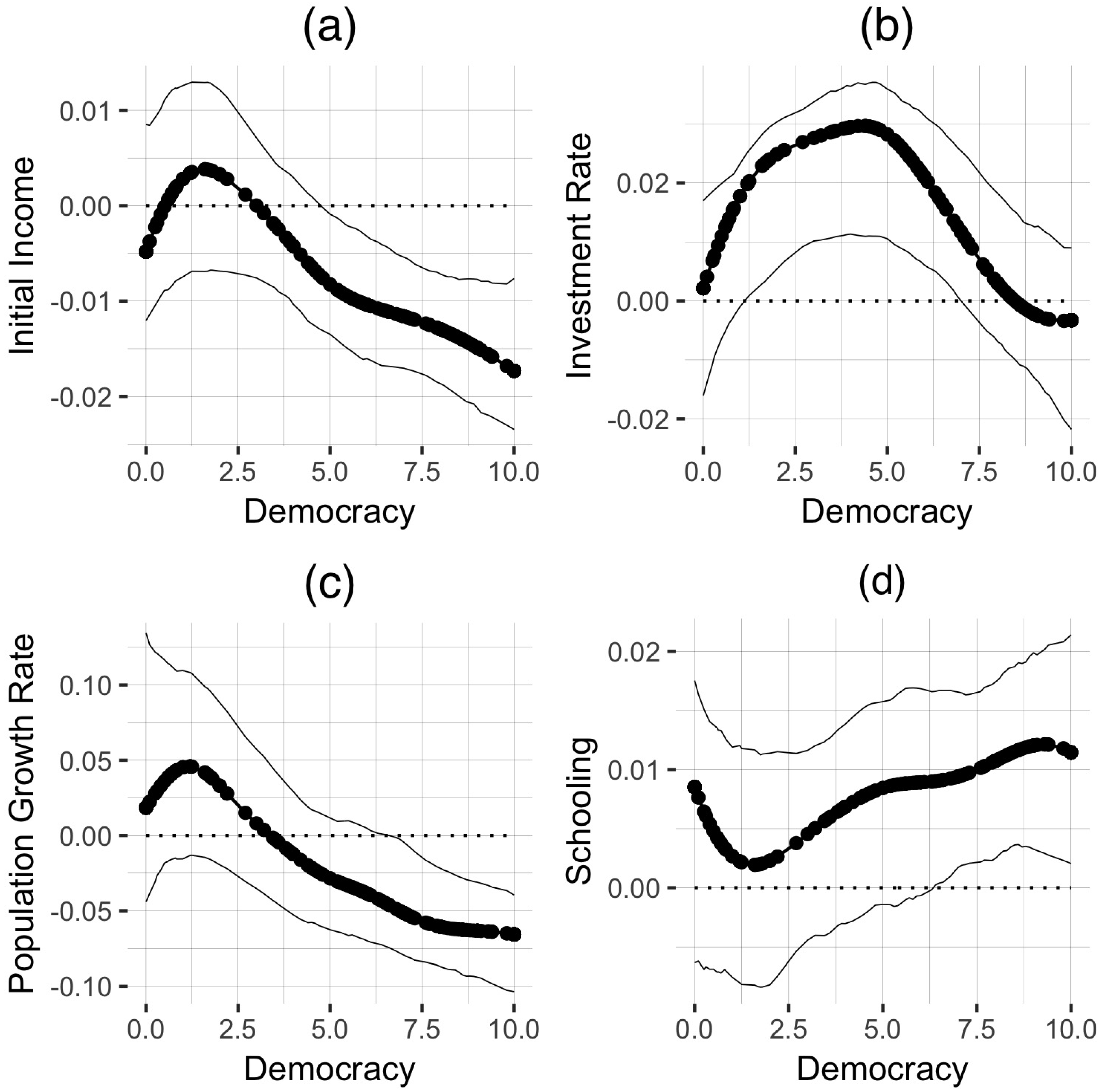
The curves in Figure 3 show how democracy affects the coefficients of other conditioning variables. Figure 3a shows that countries with an institutionalized democracy, a score higher than 4.7, had an increasing significant negative effect of initial income on economic growth, which confirms the conditional $\beta$-convergence hypothesis. The curve in Figure 3b exhibits a significant positive and an inverse U-shaped relationship between the real investment rate and the real GDP per capita growth rate for the countries with a democracy score between 1.2 and 7. Figure 3c indicates that a higher population growth rate was associated with a slowdown in economic growth for the countries with a democracy score greater than 6.6. Figure 3d shows that schooling had a significant positive effect on the growth rate for the countries with a democracy score greater than 6.3. For each regressor, except for the investment rate, there was a heterogeneous relationship in the effect of the variable on the economic growth rate for the mid- and high-level democracy score countries.

5. Robustness Checks

In this section, we describe how various robustness exercises used to examine whether our core results remain the same using additional model specifications.7

5.1. Influential Countries

Our primary investigation was undertaken to understand how sensitive the results are for advanced countries notated in Figure 1 and using respective datasets. In the dataset for the period 1980–2009, Japan, Jamaica, and Belgium are the countries with a democracy score of 10 having the highest public debt-to-GDP ratio. When we only exclude Japan, our core results in Figure 1 remain the same. When we exclude the three countries listed above, we lose the statistical significance of the estimates for countries with high democracy scores. In part, the insignificant coefficient estimates for advanced countries occurs because we lose nine data points in the neighborhood of each point estimation. We also ran our semi-parametric regression model with the initial dataset excluding Guyana, Nicaragua, Papua New Guinea, and Syria, as these countries are not available in the extended dataset. We find the same functional coefficient curve as in Figure 2 with fewer countries having statistically-significant coefficient estimates (i.e., countries with democracy scores higher than 6.8). For further investigation, we performed two additional econometric exercises by excluding Guyana only and testing Nicaragua, Papua New Guinea, and Syria together from the initial dataset. We found that the Guyana dataset might have driven our main finding for low democracy countries in Figure 1.

We performed the same econometric exercise for the extended dataset (i.e., for the years 1980–2014), excluding Japan, Greece, Belgium, Ireland, Portugal, Italy, and Jamaica. When we excluded Japan and Greece from the dataset, our core results in Figure 2 remained the same. When we excluded all seven countries listed above, our core results in Figure 2 remained the same with the same magnitude and functional coefficient curve. Thus, these results indicate that a high debt-to-GDP ratio may not be the main factor for the statistically-significant negative relationship between public debt and growth for the highest democracy countries. Specifically, in our study, being consistent with Kourtellos et al.’s (2013) findings, we find that low and high democracy countries have a negative effect of debt on growth regardless of their public debt-to-GDP ratio.

5.2. Alternative Measure for Democracy

We examined whether our main results were sensitive to different measures of institutional quality such as executive constraints obtained from the same data source, Polity IV. We found that countries with an executive constraint score less than 2.2 and higher than 5.8 had a statistically-significant negative relationship between public debt and growth for the period 1980–2009. This result does not alter the conclusions drawn from our main results; that is, institutional quality is an essential factor that governs the effect of public debt on growth.

We further tested our main results using Freedom House’s historical data on political rights and civil liberties. For the period 1980–2009, our findings indicated that countries with an index of political rights above 2.7 and below 4.5 (and with an index of civil liberties between 3.1 and 5.0) had a statistically-significant negative estimate of public debt on economic growth. For the period 1980–2014, we found a statistically-significant negative effect of public debt on growth for the countries whose political rights index was between 5.1 and 6.7 and whose civil liberty index was between 3.9 and 6.4. Overall, our core results were robust to different measures of democracy. However, we lost the statistical significance of a public debt coefficient estimate for the advanced countries.

5.3. Additional Control Variables

We estimated the semiparametric smooth coefficient model that includes such additional country characteristics as government spending, trade openness, fertility, and life expectancy. In separate econometric exercises for each additional control variable, we revealed similar results as shown in Figure 1 and Figure 2. Thus, the qualitative implications of our core results remained unchanged in the model.

6. Conclusions

In this study, we employed a semi-parametric smooth coefficient model with an endogenous variable in the nonparametric part to analyze the heterogeneous relationship between debt and growth with two different time frames. Our paper contributes to the literature by taking the institutional differences across countries into account in a flexible modelling approach and provides conclusive evidence of heterogeneity in the debt-growth relationship in the given sample.

Our results are consistent with the previous literature that identified an average negative and statistically-significant effect of public debt on growth. However, our semi-parametric model also identifies heterogeneity in the growth effect of public debt. Mainly, we find strong evidence that countries we studied with a democracy score less than one and higher than 7.6 have an adverse effect of debt on growth for the period 1980–2009. The magnitude of the effect of public debt on growth varies across countries with different institutional quality. Our findings for the period 1980–2014 also provide conclusive evidence in support of the negative and significant relationship between debt and growth for the countries with a democracy score higher than three. Our core results from Figure 1 suggest that a 10-percentage point increase in the debt-to-GDP ratio is associated with a 0.12% and 0.071% decrease in the subsequent 10-year period real GDP growth rate for the zero democracy countries and for the countries with a democracy score of 10, respectively. The public debt appears to have a more profound effect on growth for the advanced countries after the most recent years are considered. Specifically, the 10-year average real GDP growth rate decreased by 0.13% when the debt-to-GDP ratio surged by ten percentage points.

In future research, we will certainly incorporate more variables that are among the determinants of economic institutions of countries to better understand the effect of public debt on economic growth.

References

- Acemoglu, Daron, Simon Johnson, and James A. Robinson. 2001. The colonial origins of comparative development: An empirical investigation. American Economic Review 91: 1369–401. [Google Scholar] [CrossRef]
- Acemoglu, Daron, Simon Johnson, James A. Robinson, and Pierre Yared. 2005. From education to democracy? American Economic Review 95: 44–49. [Google Scholar] [CrossRef]
- Acemoglu, Daron, Suresh Naidu, Pascual Restrepo, and James A. Robinson. 2015. Democracy does cause growth. Journal of Political Economy. [Google Scholar] [CrossRef]
- Acemoglu, Daron, and James A. Robinson. 2012. Why Nations Fail: The Origins of Power, Prosperity, and Poverty. New York: Currency. [Google Scholar]
- Allen, Franklin, Elena Carletti, Itay Goldstein, and Agnese Leonello. 2015. Moral hazard and government guarantees in the banking industry. Journal of Financial Regulation 1: 1–21. [Google Scholar] [CrossRef]
- Azariadis, Costas, and Allan Drazen. 1990. Threshold externalities in economic development. The Quarterly Journal of Economics 105: 501–26. [Google Scholar] [CrossRef]
- Barro, Robert J., and Xavier I. Salai-Martin. 1995. Economic Growth. New York: McGraw-Hill. [Google Scholar]
- Baum, Anja, Cristina Checherita-Westphal, and Philipp Rother. 2013. Debt and growth: New evidence for the euro area. Journal of International Money and Finance 32: 809–21. [Google Scholar] [CrossRef]
- Bernal, Raquel, and Michael P. Keane. 2011. Child care choices and children’s cognitive achievement: the case of single mothers. Journal of Labor Economics 29: 459–12. [Google Scholar] [CrossRef]
- Bohn, Henning. 1995. The sustainability of budget deficits in a stochastic economy. Journal of Money, Credit and Banking 27: 257–71. [Google Scholar] [CrossRef]
- Cai, Zongwu, Mitali Das, Huaiyu Xiong, and Xizhi Wu. 2006. Functional coefficient instrumental variables models. Journal of Econometrics 133: 207–41. [Google Scholar] [CrossRef]
- Cai, Zongwu, and Qi Li. 2008. Nonparametric estimation of varying coefficient dynamic panel data models. Econometric Theory 24: 1321–42. [Google Scholar] [CrossRef]
- Caner, Mehmet, Thomas Grennes, and Fritzi Koehler-Geib. 2010. Finding the Tipping Point-When Sovereign Debt Turns Bad. Technical Report. Washington, DC: The World Bank. [Google Scholar]
- Cecchetti, Stephen G., Madhusudan S. Mohanty, and Fabrizio Zampolli. 2010. The Future of Public Debt: Prospects and Implications. Technical Report. Basel: Bank for International Settlements. [Google Scholar]
- Cecchetti, Stephen G., Madhusudan S. Mohanty, and Fabrizio Zampolli. 2011. The Real Effects of Debts. Technical Report. Basel: Bank for International Settlements. [Google Scholar]
- Checherita-Westphal, Cristina, and Philipp Rother. 2012. The impact of high government debt on economic growth and its channels: An empirical investigation for the euro area. European Economic Review 56: 1392–405. [Google Scholar] [CrossRef]
- Chen, Xiaohong. 2007. Large sample sieve estimation of semi-nonparametric models. In Handbook of Econometrics. Edited by James J. Heckman and Edward E. Leamer. New York: Springer, vol. 6B, pp. 5549–32. [Google Scholar]
- Chudik, Alexander, Kamiar Mohaddes, Hashem M. Pesaran, and Mehdi Raissi. 2017. Is there a debt-threshold effect on output growth? The Review of Economics and Statistics 99: 135–50. [Google Scholar] [CrossRef]
- Das, Mitali. 2005. Instrumental variables estimators for nonparametric models with discrete endogenous variables. Journal of Econometrics 124: 335–61. [Google Scholar] [CrossRef]
- Delgado, Michael S., Deniz Ozabaci, Yiguo Sun, and Subal C. Kumbhakar. 2015. Smooth Coefficient Models With Endogenous Environmental Variables. Technical Report. West Lafayette: Purdue University. [Google Scholar]
- Durlauf, Steven N., Andros Kourtellos, and Artur Minkin. 2001. The local solow growth model. European Economic Review 45: 928–40. [Google Scholar] [CrossRef]
- Eberhardt, Markus, and Andrea F. Presbitero. 2013. This Time They Are Different: Heterogeneity and Nonlinearity in The Relationship Between Debt and Growth. Technical Report. Washington, DC: IMF. [Google Scholar]
- Eberhardt, Markus, and Andrea F. Presbitero. 2015. Public debt and growth: heterogeneity and non-linearity. Journal of International Economics 97: 45–58. [Google Scholar] [CrossRef]
- Égert, Balázs. 2015. Public debt, economic growth and nonlinear effects: Myth or reality? Journal of Macroeconomics 43: 226–38. [Google Scholar] [CrossRef]
- Elmendorf, Douglas W., and N. Gregory Mankiw. 1999. Government debt. In Handbook of Macroeconomics. Edited by John B. Taylor. Oxford: Taylor and Michael Woodford. [Google Scholar]
- Glaeser, Edward L., Rafael La Porta, Florencio Lopez-De-Silanes, and Andrei Shleifer. 2004. Do institutions cause growth? Journal of Economic Growth 9: 271–303. [Google Scholar] [CrossRef]
- Gonzáles, Andrés, Timo Teräsvirta, and Dick VanDijk. 2005. Panel Smooth Transition Regression Models. Technical Report. Stockholm: Stockholm School of Economics. [Google Scholar]
- Härdle, Wolfgang, and Steve J. Marron. 1991. Bootstrap simultaneous error bars for nonparametric regression. The Annals of Statistics 19: 778–96. [Google Scholar] [CrossRef]
- Henderson, Daniel J., Subal C. Kumbhakar, and Christopher F. Parmeter. 2012. A simple method to visualize results in nonlinear regression models. Economics Letters 117: 578–81. [Google Scholar] [CrossRef]
- Henderson, Daniel J., Chris Papageorgiou, and Christopher F. Parmeter. 2011. Growth empirics without parameters. The Economic Journal 122: 125–54. [Google Scholar] [CrossRef]
- Henderson, Daniel J., and Christopher F. Parmeter. 2015. Applied Nonparametric Econometrics. New York: Cambridge University Press. [Google Scholar]
- Jalles, Joao T. 2011. The impact of democracy and corruption on the debt-growth relationship in developing countries. Journal of Economic Development 36: 41–72. [Google Scholar]
- Ketteni, Elena, Theofanis P. Mamuneas, and Thanasis Stengos. 2007. Nonlinearities in economic growth: A semiparametric approach applied to information technology data. Journal of Macroeconomics 29: 555–68. [Google Scholar] [CrossRef]
- Kourtellos, Andros. 2011. Modeling parameter heterogeneity in cross-country regression models. In Economic Growth and Development (Frontiers of Economics and Globalization). Edited by O. de La Grandville. Bingley: Emerald Group Publishing Limited, pp. 579–604. [Google Scholar]
- Kourtellos, Andros, Thanasis Stengos, and Chih Ming Tan. 2013. The effect of public debt on growth in multiple regimes. Journal of Macroeconomics 38: 35–43. [Google Scholar] [CrossRef]
- Kourtellos, Andros, Thanasis Stengos, and Chih Ming Tan. 2016. Structural thresold regression. Econometric Theory 32: 827–60. [Google Scholar] [CrossRef]
- Kumbhakar, Subal C., and Kai Sun. 2012. Estimation of tfp growth: A semiparametric smooth coefficient approach. Empirical Economics 43: 1–24. [Google Scholar] [CrossRef]
- Li, Qi, Cliff J. Huang, Dong Li, and Tsu-Tan Fu. 2002. Semiparametric smooth coefficient models. Journal of Business and Economic Statistics 20: 412–22. [Google Scholar] [CrossRef]
- Liu, Zhenjuan, and Thanasis Stengos. 1999. Non-linearities in cross-country growth regressions: A semiparametric approach. Journal of Applied Econometrics 14: 527–38. [Google Scholar] [CrossRef]
- Mamuneas, Theofanis P., Andreas Savvides, and Thanasis Stengos. 2006. Economic development and the return to human capital: A smooth coefficient semiparametric approach. Journal of Applied Econometrics 21: 111–32. [Google Scholar] [CrossRef]
- Marshall, Monty G., Ted R. Gurr, and Keith Jaggers. 2016. Polity Iv Project: Dataset Users’ Manual. Technical Report. Vienna: Center for Systemic Peace. [Google Scholar]
- Minea, Alexandru, and Antoine Parent. 2012. Is High Public Debt Always Harmful to Economic Growth? Reinhart And Rogoff and Some Complex Nonlinearities. Technical Report. Clermont-Ferrand: Centre d’Études et de Recherches sur le Développement International. [Google Scholar]
- Minier, Jenny A. 2007. Institutions and parameter heterogeneity. Journal of Macroeconomics 29: 595–611. [Google Scholar] [CrossRef]
- Newey, Whitney K., and James L. Powell. 2003. Instrumental variable estimation of nonparametric models. Econometrica 71: 1565–78. [Google Scholar] [CrossRef]
- Newey, Whitney K., James L. Powell, and Francis Vella. 1999. Nonparametric estimation of triangular simultaneous equations models. Econometrica 67: 565–603. [Google Scholar] [CrossRef]
- Ozabaci, Deniz, Daniel J. Henderson, and Liangjun Su. 2014. Additive nonparametric regression in the presence of endogenous regressors. Journal of Business & Economic Statistics 32: 555–75. [Google Scholar]
- Panizza, Ugo, and Andrea F. Presbitero. 2014. Public debt and economic growth: is there a causal effect. Journal of Macroeconomics 41: 21–41. [Google Scholar] [CrossRef]
- Racine, Jeffrey S., and Qi Li. 2004. Nonparametric estimation of regression functions with both categorical and continuous data. Journal of Econometrics 119: 99–130. [Google Scholar] [CrossRef] [Green Version]
- Reinhart, Carmen M., Vincent R. Reinhart, and Kenneth S. Rogoff. 2012. Public debt overhangs: advanced-economy episodes since 1800. Journal of Economic Perspectives 26: 69–86. [Google Scholar] [CrossRef]
- Reinhart, Carmen M., and Kenneth S. Rogoff. 2010. Growth in a Time of Debt. NBER Working Paper No. 15639. Cambridge, MA, USA: NBER. [Google Scholar]
- Temple, Jonathan. 1999. The new growth evidence. Journal of Economic Literature 37: 112–56. [Google Scholar] [CrossRef]
- Vaona, Andrea, and Stefano Schiavo. 2007. Nonparametric and semiparametric evidence on the long-run effects of inflation on growth. Economics Letters 94: 452–58. [Google Scholar] [CrossRef]
- Woo, Jaejoon, and Manmohan S. Kumar. 2015. Public debt and growth. Economica 82: 705–39. [Google Scholar] [CrossRef]
- Wright, Alan, and Kari Grenade. 2014. Determining optimal public debt and debt-growth dynamics in the caribbean. Research in Applied Economics 6: 87–115. [Google Scholar] [CrossRef]
- Yener, Haluk, Thanasis Stengos, and Ege M. Yazgan. 2015. Survival Maximizing Leverage of an Economy: The Case of Greece. Technical Report, Discussion Paper. Guelph: University of Guelph. [Google Scholar]
- Yener, Haluk, Thanasis Stengos, and Ege M. Yazgan. 2017. Analysis of the seeds of the debt crisis in europe. The European Journal of Finance 23: 1589–610. [Google Scholar] [CrossRef]