Article

Multivariate Student versus Multivariate Gaussian Regression Models with Application to Finance

by
Thi Huong An Nguyen
1,2,†,
Anne Ruiz-Gazen
1,*,†,
Christine Thomas-Agnan
1,† and
Thibault Laurent
3,†
1
Toulouse School of Economics, University of Toulouse Capitole, 21 allée de Brienne, 31000 Toulouse, France
2
Department of Economics, DaNang Architecture University, Da Nang 550000, Vietnam
3
Toulouse School of Economics, CNRS, University of Toulouse Capitole, 31000 Toulouse, France
*
Author to whom correspondence should be addressed.
These authors contributed equally to this work.
J. Risk Financial Manag. 2019, 12(1), 28; https://doi.org/10.3390/jrfm12010028
Submission received: 29 December 2018 / Revised: 24 January 2019 / Accepted: 31 January 2019 / Published: 9 February 2019
(This article belongs to the Special Issue Applied Econometrics)

Abstract

:
To model multivariate, possibly heavy-tailed data, we compare the multivariate normal model (N) with two versions of the multivariate Student model: the independent multivariate Student (IT) and the uncorrelated multivariate Student (UT). After recalling some facts about these distributions and models, known but scattered in the literature, we prove that the maximum likelihood estimator of the covariance matrix in the UT model is asymptotically biased and propose an unbiased version. We provide implementation details for an iterative reweighted algorithm to compute the maximum likelihood estimators of the parameters of the IT model. We present a simulation study to compare the bias and root mean squared error of the ensuing estimators of the regression coefficients and covariance matrix under several scenarios of the potential data-generating process, misspecified or not. We propose a graphical tool and a test based on the Mahalanobis distance to guide the choice between the competing models. We also present an application to model vectors of financial assets returns.

1. Introduction

Many applications involving models for multivariate data underline the limitations of the classical multivariate Gaussian model, mainly due to its inability to model heavy tails. It is then natural to turn attention to a more flexible family of distributions, for example the multivariate Student distribution.
In one dimension, the generalized Student distribution encompasses the Gaussian distribution as a limit when the number of degrees of freedom or shape parameter tends to infinity, allowing for heavier tails when the shape parameter is small. As we will see, a first difficulty in higher dimensions is that there are several kinds of multivariate Student distributions; see for example Johnson and Kotz (1972) and more recently Kotz and Nadarajah (2004). A nice summary of the properties of the multivariate Student distribution that we will use later on in this paper, and its comparison with the Gaussian multivariate, can be found in Roth (2013).
Before going further, let us mention that it is not so easy to have a clear overview of the results in terms of Student regression models for at least three reasons. The first reason is that this topic is scattered, with some papers in the statistical literature and others in the econometrics literature, sometimes without cross-referencing. The second reason is that the word “multivariate” is sometimes misleading since, as we will see, the multivariate Student is used to define a univariate regression model. At last, the distinction between models UT and IT (see below) is not always clearly announced in the papers. Other miscellaneous reasons are that some authors just fit the distribution without covariates and finally that some authors consider the degrees of freedom as fixed, whereas others estimate it. Our first purpose here is to lead the reader through this literature and gather the results concerning the maximum likelihood estimators of the parameters in the multivariate UT and IT models with a common notation. In the present paper, we consider a multivariate dependent vector and a linear regression model with different assumptions on the error term distribution. The most common and convenient assumption is the Gaussian distribution. For a Gaussian vector, the assumption of independent coordinates is equivalent to the assumption of uncorrelated coordinates. Such an equivalence is no longer true when considering a multivariate Student distribution. We thus consider two cases: uncorrelated (UT) on the one hand and independent Student (IT) error vectors on the other hand.
The purpose of this paper is to contribute to the UT and IT models as well as to their comparisons. First of all, for the UT model, we extend to the multivariate case the results of Zellner (1976) for the derivation of the maximum likelihood estimators and Zellner’s formula (Zellner (1976)) for the bias of the covariance matrix estimator, and we prove that it does not vanish asymptotically. For the multivariate IT model, in the same spirit as Lange and Sinsheimer (1993), we provide details for the implementation of an iterative reweighted algorithm to compute the maximum likelihood estimators of the parameters. We devise a simulation study to measure the impact of misspecification on the bias, variance, and mean squared error of these different parameters’ estimates under several data-generating processes (Gaussian, UT, and IT) and try to answer the question: what are the consequences of a wrong specification? Finally we introduce a new procedure for model selection based on the knowledge of the distribution of the Mahalanobis distances under the different data-generating processes (DGP).
One application attracted our attention in the finance literature. The work in Platen and Rendek (2008) identified the Student distribution with between three and five degrees of freedom, with a concentration around four, as the typical distribution for modeling the distribution of log-returns of world stock indices. They embedded the Student t in the class of generalized hyperbolic distributions, itself a subclass of the normal/independent family. For bivariate returns, the work in Fung and Seneta (2010) compared a multivariate Student IT model with an alternative model obtained by a more complex mixing representation from the point of view of asymptotic tail dependence. The work in Hu and Kercheval (2009) insisted on the fact that the choice of distribution matters when optimizing the portfolio. They found that the Student UT model performs the best in the class of symmetric generalized hyperbolic distributions. The work in Kan and Zhou (2017) advocated using a multivariate IT model for fitting the joint distribution of stock returns for a few fixed values of the degrees of freedom parameter and showed that this model outperforms the multivariate Gaussian.
In Section 2, after recalling the univariate results, we extend the results of Zellner (1976) for the derivation of the maximum likelihood estimators and its properties in the UT model and propose an iterative implementation for the IT model. We present the results of the simulation study in Section 3 and of the model selection strategy in Section 4 using a toy example and a dataset from finance. Section 5 summarizes the findings and gives recommendations.

2. Multivariate Regression Models

2.1. Literature Review

In order to define a Student regression model, even in the univariate case (single dependent variable), one needs to use the multivariate Student distribution to describe the joint distribution of the vector of observations for the set of statistical units. There are mainly two options, which were described in Kelejian and Prucha (1985) for the case of univariate regression. Indeed, the property of the equivalence between the independence and uncorrelatedness for components of a Gaussian vector are not satisfied anymore for a multivariate Student vector. One option, which we will call the IT model (for independent t-distribution) in the sequel, considers that the components of the random disturbance vector of the regression model are independent with the same marginal Student distribution. The second option, which we will call the UT model (for uncorrelated t-distribution), postulates a joint multivariate Student distribution for the vector of disturbances. Note that in both models, the marginal distribution of each component still is Student univariate.
The work in Zellner (1976) introduced a univariate Student regression model of the type UT with known degrees of freedom and studied the corresponding maximum likelihood and Bayesian estimators (with some adapted priors). The work in Singh (1988) considered the case of univariate Student regression with the UT model and with unknown degrees of freedom and derived an estimator of the degrees of freedom and subsequent estimators of the other parameters. However, Fernandez and Steel (1999) showed that this estimator was not consistent. Using one possible representation of the multivariate Student distribution, Lange and Sinsheimer (1993) embedded univariate Student regression with the UT model in a larger family of regression models (with normal/independent error distributions) and developed EM algorithms to compute their maximum likelihood estimates, as in Dempster et al. (1978).
In the framework of the spherical error distribution, which includes the Student error model as a special case, the work in Fraser and Ng Kai (1980) proved an extension to the multivariate case of Zellner’s result stating that inference about the parameters corresponds closely to that under normal theory. Motivated by a financial application, the work in Sutradhar and Ali (1986) used a multivariate UT Student regression model with moment estimators instead of maximum likelihood and allowing the degrees of freedom to be unknown.
The univariate IT model was introduced in Fraser (1979) and compared to the UT model in Kelejian and Prucha (1985).
Concerning multivariate IT Student distributions, there was first a collection of results or applications for the case without regressors. The work in McNeil et al. (2005) used a representation of the multivariate IT Student distribution to derive an algorithm of the EM type for computing the maximum likelihood parameter estimators. They used the framework of normal mixture distributions in which the Student distribution can be expressed as a combination of a Gaussian random variable and an inverse gamma random variable. More recently, the work in Dogru et al. (2018) proposed a more robust extension, replacing maximum likelihood by a kind of M-estimation method based on the minimization of a q-entropy criterion. For the multivariate Student IT model, the work in Prucha and Kelejian (1984) derived the normal equations for the maximum likelihood estimators and their asymptotic properties with known degrees of freedom in a framework that encompasses our multivariate Student regression case. The work in Lange et al. (1989) illustrated this multivariate IT model on several examples. The work in Lange and Sinsheimer (1993) considered the framework of normal/independent error distributions (same as normal variance mixtures) and derived the EM algorithm for the maximum likelihood estimators in a model with covariates. The works in Liu and Rubin (1995) and Liu (1997) developed extensions of the EM algorithm for the multivariate IT model with known or unknown degrees of freedom, with or without covariates and with or without missing data. The work in Katz and King (1999) fit a multivariate IT distribution to multiparty electoral data. The work in Fernandez and Steel (1999) attracted attention to the fact that maximum likelihood inference can encounter problems of unbounded likelihood when the number of degrees of freedom is considered unknown and has to be estimated. Before engaging in the use of the multivariate Student distribution, it is wise to read Hofert (2003), which explained some traps to be avoided. One difficulty indeed is to be aware that some authors parametrize the multivariate Student distribution using the covariance matrix, while others use the scatter matrix, sometimes with the same notation for either one.
We consider the following version of the Student p-multivariate distribution denoted by T p ( μ , Σ , ν ) with μ being the p-vector of means, Σ being the p × p covariance matrix, and ν > 2 the degrees of freedom. It is defined, for a p-vector z , by the probability density function:
p ( z | μ , Σ , ν ) = f ( ν ) det ( Σ ) 1 / 2 1 + 1 ν 2 ( z μ ) T Σ 1 ( z μ ) ( ν + p ) / 2 ,
where T denotes the transpose operator, f ( ν ) = Γ [ ( ν + p ) / 2 ] Γ ( ν / 2 ) ( ν 2 ) p / 2 π p / 2 and Γ is the usual Gamma function.
Note that the assumption ν > 2 implies the existence of the first two moments of the distribution and that the above density function is parametrized in terms of the covariance matrix. In most of the literature on multivariate Student distributions, the density is rather parametrized as a function of the scatter matrix ( ( ν 2 ) / ν ) Σ . Using the covariance matrix parametrization facilitates the comparison with the Gaussian distribution. We first recall some results in the univariate regression context.

2.2. Univariate Regression Case Reminder

In the univariate regression case and for a sample of size n, we have a one-dimensional dependent variable Y i , i = 1 , , n , whose values are stacked in a vector Y , and K explanatory variables defining a n × ( K + 1 ) design matrix X including the constant.
The regression model is written as Y = X β + ϵ , where β = ( β 0 , , β K ) T is a ( K + 1 ) -dimensional vector of parameters and the error term ϵ = ( ϵ 1 , , ϵ n ) T is an n-dimensional vector. If we consider that the design matrix is fixed with rank K + 1 or look at the distribution of ϵ conditional on X , the usual assumptions are the following. The errors ϵ i , i = 1 , , n , are independent and identically distributed (i.i.d.) with expectation zero and equal variance σ 2 . In this context, it is well known that the least squares estimator of β is equal to:
β ^ = ( X T X ) 1 X T Y
while the classical σ 2 estimator is σ ^ 2 = ϵ ^ T ϵ ^ / ( n K 1 ) where ϵ ^ = Y X β ^ . These estimators are unbiased. In the case of a Gaussian error distribution, the estimator β ^ coincides with the maximum likelihood estimator of β , while the maximum likelihood estimator of σ 2 is equal to σ ^ 2 multiplied by ( n K 1 ) / n and is only asymptotically unbiased. In the Gaussian case, there is an equivalence between the ϵ i being independent or uncorrelated. However, this property is no longer true for a Student distribution. This means that one should distinguish the case of uncorrelated errors from the case of independent errors. The case where the errors ϵ i , i = 1 , , n , follow a joint n-dimensional Student distribution with diagonal covariance matrix and equal variance is called the UT model, and its coordinates are uncorrelated, but not independent. Interestingly, the maximum likelihood method for the UT model with known degrees of freedom leads to the least squares estimator (2) of β (Zellner (1976)). This property is true for more general distributions as long as the likelihood is a decreasing function of ϵ T ϵ . Concerning the error variance, the maximum likelihood estimator is ( n K 1 ) ν σ ^ 2 / ( n ( ν 2 ) ) and is biased even asymptotically Zellner (1976). For the independent case, we assume that the errors ϵ i , i = 1 , , n , are i.i.d. with a Student univariate distribution and known degrees of freedom. The maximum likelihood estimators belong to the class of M-estimators, which are studied in detail in Chapter 7 of Huber and Ronchetti (2009). These estimators are defined through implicit equations and can be computed using an iterative reweighted algorithm.
In what follows, we consider the case of a multivariate dependent variable and propose to gather and complete the results from the literature. As we will see, the results derived in the multivariate case are very similar to their univariate counterpart. In particular, the maximum likelihood estimator of the error covariance matrix is biased for the uncorrelated Student model, while there is a need to define an iterative algorithm for the independent Student model.

2.3. The Multivariate Regression Model

Let us consider a sample of size n, and for i = 1 , , n , let us denote the L-dimensional dependent vector by:
Y i = ( y i 1 , , y i L ) T .
For K explanatory variables, the design matrix is of size L × ( K + 1 ) L and is given by:
X i = I L x i T
for i = 1 , , n , with the ( K + 1 ) -vector x i = ( 1 , x i 1 , , x i K ) T , I L the identity matrix with dimension L, and ⊗ the usual Kronecker product. The parameter of interest is a ( K + 1 ) L vector given by:
β = ( β 1 T , , β L T ) T ,
where β j = ( β 0 j , , β K j ) T , for j = 1 , , L , and the L-vector of errors is denoted by:
ϵ i = ( ϵ i 1 , , ϵ i L ) T
for i = 1 , , n . We consider the linear model:
Y i = X i β + ϵ i
with E ( ϵ i ) = 0 and i = 1 , , n . Using matrix notations, we can write Model (3) as:
Y = X β + ϵ
with the n L -vectors:
Y = ( Y 1 T , , Y n T ) T ,
ϵ = ( ϵ 1 T , , ϵ n T ) T
and the n L × ( K + 1 ) L matrix:
X = ( X 1 T , , X n T ) T .
In what follows, we make different assumptions on the distribution of ϵ and recall (for Gaussian and IT) or derive (for UT) the maximum likelihood estimators of the parameter β and of the covariance matrix of ϵ .

2.4. Multivariate Normal Error Vector

Let us first consider Model (4) with independent and identically distributed error vectors ϵ i , i = 1 , , n , following a multivariate normal distribution N L ( 0 , Σ ) with an L-vector of means equal to zero and an L × L covariance matrix Σ . This model is denoted by N, and the subscript N is used to denote the error terms ϵ N i , i = 1 , , n , and the parameters β N and Σ N of the model. The maximum likelihood estimators of β N and Σ N are:
β ^ N = ( X T X ) 1 X T Y ,
Σ ^ N = i = 1 n ϵ ^ N i ϵ ^ N i T n ,
where ϵ ^ N i = Y i X i β ^ N (see, e.g., Theorem 8.4 from Seber (2008)).
The estimator β ^ N is an unbiased estimator of β N while the bias of Σ ^ N is equal to ( ( K + 1 ) / n ) Σ N and tends to zero when n tends to infinity (see, e.g., Theorems 8.1 and 8.2 from Seber (2008)).
For data such as financial data, it is well known that the Gaussian distribution does not fit the error term well. Student distributions are known to be more appropriate because they have heavier tails than the Gaussian. As for the univariate case, for Student distributions, the independence of coordinates is not equivalent to their uncorrelatedness, and we consider below two types of Student distributions for the error term. In Section 2.5, the error vector ϵ is assumed to follow a Student distribution with n L dimensions and a particular block diagonal covariance matrix. More precisely, we assume that the error vectors ϵ i , i = 1 , , n , are identically distributed and uncorrelated but are not independent. In Section 2.6, however, we consider independent and identically distributed error vectors ϵ i , i = 1 , , n , with an L-dimensional Student distribution.

2.5. Uncorrelated Multivariate Student (UT) Error Vector

Let us consider Model (4) with uncorrelated and identically distributed error vectors ϵ i , i = 1 , , n , such that the vector ϵ follows a multivariate Student distribution T n L ( 0 , Ω , ν ) with known degrees of freedom ν > 2 and covariance matrix Ω = I n Σ . The L × L matrix Σ is the common covariance matrix of the ϵ i , i = 1 , , n . This model is denoted by UT, and the subscript U T is used to denote the error terms ϵ U T i , i = 1 , , n , and the parameters β U T , Ω U T , and Σ U T of the model. This model generalizes the model proposed by Zellner (1976) to the case of multivariate ϵ i s. We derive the maximum likelihood estimators of β U T and Σ U T in Proposition 1 and give the bias of the covariance estimator in Proposition 2. The proofs of the propositions are given in the Appendix A.
Proposition 1.
The maximum likelihood estimators of β U T and Σ U T are given by:
β ^ U T = X T X 1 X T Y , Σ ^ U T = ν ν 2 i = 1 n ϵ ^ U T i ϵ ^ U T i T n ,
where ϵ ^ U T i = Y i X i β ^ U T .
The next proposition gives the bias of the maximum likelihood estimators and generalizes Zellner’s result (Zellner (1976), p. 402) to the multivariate UT model. The maximum likelihood estimator of β U T coincides with the least squares and with the method of moment estimators and is unbiased. This is no longer the case for the maximum likelihood estimator of Σ U T , which is biased even asymptotically. This gives an example of a maximum likelihood estimator that is not asymptotically unbiased in a context where the random variables are not independent. It illustrates that the independence assumption is crucial to derive the usual properties of the maximum likelihood estimators. Note that the method of moments estimator is a consistent estimator of Σ U T (see Sutradhar and Ali (1986)).
Proposition 2.
The estimator β ^ U T is unbiased for β U T . The estimator Σ ^ U T is biased for Σ U T even asymptotically. More precisely,
E ( Σ ^ U T ) = n K n ν ν 2 Σ U T
A consequence of Proposition 2 is that an asymptotically unbiased estimator of Σ U T is given by Σ ˜ U T = i = 1 n ϵ ^ U T i ϵ ^ U T i T / n .

2.6. Independent Multivariate Student Error Vector
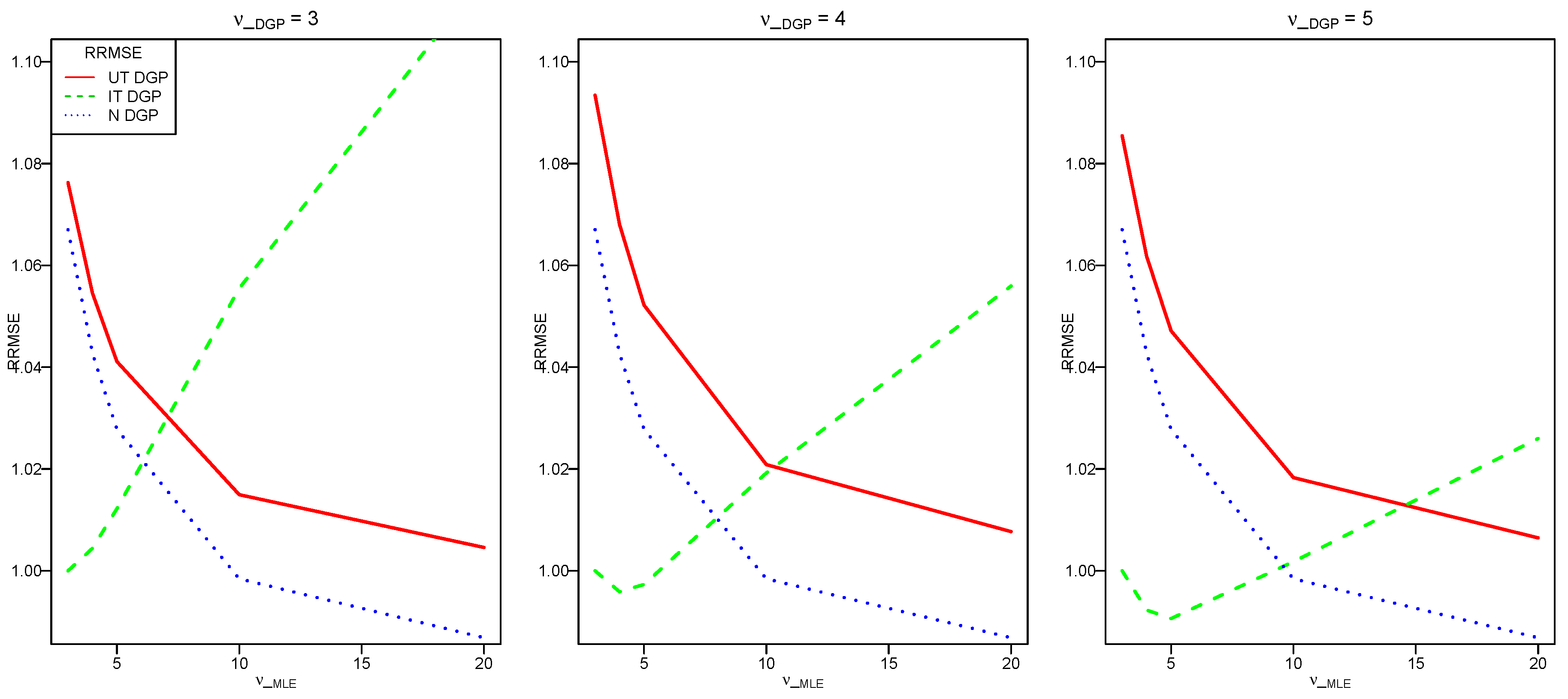
Let us consider Model (4) using the notations of Section 2.3 with i.i.d. ϵ i , i = 1 , , n , following a Student distribution with L dimensions and known degrees of freedom ν > 2 . We denote this model by IT and the parameters of the model by β I T and Σ I T . The IT model is a particular case of Prucha and Kelejian (1984) where the B matrix in Expression (2.1) in Prucha and Kelejian (1984) is equal to zero.
Following Prucha and Kelejian (1984), we derive the maximum likelihood estimators for the IT model.
Proposition 3.
The maximum likelihood estimators of β I T and Σ I T in the IT regression model satisfy the following implicit equations:
β ^ I T = i = 1 n w ^ I T i X i T Σ ^ I T 1 X i 1 i = 1 n w ^ I T i X i T Σ ^ I T 1 Y i Σ ^ I T = 1 n i = 1 n w ^ I T i ϵ ^ I T i ϵ ^ I T i T
w i t h : ϵ ^ I T i = Y i X i β ^ I T a n d w ^ I T i = ν + L ν 2 + ϵ ^ I T i T Σ ^ I T 1 ϵ ^ I T i .
These estimators are consistent estimators of β I T and Σ I T (see Theorem 3.2 in Prucha and Kelejian (1984)). In order to compute them, we propose to implement the following iterative reweighted algorithm in the same spirit as in Huber and Ronchetti (2009) for the univariate case (see also Lange et al. (1989)).
Step 0: Let:
β ^ I T ( 0 ) = ( X T X ) 1 X T Y ϵ ^ I T ( 0 ) = Y X β ^ I T ( 0 ) Σ ^ I T ( 0 ) = 1 n i = 1 n ϵ ^ I T i ( 0 ) ϵ ^ I T i ( 0 ) T
Step k→ Step ( k + 1 ), k > 0 :
w ^ I T i ( k + 1 ) = ν + L ν 2 + ϵ ^ I T i ( k ) Σ ^ I T ( k ) 1 ϵ ^ I T i ( k ) β ^ I T ( k + 1 ) = i = 1 n w ^ I T i ( k + 1 ) X i T Σ ^ I T ( k ) 1 X i 1 i = 1 n w ^ I T i ( k + 1 ) X i T Σ ^ I T ( k ) 1 Y i ϵ ^ I T ( k + 1 ) = Y X β ^ I T ( k + 1 ) Σ ^ I T ( k + 1 ) = 1 n i = 1 n w ^ I T i ( k + 1 ) ϵ ^ I T i ( k + 1 ) ϵ ^ I T i ( k + 1 ) T
The process is iterated until convergence. Note that this algorithm is given in detail in Section 7.8 of Huber and Ronchetti (2009) for a general class of univariate regression M-estimators. It is also sometimes called IRLS for iteratively-reweighted least squares and can be seen as a particular case of the EM algorithm (Dempster et al. (1978)).
Table 1 gathers the likelihoods and thus summarizes the three models of interest.

3. Simulation Study

3.1. Design

This study aims at comparing the properties of the estimators of β and Σ as defined in the previous section for the multivariate Gaussian (N), the uncorrelated multivariate Student (UT), and the independent multivariate Student (IT) error distributions, under several scenarios for the DGP. Note that for the UT model, we used the asymptotically unbiased estimator Σ ˜ U T to estimate Σ U T . We considered a variety of degrees of freedom ν D G P for the Student IT and UT models with a focus on values between three and five. We used the function rmvt from the R package mvnfast to simulate the Student distributions. For a sample size n = 1000 and a number of replications N = 10,000, we simulated an explanatory variable X following a Gaussian distribution N ( 45 , 10 ) . The parameter vector β and the covariance matrix Σ are respectively chosen to be:
β = β 01 β 11 β 02 β 12 = 2 3 4 3 ; Σ = σ 1 2 ρ σ 1 σ 2 ρ σ 1 σ 2 σ 2 2 = 2 0.5 0.5 1 .
Note that similar results are obtained with other choices of parameters.
For each DGP, we calculate a number of Monte Carlo performance measures of the estimators proposed in Section 2. The performances are measured by the Monte Carlo relative bias (RB) and the mean squared error (MSE), which are defined for an estimator θ ^ of a parameter θ by:
Bias ( θ ^ ) = 1 N i = 1 n θ ^ ( i ) θ RB ( θ ^ ) = 100 Bias ( θ ^ ) θ MSE ( θ ^ ) = 1 N i = 1 N θ ^ ( i ) θ 2 .
We also compute a relative root mean squared error (RRMSE) with respect to a baseline estimator θ ˜ as:
RRMSE ( θ ^ ) = MSE ( θ ^ ) MSE ( θ ˜ ) 1 / 2 .
In our case, the baseline estimator is the maximum likelihood estimator (MLE) corresponding to the DGP. For example, in Table 2, the RRMSE of the β ^ I T for the Gaussian DGP is the ratio of the MSE of β ^ I T with the degrees of freedom ν M L E and the MSE of β ^ N . Note that if θ ^ = θ ˜ , then the RRMSE of θ ^ is equal to one.

3.2. Estimators of the β Parameters

Table 3 reports the bias and the MSE of the Gaussian MLE estimator β ^ N , the UT MLE estimator β ^ U T ( ν DGP = 3 ), and the IT MLE estimator β ^ I T ( ν DGP = 3 ) when the model is well specified, i.e., under the corresponding DGP. The bias and MSE of the estimators of β are small and comparable under the Gaussian and the UT DGP, but smaller for the IT DGP. Note that, in our implementation, the results of the algorithm for the IT estimators are very similar to those obtained using the function heavyLm from the R package heavy.
In Table 2, we start considering misspecifications and report the corresponding relative values RB and RRMSE of the same estimators and the same DGP as in Table 3 with all possible combinations of DGP and estimation methods. The results indicate that the RB of β ^ are all very small. If the DGP is Gaussian and the estimator is IT, the RRMSE of coordinates of β ^ is about 1.09 . However, if the DGP is IT and the estimator is Gaussian, the RRMSE of coordinates of β ^ is higher (from 1.46–1.48). Hence for the Gaussian DGP, we do not loose too much efficiency using the IT estimator β ^ I T with three degrees of freedom. Inversely, we loose much more efficiency when using β ^ N for the IT DGP with three degrees of freedom.
In order to consider more degrees of freedom (3, 4, and 5), we now drop the bias and focus on the RRMSE. Table 4 indicates that the RRMSE of β ^ is very similar and close to one, with a maximum of 1.09 , except for the case of the N estimator under the IT DGP, where it can reach 1.48 . The work in Maronna (1976) provided theoretical asymptotic efficiencies of the Student versus the Gaussian estimators, the ratio of asymptotic variances being equal to ( ν 2 ) ( ν + L + 2 ) ν ( ν + L ) . The values obtained in Table 2 are very similar to these asymptotic values.
Figure 1 shows the performances in terms of RRMSE of the IT estimators β ^ 12 I T under different DGP as a function of the degrees of freedom of the IT estimator ( ν MLE ). The considered DGP are the Gaussian, UT, and IT DGP with the degrees of freedom ν DGP = 3 (respectively, ν DGP = 4 , ν DGP = 5 ) on the left (respectively, middle, right) plot. Overall, the RRMSE of β ^ 12 I T for the IT DGP has a down trend and then an up trend, while for the Gaussian and the UT DGP, the RRMSE are decreasing when ν MLE increases. The maximum RRMSE of β ^ 12 I T is around 1.09 under the UT DGP and is around 1.08 under the Gaussian DGP. It decreases then to one when ν MLE increases to twenty under the Gaussian and the UT DGP; thus, the risk under misspecification is not very high. The curve is U-shaped under the IT DGP with a minimum when ν MLE = ν DGP . The worst performance is when ν DGP is small and ν MLE is large. The RRMSE of β ^ 12 I T with ν DGP = 4 is similar than the one with ν DGP = 5 .

3.3. Estimators of the Variance Parameters

Table 5 reports the biases and the MSE of ρ ^ , σ ^ 1 2 , σ ^ 2 2 for the Gaussian DGP, the UT ( ν DGP = 3 ) DGP, and the IT ( ν DGP = 3 ) DGP. The bias and the MSE of ρ ^ are very similar and small for all cases. The MSE of the Gaussian estimators σ ^ 1 2 and σ ^ 2 2 are small under the Gaussian DGP, but they are higher under the UT and IT DGP. The biases and MSE of the IT estimator σ ^ 1 2 and σ ^ 2 2 are small under the IT DGP, but high under the Gaussian and the UT DGP. Besides, Table 5 also indicates that there is no method that estimates the variances well under the UT DGP.
As before, we now consider misspecified cases and focus on relative bias in Table 6. We observe that the relative bias for ρ ^ is negligible in all situations. The RB for σ ^ 1 2 and σ ^ 2 2 are also quite small (less than around 5%) when using the Gaussian estimator for all DGP. This is also true when using the IT estimator for the IT DGP with the same degrees of freedom ν M L E = ν D G P . There are some biases for σ ^ 1 2 and σ ^ 2 2 if the DGP is Gaussian or UT and the estimator is IT. For this estimator, the relative bias of σ ^ 1 2 , σ ^ 2 2 is around 100% for the Gaussian DGP, 96% for the UT DGP with ν DGP = 5 and ν MLE = 3 , and 22% for the UT DGP with ν DGP = 5 and ν MLE = 5 . The RB for σ ^ 1 2 and σ ^ 2 2 are also quite high (up to 50%) for the IT estimator when the DGP is IT with ν M L E ν D G P . To summarize, in terms of the RB of the variance estimators, the Gaussian estimator yields better results than the IT estimator.
Finally, Table 7 presents the RRMSE in the same cases. It shows that the RRMSE of ρ ^ varies from 0.94–1.09 for all DGP except for the case of the IT DGP with the Gaussian estimator, which ranges between 1.42 and 3.21. Besides, if the DGP is Gaussian and the estimator is IT or if the DGP is IT and the estimator is Gaussian, the RRMSE of σ ^ 1 2 and σ ^ 2 2 are high in particular for ν D G P = 3 or ν M L E = 3 : we loose a lot of efficiency in these misspecified cases. To conclude, we have seen from Table 6 that the RB of σ ^ 1 2 and σ ^ 2 2 are smaller for the Gaussian estimator than for the IT estimator. However, in terms of RRMSE, there is no clear advantage in using the Gaussian estimator with respect to the IT estimator.
It should be noted that for ν 4 , the Student distribution has no fourth-order moment, which may explain the fact that the covariance estimators have large MSE.
In order to allow the reproducibility of the empirical analyses contained in the present and the following sections, some Supplementary Material is available at the following link: http://www.thibault.laurent.free.fr/code/jrfm/.

4. Selection between the Gaussian and IT Models

In this section, we propose a methodology to select a model between the Gaussian and independent Student models and to select the degrees of freedom for the Student in a short list of possibilities. Following the warnings of Fernandez and Steel (1999) and the empirical results of Katz and King (1999), Platen and Rendek (2008), and Kan and Zhou (2017), we decided to focus on a small selection of degrees of freedom and fit our models without estimating this parameter, considering that a second step of model selection will make the choice. Indeed, there is a limited number of interesting values, which are between three and eight (for larger values, the distribution gets close to being Gaussian). The work in Lange et al. (1989), p.883, proposed the likelihood ratio test for the univariate case. In what follows, we use the fact that the distribution of the Mahalanobis distances is known under the two DGP, which allows building a Kolmogorov–Smirnov test and using Q-Q plots. Unfortunately, this technique does not apply to the UT model for which the n observations are a single realization of the multivariate distribution. One advantage of this approach is that the Mahalanobis distance is a one-dimensional variable, whereas the original observations have L dimensions.

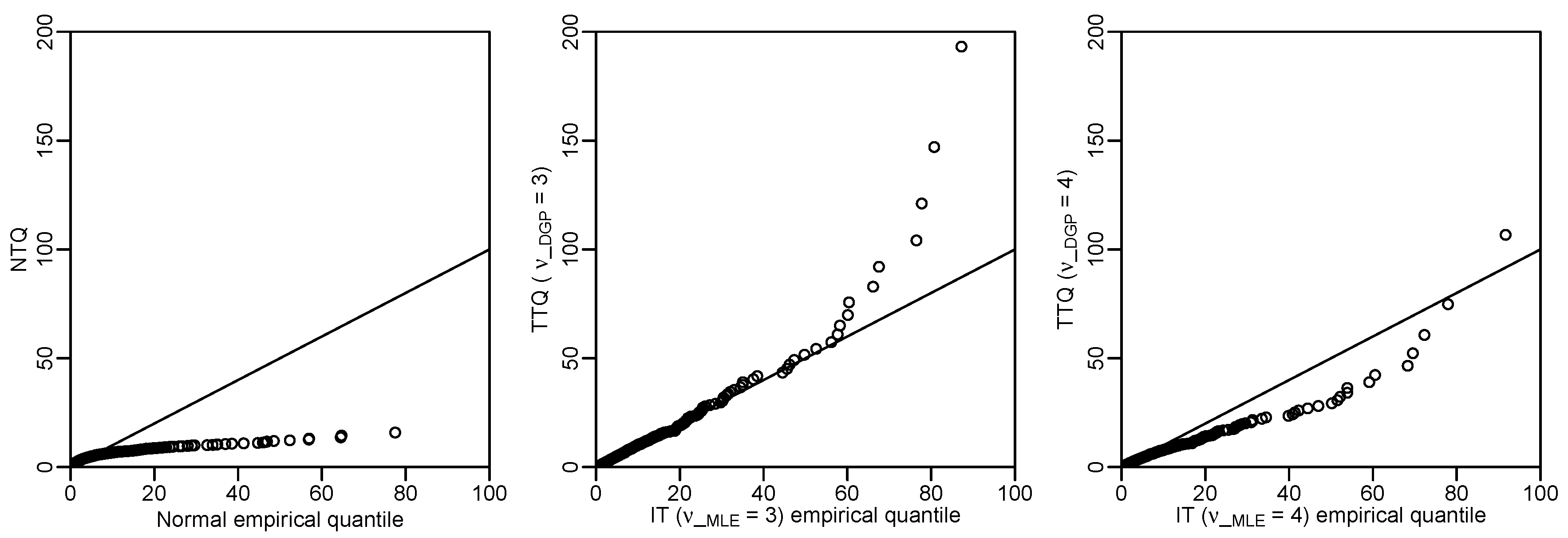
4.1. Distributions of Mahalanobis Distances
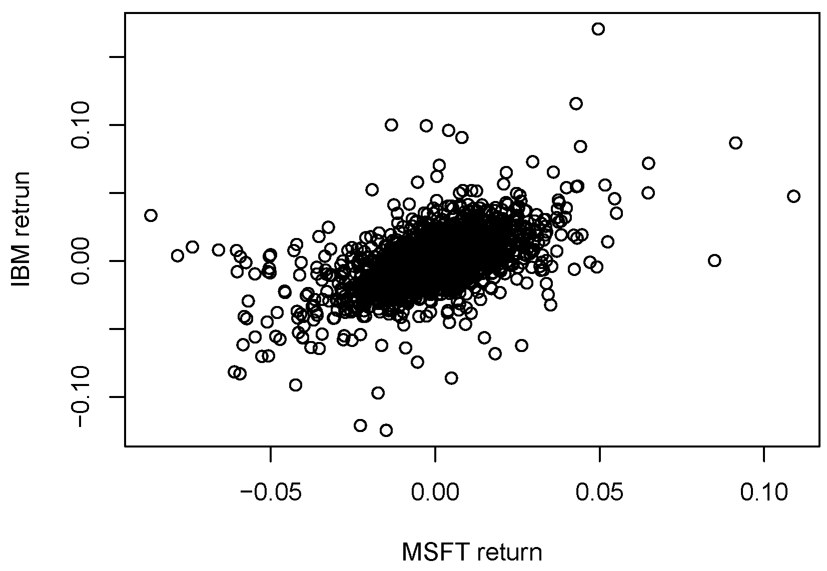
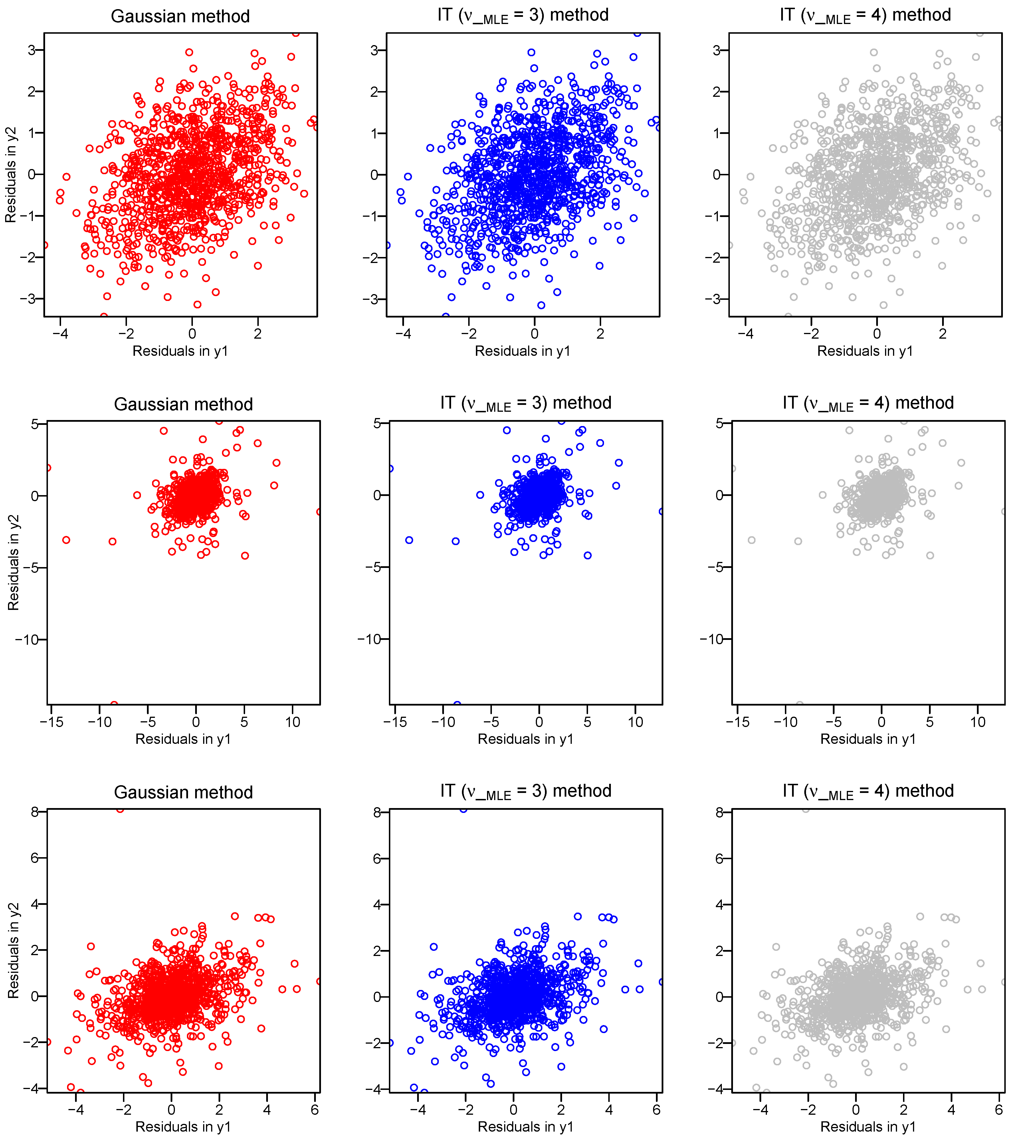
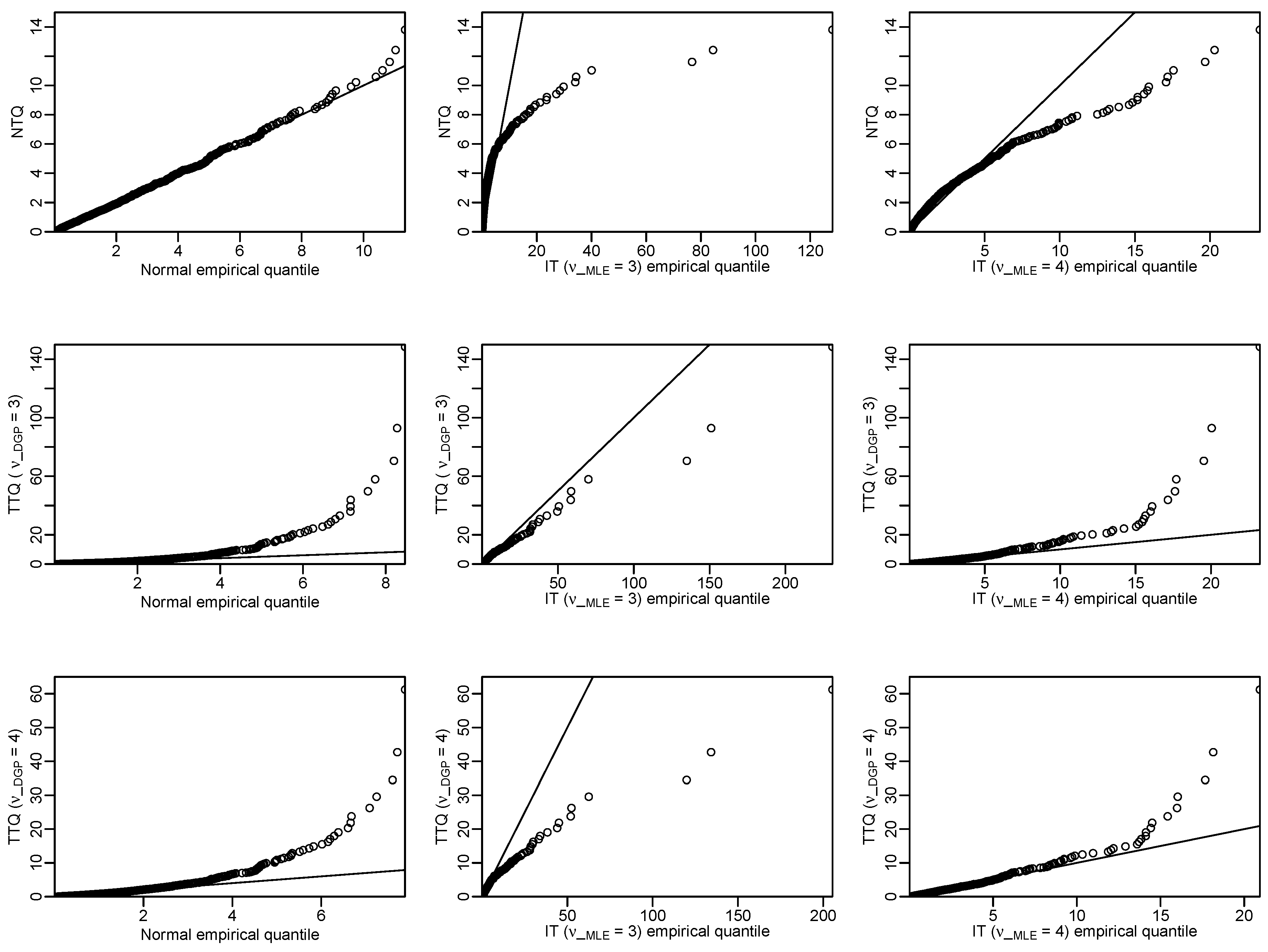
For an L-dimensional random vector Y , with mean μ , and covariance matrix Σ , the squared Mahalanobis distance is defined by:
d 2 = ( Y μ ) T Σ 1 ( Y μ )
If Y 1 , Y n is a sample of size n from the L-dimensional Gaussian distribution N L ( μ N , Σ N ) , the squared Mahalanobis distance of observation i, denoted by d N i 2 , follows a χ L 2 distribution. If μ N and Σ N are unknown, then the squared Mahalanobis distance of observation i can be estimated by:
d ^ N i 2 = ( Y i μ ^ N ) T Σ ^ N 1 ( Y i μ ^ N )
where μ ^ N = Y ¯ = 1 n i = 1 n Y i and Σ ^ N is the sample covariance matrix. The work in Gnanadesikan and Kettenring (1972) (see also Bilodeau and Brenner (1999)) proved that this square distance follows a Beta distribution, up to a multiplicative constant:
n ( n 1 ) 2 ( Y i μ ^ N ) T Σ ^ N 1 ( Y i μ ^ N ) B e t a L 2 , n L 1 2
where L is the dimension of Y . For large n, this Beta distribution can be approximated by the chi-square distribution d N i 2 χ L 2 . According to Gnanadesikan and Kettenring (1972) (p. 172), n = 25 already provides a sufficiently large sample for this approximation, which is the case in all our examples below. If we now assume that Y 1 , , Y n is a sample of size n from the L-dimensional Student distribution Y i T ( μ I T , Σ I T , ν ) , then the squared Mahalanobis distance of observation i, denoted by d I T i 2 and properly scaled, follows a Fisher distribution (see Roth (2013)):
1 L ν ν 2 d I T i 2 F ( L , ν )
If μ I T and Σ I T are unknown, then the squared Mahalanobis distance of observation i can be estimated by:
d ^ I T i 2 = ( Y i μ ^ I T ) T Σ ^ I T 1 ( Y i μ ^ I T ) ,
where μ ^ I T and Σ ^ I T are the MLE of μ I T and Σ I T . Note that in the IT model, μ ^ I T is no longer equal to Y ¯ . Up to our knowledge, there is no result about the distribution of d ^ I T i 2 .
In the elliptical distribution family, the distribution of Mahalanobis distances characterizes the distribution of the observations. Thus, in order to test the normality of the data, we can test whether the Mahalanobis distances follow a chi-square distribution. Similarly, testing the Student distribution is equivalent to testing whether the Mahalanobis distances follow the Fisher distribution. There are two difficulties with the approach. The first one is that the estimated Mahalanobis distances are not a sample from the chi-square (respectively, the Fisher) distribution because there is dependence due to the estimation of the parameters. The second one is that, in our case, we not only estimate μ and Σ , but we are in a regression framework where μ is linear combination of regressors, and we indeed estimate its coefficients. In what follows, we will ignore these two difficulties and consider that, for large n, the distributions of the estimated Mahalanobis distances behave as if μ and Σ were known.
We propose to implement several Kolmogorov–Smirnov tests in order to test different null hypothesis: Gaussian, Student with three degrees of freedom, and Student with four degrees of freedom. As an exploratory tool, we also propose drawing Q-Q plots of the Mahalanobis distances with respect to the chi-square and the Fisher distribution Small (1978).

4.2. Examples

This section illustrates some applications of the proposed methodology for selecting a model. We use a real dataset from finance and three simulated datasets with the same DGP as in Section 3.
The real dataset is the daily closing share price of IBM and MSFT, which are imported from Yahoo Finance from 3 January 2007–27 September 2018 using the quantmod package in R. It contains n = 2955 observations. Let S t , t = 1 , , n be the daily share price of IBM and MSFT and Y t be the log-price increment (return) (see Fung and Seneta (2010)) over a day period, then:
Y t = log S t log S t 1 .
The three other datasets are simulated using the same model as in Section 3 with the Gaussian DGP, the IT DGP with ν D G P = 3 , and the IT DGP with ν D G P = 4 and with sample size n = 1000 . Figure 2 (respectively, Figure 3) displays the scatterplots of the financial data (respectively, the three toy data).
We compute the Gaussian and the IT estimators as in Section 3. We then calculate the squared Mahalanobis distances of the residuals and use a Kolmogorov–Smirnov test for deciding between the models. For the financial data, we have no predictor. We test the Gaussian (respectively the Student with three degrees of freedom, the Student with four degrees of freedom) null hypothesis. When testing one of the null hypotheses, we use the estimator corresponding to the null. Moreover, when the null hypothesis is Student, we use the corresponding degrees of freedom for computing the maximum likelihood estimator. We do reject the null hypothesis if the p-value is smaller than α = 5 % . Note that we could adjust the level of α by taking into account multiple testing.
Table 8 shows the p-values of these tests. For the simulated data, at the 5 % level, we do not reject the Gaussian assumption when the DGP is Gaussian. Similarly, we do not reject the Student distribution with three (respectively, four) degrees of freedom when the DGP is the IT with degrees of freedom ν D G P = 3 (respectively, ν D G P = 4 ). For the financial data, we do not reject the Student distribution with three degrees of freedom, but we do reject the Gaussian distribution and the Student distribution with four degrees of freedom.
Figure 4 shows the Q-Q plots comparing the empirical quantiles of the Mahalanobis distances for the normal (respectively, the IT ( ν M L E = 3 ), the IT ( ν M L E = 4 )) estimators on the horizontal axis to the theoretical quantiles of the Mahalanobis distances for the normal (respectively, the IT ( ν M L E = 3 ), the IT ( ν M L E = 4 )) on the vertical axis for the financial data. These Q-Q plots are coherent with the results of the tests in Table 8. The IT model with three degrees of freedom fits our financial data well.
Figure 5 displays the Q-Q plots for the toy DGP: the Gaussian DGP in the first column, the IT DGP with ν D G P = 3 in the second column, and the IT DGP with ν D G P = 4 in the third column. The first row compares the empirical quantiles to the normal case quantiles, the second to the Student case quantiles with ν D G P = 3 , and the third row to Student case quantiles with ν D G P = 4 . The Q-Q plots on the diagonal confirm that the fit is good when the model is correct. The other Q-Q plots outside the diagonal correctly reveal a clear deviation from the hypothesized model.
To summarize the findings of this study, let us first say that there may be an abusive use of the Gaussian distribution in applications due to its simplicity. We have seen that considering the Student distribution instead is just slightly more complex, but feasible, and that one can test this choice. Concerning the two Student models, we have seen that the UT model is simpler to fit than the IT model, but has limitations due to the fact that it assumes a single realization, which restricts the properties of the maximum likelihood estimators and prevents the use of tests against the other two models.

5. Conclusions

We have compared three different models: the multivariate Gaussian model and two different multivariate Student models (uncorrelated or independent). We have derived some theoretical properties of the Student UT model and proposed a simple iterative reweighted algorithm to compute the maximum likelihood estimators in the IT model. Our simulations show that using a multivariate Student IT model instead of a multivariate Gaussian model for heavy tail data is simple and can be viewed as a safeguard against misspecification in the sense that there is more to loose if the DGP is Student and one uses a Gaussian model than in the reverse situation. Finally, we have proposed some graphical tools and a test to choose between the Gaussian and the IT models. The IT model fits our finance dataset quite well. There is still work to do in the direction of improving the model selection procedure to overcome the fact that the parameters are estimated and hence the hypothetical distribution is only approximate. Let us mention that it is also possible to adapt our algorithm for the IT model to the case of missing data. We intend to work in the direction of allowing different degrees of freedom for each coordinate. It may be also relevant to consider an alternative estimation method by generalizing the one proposed in Kent et al. (1994) to the multivariate regression case. Finally, another perspective is to consider multivariate errors-in-variables models, which allow incorporating measurement errors in the response and the explanatory variables. A possible approach is proposed in Croux et al. (2010).

Supplementary Materials

In order to allow the reproducibility of the empirical analyses contained in the present paper, some Supplementary Material is available at the following link: http://www.thibault.laurent.free.fr/code/jrfm/.

Author Contributions

T.H.A.N., C.T.-A. and A.R.-G., Methodology, analysis, review, and editing; T.H.A.N., writing, original draft preparation; C.T.-A. and A.R.-G. supervision and validation; T.L. and T.H.A.N., data curation.

Funding

This research received no external funding

Conflicts of Interest

The authors declare no conflict of interest.

Abbreviations

The following abbreviations are used in this manuscript:
EMExpectation-maximization
MLEMaximum likelihood estimator
NNormal (Gaussian) model
ITIndependent multivariate Student
UTUncorrelated multivariate Student
RBRelative bias
MSEMean squared error
RRMSERoot relative mean squared error
DGPData-generating process

Appendix A

Proof of Proposition 1.
Using Expression (1), the joint density function of ϵ ^ U T is:
p ( ϵ U T | 0 , Ω U T , ν ) = f ( ν ) det ( I n Σ U T ) 1 / 2 1 + 1 ν 2 ϵ U T T ( I n Σ U T ) 1 ϵ U T ν + n L 2 = f ( ν ) det ( Σ U T ) n / 2 1 + 1 ν 2 ϵ U T T ( I n Σ U T ) 1 ϵ U T ν + n L 2 = f ( ν ) det ( Σ U T ) n / 2 1 + 1 ν 2 i = 1 n ϵ U T i T Σ U T 1 ϵ U T i ν + n L 2
Therefore, the logarithm of p ( ϵ U T | 0 , Ω U T , ν ) is:
log p ( ϵ U T | 0 , Ω U T , ν ) = log f ( ν ) n 2 log Σ U T ν + n L 2 log 1 + 1 ν 2 i = 1 n ϵ U T i T Σ U T 1 ϵ U T i .
In order to maximize log p ( p ( ϵ U T | 0 , Ω U T , ν ) ) as a function of β U T , we follow the same argument as in Theorem 8.4 from Seber (2008) for the Gaussian case and obtain that the minimum of i = 1 n ϵ U T i T Σ U T 1 ϵ U T i is obtained for:
β ^ U T = X T X 1 X T Y .
Besides, taking the partial derivative of (A1) as a function of Σ U T , we obtain:
log ( p ( ϵ U T | 0 , Ω U T , ν ) ) Σ U T = n Σ U T 1 2 ( ν + n L ) 2 log ( ν 2 + i = 1 n ϵ U T i T Σ U T 1 ϵ U T i ) Σ U T = n Σ U T 1 2 ( ν + n L ) 2 ( ν 2 + i = 1 n ϵ U T i T Σ U T 1 ϵ U T i ) / Σ U T ν 2 + i = 1 n ϵ U T i T Σ U T 1 ϵ U T i .
Let:
w U T = 1 ν 2 + i = 1 n ϵ U T i T Σ U T 1 ϵ U T i .
We have:
log ( p ( ϵ U T | 0 , Ω U T , ν ) ) Σ U T = n Σ U T 1 2 ( ν + n L ) w U T 2 ( ν 2 + i = 1 n ϵ U T i T Σ U T 1 ϵ U T i ) / Σ U T = n Σ U T 1 2 + ( ν + n L ) w U T 2 i = 1 n Σ U T 1 ϵ U T i ϵ U T i T Σ U T 1
Solving log ( p ( ϵ U T | 0 , Ω U T , ν ) ) Σ U T = 0 and letting E = i = 1 n ϵ U T i ϵ U T i T , we have:
Σ U T 1 = ν + n L n w U T i = 1 n Σ U T 1 ϵ U T i ϵ U T i T Σ U T 1 Σ U T Σ U T 1 Σ U T = ν + n L n w U T i = 1 n Σ U T Σ U T 1 ϵ U T i ϵ U T i T Σ U T 1 Σ U T Σ U T = ( ν + n L ) w U T E n
The expression of w U T in (A3) can be simplified by noting that:
Σ U T 1 = n ( ( ν + n L ) w U T ) 1 E 1 i = 1 n ϵ U T i T Σ U T 1 ϵ U T i = n ( ( ν + n L ) w U T ) 1 i = 1 n ϵ U T i T E 1 ϵ U T i = n ( ν + n L ) w U T tr i = 1 n ϵ U T i ϵ U T i T E 1 i = 1 n ϵ U T i T Σ U T 1 ϵ U T i = n L ( ν + n L ) w U T .
Replacing the expression of i = 1 n ϵ U T i T Σ U T 1 ϵ U T i from (A4) into w U T , we get:
w U T = ν ( ν 2 ) ( ν + n L ) .
Finally,
Σ ^ U T = ν ν 2 i = 1 n ϵ ^ U T i ϵ ^ U T i T n .
Proof of Proposition 2.
The property E ( β ^ U T ) = β U T is immediate. In order to facilitate the derivation of the proof for Σ ^ U T , we write Model (4) as:
Y = X B + ε
where:
Y = y 11 y 12 y 1 L y n 1 y n 2 y n L , X = 1 x 11 x 1 K 1 x n 1 x n K , B = β 01 β 0 L β 11 β 1 L β K 1 β K L ε = ε 11 ε 12 ε 1 L ϵ n 1 ε n 2 ε n L , B ^ U T = ( X T X ) 1 X T Y and ε ^ U T = Y X B ^ U T .
Let E = ε ^ U T T ε ^ U T and M = I n X ( X T X ) 1 X T . We have M X B = 0 , and following Seber (2008), Theorem 8.2,
E = ( Y X B ^ U T ) T ( Y X B ^ U T ) = ( M Y ) T M Y = Y T M Y = ( Y X B ) T M ( Y X B ) = ε T M ε = h i M h i ε h ε i T .
Since E ( ε h ε i T ) = Σ if   h = i 0 otherwise , for h , i = 1 , , n , E ( E ) = h M h h Σ = t r ( M ) Σ = ( n K ) Σ and:
E ( Σ ^ U T ) = E ν ν 2 E n = ν ν 2 E ( E ) n = ν ν 2 n K n Σ U T .

References

  1. Bilodeau, Martin, and David Brenner. 1999. Theory of Multivariate Statistics (Springer Texts in Statistics). Berlin: Springer, ISBN 978-0-387-22616-3. [Google Scholar]
  2. Croux, Christophe, Mohammed Fekri, and Anne Ruiz-Gazen. 2010. Fast and robust estimation of the multivariate errors in variables model. Test 19: 286–303. [Google Scholar] [CrossRef]
  3. Dempster, Arthur P., Nan M. Laird, and Donald B. Rubin. 1978. Iteratively Reweighted Least Squared for Linear Regression when Errors are Normal/Independent distributed. Multivariate Analysis V 5: 35–37. [Google Scholar]
  4. Dogru, Fatma Zehra, Y. Murat Bulut, and Olcay Arslan. 2018. Double Reweighted Estimators for the Parameters of the Multivariate t distribution. Communications in Statistics-Theory and Methods 47: 4751–71. [Google Scholar] [CrossRef]
  5. Fernandez, Carmen, and Mark F. J. Steel. 1999. Multivariate Student t- Regression Models: Pitfalls and Inference. Biometrika Trust 86: 153–67. [Google Scholar] [CrossRef]
  6. Fung, Thomas, and Eugene Seneta. 2010. Modeling and Estimating for Bivariate Financial Returns. International Statistical Review 78: 117–33. [Google Scholar] [CrossRef]
  7. Fraser, Donald Alexander Stuart. 1979. Inference and Linear Models. New York: McGraw Hill, ISBN 9780070219106. [Google Scholar]
  8. Fraser, Donald Alexander Stuart, and Kai Wang Ng. 1980. Multivariate regression analysis with spherical error. Multivariate Analysis 5: 369–86. [Google Scholar]
  9. Gnanadesikan, Ram, and Jon R. Kettenring. 1972. Robust estimates, residuals, and outlier detection with multiresponse data. Biometrics 28: 81–124. [Google Scholar] [CrossRef]
  10. Hofert, Marius. 2003. On Sampling from the Multivariate t Distribution. The R Journal 5: 129–36. [Google Scholar] [CrossRef]
  11. Hu, Wenbo, and Alec N. Kercheval. 2009. Portfolio optimization for Student t and skewed t returns. Quantitative Finance 10: 129–36. [Google Scholar] [CrossRef]
  12. Huber, Peter J., and Elvezio M. Ronchetti. 2009. Robust Statistics. Hoboken: Wiley, ISBN 9780470129906. [Google Scholar]
  13. Johnson, Norman L., and Samuel Kotz. 1972. Student multivariate distribution. In Distribution in Statistics: Continuous Multivariate Distributions. Michigan: Wiley Publishing House, ISBN 9780471443704. [Google Scholar]
  14. Kan, Raymond, and Guofu Zhou. 2017. Modeling non-normality using multivariate t: implications for asset pricing. China Finance Review International 7: 2–32. [Google Scholar] [CrossRef]
  15. Katz, Jonathan N., and Gary King. 1999. A Statistical Model for Multiparty Electoral Data. American Political Science Review 93: 15–32. [Google Scholar] [CrossRef]
  16. Kelejian, Harry H., and Ingmar R. Prucha. 1985. Independent or Uncorrelated Disturbances in Linear Regression. Economics Letters 19: 35–38. [Google Scholar] [CrossRef]
  17. Kent, John T., David E. Tyler, and Yahuda Vard. 1994. A curious likelihood identity for the multivariate t-distribution. Communications in Statistics-Simulation and Computation 23: 441–53. [Google Scholar] [CrossRef]
  18. Kotz, Samuel, and Saralees Nadarajah. 2004. Multivariate t Distributions and Their Applications. Cambridge: Cambridge University Press, ISBN 9780511550683. [Google Scholar]
  19. Lange, Kenneth, Roderick J. A. Little, and Jeremy Taylor. 1989. Robust Statistical Modeling Using the t-Distribution. International Statistical Review 84: 881–96. [Google Scholar] [CrossRef]
  20. Lange, Kenneth, and Janet S. Sinsheimer. 1993. Normal/Independent Distributions and Their Applications in Robust Regression. Journal of Computational and Graphical Statistics 2: 175–98. [Google Scholar] [CrossRef]
  21. Liu, Chuanhai, and Donald B. Rubin. 1995. ML estimation of the t distribution using EM and its extensions, ECM and ECME. Statistica Sinica 5: 19–39. [Google Scholar]
  22. Liu, Chuanhai. 1997. ML Estimation of the Multivariate t Distribution and the EM Algorithm. J. Multivar. Anal. 63: 296–312. [Google Scholar] [CrossRef]
  23. Maronna, Ricardo Antonio. 1976. Robust M-Estimators of Multivariate Location and Scatter. The Annals of Statistics 4: 51–67. [Google Scholar] [CrossRef]
  24. McNeil, Alexander J., Rüdiger Frey, and Paul Embrechts. 2005. Quantitative Risk Management: Concepts, Techniques and Tools. Vol. 3, Princeton: Princeton University Press. [Google Scholar]
  25. Platen, Eckhard, and Renata Rendek. 2008. Empirical Evidence on Student-t Log-Returns of Diversified World Stock Indices. Journal of Statistical Theory and Practice 2: 233–51. [Google Scholar] [CrossRef]
  26. Prucha, Ingmar R., and Harry H. Kelejian. 1984. The Structure of Simultaneous Equation Estimators: A generalization Towards Nonnormal Disturbances. Econometrica 52: 721–36. [Google Scholar] [CrossRef]
  27. Roth, Michael. 2013. On the Multivariate t Distribution. Report Number: LiTH-ISY-R-3059. Linkoping: Department of Electrical Engineering, Linkoping University. [Google Scholar]
  28. Seber, George Arthur Frederick. 2008. Multivariate Observations. Hoboken: John Wiley & Sons, ISBN 9780471881049. [Google Scholar]
  29. Singh, Radhey. 1988. Estimation of Error Variance in Linear Regression Models with Errors having Multivariate Student t-Distribution with Unknown Degrees of Freedom. Economics Letters 27: 47–53. [Google Scholar] [CrossRef]
  30. Small, N. J. H. 1978. Plotting squared radii. Biometrics 65: 657–58. [Google Scholar] [CrossRef]
  31. Sutradhar, Brajendra C., and Mir M. Ali. 1986. Estimation of the Parameters of a Regression Model with a Multivariate t Error Variable. Communication Statistics Theory and Method 15: 429–50. [Google Scholar] [CrossRef]
  32. Zellner, Arnold. 1976. Bayesian and Non-Bayesian Analysis of the Regression Model with Multivariate Student-t Error Terms. Journal of the American Statistical Association 71: 400–5. [Google Scholar] [CrossRef]
Figure 1. The RRMSE of the IT estimator of β ^ 12 for the UT DGP in solid line, for the IT DGP in dashed line, and for the Gaussian DGP in dotted line with ν D G P = 3 (respectively, ν D G P = 4 , ν D G P = 5 ) on the left (respectively, middle, right) plot.
Jrfm 12 00028 g001
Figure 2. Financial data: scatterplot of returns.
Jrfm 12 00028 g002
Figure 3. Toy data: scatterplots of residuals in the Gaussian DGP (respectively, the IT DGP with ν D G P = 3 , the IT DGP with ν D G P = 4 ) on the first row (respectively, the second row, the third row).
Jrfm 12 00028 g003
Figure 4. Financial data: Q-Q plots of the Mahalanobis distances for the normal, IT ( ν M L E = 3 ), and IT ( ν M L E = 4 ) estimators.
Jrfm 12 00028 g004
Figure 5. Toy data: Q-Q plots of the Mahalanobis distances of the residuals for the normal (respectively, the IT with ν D G P = 3 , the IT with ν D G P = 4 ) case empirical quantiles against the normal (respectively, the IT with ν M L E = 3 , the IT with ν M L E = 4 ) case theoretical quantiles in the first row (respectively, the second row, the third row).
Jrfm 12 00028 g005
Table 1. Distribution of the error vector ϵ in the Gaussian, UT, and IT models.
ModelDistribution
N ( ϵ 1 , , ϵ n ) N n L ( 0 , I n Σ N ) = i = 1 n N L ( 0 , Σ N )
UT ( ϵ 1 , , ϵ n ) T n L ( 0 , I n Σ U T , ν )
IT ( ϵ 1 , , ϵ n ) i = 1 n T L ( 0 , Σ I T , ν )
Table 2. Relative bias and relative root mean squared error of the estimators of β ( β ^ N , β ^ U T , β ^ I T ) for the corresponding DGP (Gaussian, UT, and IT).
DGPNUT ( ν DGP = 3 )IT ( ν DGP = 3 )
MethodsEstimatorsRB (%)RRMSERB (%)RRMSERB (%)RRMSE
β ^ N , β ^ U T β ^ 01 −0.071.00−0.061.00−0.091.48
β ^ 02 0.001.000.001.000.001.48
β ^ 11 −0.021.00−0.011.00−0.071.46
β ^ 12 −0.001.00−0.001.00−0.001.46
β ^ I T ( ν M L E = 3 ) β ^ 01 −0.091.04−0.091.09−0.031.00
β ^ 02 0.001.040.001.090.001.00
β ^ 11 −0.041.07−0.021.08−0.031.00
β ^ 12 −0.001.07−0.001.08−0.001.00
Table 3. Bias and MSE of the maximum likelihood estimators of β for the corresponding DGP (Gaussian, UT, and IT).
DGPNUT ( ν DGP = 3 )IT ( ν DGP = 3 )
EstimatorsBiasMSEBiasMSEBiasMSE
β ^ 01 1.39 × 10 3 4.57 × 10 2 1.27 × 10 3 3.72 × 10 2 6.65 × 10 4 1.99 × 10 2
β ^ 02 2.41 × 10 5 2.18 × 10 5 1.47 × 10 5 1.76 × 10 5 9.90 × 10 6 9.50 × 10 6
β ^ 11 6.62 × 10 4 2.16 × 10 2 3.23 × 10 4 2.05 × 10 2 1.02 × 10 3 9.84 × 10 3
β ^ 12 1.87 × 10 5 1.02 × 10 5 3.90 × 10 6 9.60 × 10 6 2.14 × 10 5 4.70 × 10 6
Table 4. The root relative mean squared errors of β ^ .
MethodsDGPNUTIT
RRMSE ν DGP = 3 ν DGP = 4 ν DGP = 5 ν DGP = 3 ν DGP = 4 ν DGP = 5
N β ^ 01 1.001.001.001.001.481.221.14
β ^ 02 1.001.001.001.001.481.231.14
β ^ 11 1.001.001.001.001.461.221.13
β ^ 12 1.001.001.001.001.461.221.13
IT ( ν M L E = 3 ) β ^ 01 1.041.091.091.081.001.001.01
β ^ 02 1.041.091.091.081.001.001.01
β ^ 11 1.071.081.101.081.001.001.01
β ^ 12 1.071.081.091.091.001.001.01
IT ( ν M L E = 4 ) β ^ 01 1.021.071.061.061.001.001.00
β ^ 02 1.011.061.061.051.001.001.00
β ^ 11 1.041.061.071.061.001.001.00
β ^ 12 1.041.051.071.061.001.001.00
IT ( ν M L E = 5 ) β ^ 01 1.001.051.051.041.011.001.00
β ^ 02 1.001.051.051.041.011.001.00
β ^ 11 1.031.041.051.051.011.001.00
β ^ 12 1.031.041.051.051.011.001.00
Table 5. The bias and the MSE of ρ ^ , σ ^ 1 2 , σ ^ 2 2 .
MethodsDGPNUT ( ν DGP = 3 )IT ( ν DGP = 3 )
BiasMSEBiasMSEBiasMSE
N ρ ^ 4.85 × 10 4 9.46 × 10 4 2.08 × 10 4 7.68 × 10 4 3.99 × 10 3 1.17 × 10 2
σ ^ 1 2 3.89 × 10 3 8.33 × 10 3 1.05 × 10 1 58 6.94 × 10 3 3.17
σ ^ 2 2 1.75 × 10 3 2.01 × 10 3 5.17 × 10 2 14.93 1.77 × 10 2 2.85 × 10 1
IT
ν M L E = 3
ρ ^ 1.70 × 10 4 8.94 × 10 4 2.18 × 10 4 9.05 × 10 4 2.03 × 10 4 1.07 × 10 3
σ ^ 1 2 2.00 4.06 1.80 244.87 1.43 × 10 2 1.54 × 10 2
σ ^ 2 2 1.00 1.02 0.91 64.75 7.30 × 10 3 3.94 × 10 3
Table 6. The RB of ρ ^ , σ ^ 1 2 , σ ^ 2 2 with ν = 3 , 4 , 5 .
MethodsDGPNUTIT
RB (%) ν DGP = 3 ν DGP = 4 ν DGP = 5 ν DGP = 3 ν DGP = 4 ν DGP = 5
N ρ ^ −0.14−0.06−0.06−0.06−1.13−0.240.02
σ ^ 1 2 −0.21−5.23−3.34−2.310.35−0.08−0.12
σ ^ 2 2 −0.18−5.17−3.33−2.20−1.77−0.30−0.09
IT, ν M L E = 3 ρ ^ −0.05−0.06−0.06−0.06−0.06−0.04−0.02
σ ^ 1 2 99.9990.2593.8995.80−0.7232.7950.12
σ ^ 2 2 100.0590.6093.9096.03−0.7332.7950.13
IT, ν M L E = 4 ρ ^ −0.05−0.06−0.06−0.06−0.06−0.04−0.01
σ ^ 1 2 42.6235.8038.3239.68−24.66−0.2411.18
σ ^ 2 2 42.6636.0138.3439.85−24.67−0.2311.19
IT, ν M L E = 5 ρ ^ −0.06−0.06−0.06−0.06−0.06−0.04−0.00
σ ^ 1 2 24.7118.8521.0322.23−31.75−10.13−0.14
σ ^ 2 2 24.7419.0221.0422.38 3 1.76−10.13−0.14
Table 7. The RRMSE of ρ ^ , σ ^ 1 2 , σ ^ 2 2 in the Gaussian DGP, the UT DGP ( ν DGP = 3 , 4 , 5 ), and the IT DGP ( ν DGP = 3 , 4 , 5 ).
MethodsDGPNUTIT
RRMSE ν DGP = 3 ν DGP = 4 ν DGP = 5 ν DGP = 3 ν DGP = 4 ν DGP = 5
N ρ ^ 1.001.001.001.003.211.911.42
σ ^ 1 2 1.001.001.001.0014.332.651.64
σ ^ 2 2 1.001.001.001.008.502.241.78
IT, ν M L E = 3 ρ ^ 0.971.091.091.091.001.001.01
σ ^ 1 2 22.072.052.112.161.005.899.18
σ ^ 2 2 22.452.082.112.161.005.779.13
IT, ν M L E = 4 ρ ^ 0.951.061.061.061.011.001.00
σ ^ 1 2 9.491.461.471.484.041.002.31
σ ^ 2 2 9.651.481.471.484.001.002.30
IT, ν M L E = 5 ρ ^ 0.941.051.051.051.011.001.00
σ ^ 1 2 5.581.271.271.285.161.991.00
σ ^ 2 2 5.681.281.281.275.101.951.00
Table 8. All datasets: the p-values of the Mahalanobis distances tests with the null hypothesis and the corresponding estimators.
Hypothesis H 0 Toy DGPFinancial Data
MethodsNIT, ν DGP = 3 IT, ν DGP = 4
N0.546 2.2 × 10 16 2.2 × 10 16 2.2 × 10 16
IT, ν M L E = 3 2.2 × 10 16 0.4050.0330.882
IT, ν M L E = 4 2.2 × 10 16 0.0230.3030.049

