Hyperspectral Image Denoising Based on Spectral Dictionary Learning and Sparse Coding

Abstract

Processing and applications of hyperspectral images (HSI) are limited by the noise component. This paper establishes an HSI denoising algorithm by applying dictionary learning and sparse coding theory, which is extended into the spectral domain. First, the HSI noise model under additive noise assumption was studied. Considering the spectral information of HSI data, a novel dictionary learning method based on an online method is proposed to train the spectral dictionary for denoising. With the spatial–contextual information in the noisy HSI exploited as a priori knowledge, the total variation regularizer is introduced to perform the sparse coding. Finally, sparse reconstruction is implemented to produce the denoised HSI. The performance of the proposed approach is better than the existing algorithms. The experiments illustrate that the denoising result obtained by the proposed algorithm is at least 1 dB better than that of the comparison algorithms. The intrinsic details of both spatial and spectral structures can be preserved after significant denoising.

1. Introduction

Hyperspectral images (HSIs) are widely used in military, geological exploration, forestry, and agriculture domains as entry data [1,2]. Information contained in HSI can be decomposed into either unidimensional data, representing the spectral information, or bi-dimensional data, representing the spatial information. In real-world applications, the processing of HSI often includes unmixing [3,4], classification [5,6], and target detection [7,8]. However, the nature of HSI acquisition inevitably results in the blending of noise in HSI data. The noise information not only reduces the visual quality of images, but also complicates the processing of HSI, so the results of processing are less accurate [9]. Thus, HSI denoising is the first and a crucial phase of HSI processing, necessitating research for more effective and economic denoising methods. This domain has gained popularity, attracting many researchers [10].

In the research of HSI denoising methods, various theories have been proposed and tested. Initially, since each spectral channel in the HSI data cube can be treated as a grey-level image, typical two-dimensional (2D) image denoising algorithms, such as block-matching three-dimensional (3D) filtering (BM3D) [11], total variation (TV) [12], and the nonlocal-based algorithm [13], were applied to denoise HSIs band-by-band. Then, some denoising methods conceived for 3D data, such as video denoising by sparse 3D transform-domain collaborative filtering (VBM3D) [14] and block-matching four-dimensional (4D) filtering (BM4D) [15], were applied to HSIs. However, the above denoising methods fail to consider the high correlation between spectral bands and always produce low-quality results. To take advantage of the correlation between spectral dimensions, a principal component analysis (PCA) combined with the block-matching 4D filtering method (PCA + BM4D) was proposed in Reference [16]. Since adjacent pixels in HSIs are highly correlated, HSIs exhibit a low-rank structure. Through investigating the low-rank property of HSIs, some denoising methods under low-rank-based frameworks have been proposed, such as low-rank matrix recovery (LRMR) [17] and a noise-adjusted iterative low-rank matrix approximation (NAILRMA) [18]. Notably, the high-level noise intensity in HSIs may affect the quality of denoising results obtained by low-rank-based methods.

With many applications in the field of image and signal processing, sparse representation performs better and continues to attract researchers’ attention [19]. Thus, sparse representation has been introduced into image denoising problems [20]. Since natural images or signals have a low-rank property [21], the latent clean image or signal is assumed to be a linear combination of basis vectors from a specific dictionary. In this assumption, noise is random and cannot be represented by any basic vector in the dictionary. Therefore, the noise component can be significantly reduced by projecting the image onto a subspace formed by the dictionary. In this theory, image denoising is the sparse signal recovery task supported by a specific dictionary.

In order to solve the HSI denoising problem better, Zhang [22] stated that the high-precision sparse reconstruction optimization can be realized by constructing an appropriate dictionary from the noisy image. Through work on dictionary learning, several methods employed to train the dictionary with the noisy image have been introduced. Among them, Elad and Aharon [23] proposed the typical K-means singular value decomposition (K-SVD) algorithm to manage the image denoising problem. The K-SVD algorithm obtains an overcomplete dictionary using a preliminary training process. In K-SVD dictionary learning, sparse coding is performed by block coordinate relaxation (BCR) in each iteration, and the dictionary update is performed by eigenvalue decomposition. To minimize the objective function under certain constraints, each iteration of the dictionary learning needs to access all the elements in the training set, which is a batch method based on the second iteration. Thus, K-SVD has a high computational complexity and application to large-scale datasets like HSIs is difficult. K-SVD operates under the assumption that the exact noise variance is already known. In real life, the accuracy of image restoration is quite sensitive to the error of the estimated variance [20]. Zhou [20] proposed a nonparametric Bayesian dictionary learning method and applied it to HSI denoising. In this algorithm, dictionary learning is regarded as a factor analysis problem in which the factor loading corresponds to a dictionary atom, and potential correlation between spectral bands is adaptively considered by using beta process factor analysis (BPFA). The adaptive dictionary update is performed by applying Gibbs sampling to the noisy image and manifesting an approximation to the complete posterior probability. BPFA takes advantage of the correlation between spectral bands in the noisy HSI and produces a good denoising result. However, BPFA needs to access all the elements in the training datasets for each iteration, resulting in a high computational complexity, and requires variance in noise or residual as a priori knowledge. On the basis of BPFA, Shen [24] proposed an adaptive spectrum-weighted sparse Bayesian dictionary learning method (ABPFA). Under the compressed sensing framework, the correlation between spectral bands in the noisy HSI was adaptively considered using beta process factor analysis. Since the method was an improvement on BPFA, it has the same disadvantages as the method.

In order to obtain a dictionary with a better training efficiency, an online dictionary learning algorithm (ODL) was proposed by Mairal et al. [25]. ODL selects only one subset or element from the training dataset each iteration, which is an effective statistical approximation of the batch method. This dictionary learning strategy can produce a dictionary that is adapted to the image in question by minimizing representation error, and improves the accuracy of the denoising of this [26]. Hao [27] introduced the ODL to the complex domain to solve the denoising problem of interferometric synthetic aperture radar (SAR) images.

Considering the large scale of HSIs, we use the online method to construct an adaptive dictionary from noisy HSI for denoising. Due to the special imaging model, hyperspectral data are a three-dimensional (3D) cube. Since the dictionary learning algorithms are initially applied to 2D images, they similarly manage the hyperspectral data. After expanding the noisy hyperspectral data cube into a pixel spectral matrix, dictionary learning algorithms select blocks in the matrix as the training set to obtain dictionary atoms. However, the spectral information of hyperspectral data cannot be fully utilized with this method. Therefore, we use the pixel spectral vectors instead of the traditional image blocks as the training data to perform dictionary learning. Obviously, the learned dictionary dimension is the same as the HSI spectral dimension. Under the linear mixture model (LMM), the dictionary atoms are regarded as spectral curves constituting the noisy HSI. Thereby, the dictionary atoms can better reflect the details of spectral features, and more precise HSI sparse reconstruction optimization can be realized, which means better denoising results.

The HSI denoising algorithm proposed in this study is based on sparse coding and adaptive dictionary learning, which is termed HyDeSpDLS. In the denoising algorithm, we propose a novel approach for directly constructing a dictionary from hyperspectral data by progressively using the pixel spectral vectors as the training set. Compared with overall loading methods, such as the batch method, the proposed dictionary learning approach can significantly improve the training efficiency, and the learned dictionary can adaptively represent HSIs. With the learned dictionary, the sparse coding is performed using a variable splitting and augmented Lagrangian and total variation method. The total variation regularization is spatially homogenous, which means that nearby pixels have similar coefficients for the same endmember. As a priori knowledge, the total variation regularizer improves the sparse reconstruction accuracy. These improvements make HyDeSpDLS a competitive HSI denoiser.

This paper has the following contributions:

(1)

The proposed novel dictionary learning method can construct a dictionary directly from noisy HSIs. To adopt the characteristics of HSI data, we use an online method to improve the training efficiency and use the pixel spectral vectors instead of the traditional image blocks as the training dataset to fully use the spectral information in noisy HSIs.

(2)

Considering the spatial-contextual information in HSI data, the TV regularizer is introduced into the sparse coding after the dictionary is obtained to guarantee that neighboring pixels have similar coefficients for one same endmember. With this prior information, the accuracy of sparse reconstruction improves.

This work is an extension of a conference paper [28]. The new material is as follows:

(1)

The online spectral dictionary learning algorithm is introduced and characterized in detail.

(2)

Considering the spatial-contextual information, a new algorithm is introduced to perform the sparse representation, termed sparse regression by variable splitting and augmented Lagrangian and total variation (SpaRSAL-TV).

(3)

More exhaustive experiments and comparisons are listed.

The contents of this paper are divided into five parts. The first part briefly introduces the background and current status of the research topic. The second part presents the mathematical noise model and the theory of HSI denoising. In the third part, the sparse coding method and the dictionary learning algorithm are explained. The fourth part formally outlines HyDeSpDLS, a denoising approach based on online dictionary learning and sparse representation in the spectral domain. The fifth part presents the results of the proposed method when applied to real and synthetic data, which are compared with the denoising methods produced by other authors. The final part concludes this paper.

2. HSI Noise Model and Denoising Mechanism

2.1. HSI Noise Model

Under the additive noise assumption, the HSI noise model is written as below:

$$\mathit{f}=\mathit{s}+\mathit{n}$$

(1)

where $\mathit{s}=\left[{\mathit{s}}_1,{\mathit{s}}_2,\dots ,{\mathit{s}}_L\right]$ is the original clean HSI, and its size is $M\times N\times L$; $M$ is the number of samples in a single scan; $N$ is the scan number in the image; $L$ is the band number; $\mathit{f}=\left[{\mathit{f}}_1,{\mathit{f}}_2,\dots ,{\mathit{f}}_L\right]$ is the noisy image, sized $M\times N\times L$; and $\mathit{n}=\left[{\mathit{n}}_1,{\mathit{n}}_2,\dots ,{\mathit{n}}_L\right]$ is the additive noise, and its size is $\mathit{f}$.

The above noise model indicates that HSI denoising is actually the estimation of the potential clean image $\mathit{s}$ based on the prior knowledge of the noise image $\mathit{f}$.

In practical applications, the hyperspectral data cube is usually expanded by scan lines into a matrix form composed of pixel spectral vectors as $\mathit{X}=\left[{\mathit{x}}_1,{\mathit{x}}_2,\dots ,{\mathit{x}}_n\right]\in {\mathbf{R}}^{L\times n}$, where $n$ is the number of pixel spectral vectors and $n$ is equal to the product of $M$ and $N$. Therefore, in hyperspectral denoising, according to an additive noise assumption, we write the observation model as follows:

$$\mathit{Y}=\mathit{X}+\mathit{N}$$

(2)

where $\mathit{Y},\mathit{N}\in {\mathbf{R}}^{L\times n}$ are the observed HSI data and the observed noise, respectively; and $\mathit{Y}=\left[{\mathit{y}}_1,{\mathit{y}}_2,\dots ,{\mathit{y}}_n\right]\in {\mathbf{R}}^{L\times n}$.

2.2. Denoising Process

HSI obtained in the real world is usually noisy, which means that the image can be considered decomposition of a random noise component and a clean image, which can be further decomposed using a dictionary. A clean image is a small number of basis vectors extracted from a dictionary, called a linear combination of atoms. In this assumption, noise is random and cannot be represented by any basic vector in the dictionary. Therefore, noise can be efficiently reduced by reconstructing the image with a dictionary and the corresponding sparse codes.

Considering the special structure of HSI data, constructing a dictionary in the spectral domain to sparsely represent images is more consistent with the imaging mode and physical meaning of HSIs. Since the number of bands contained in an image is usually as high as several hundreds, it is more efficient and time-efficient to perform HSI denoising with a pixel spectral matrix expanded from the data cube.

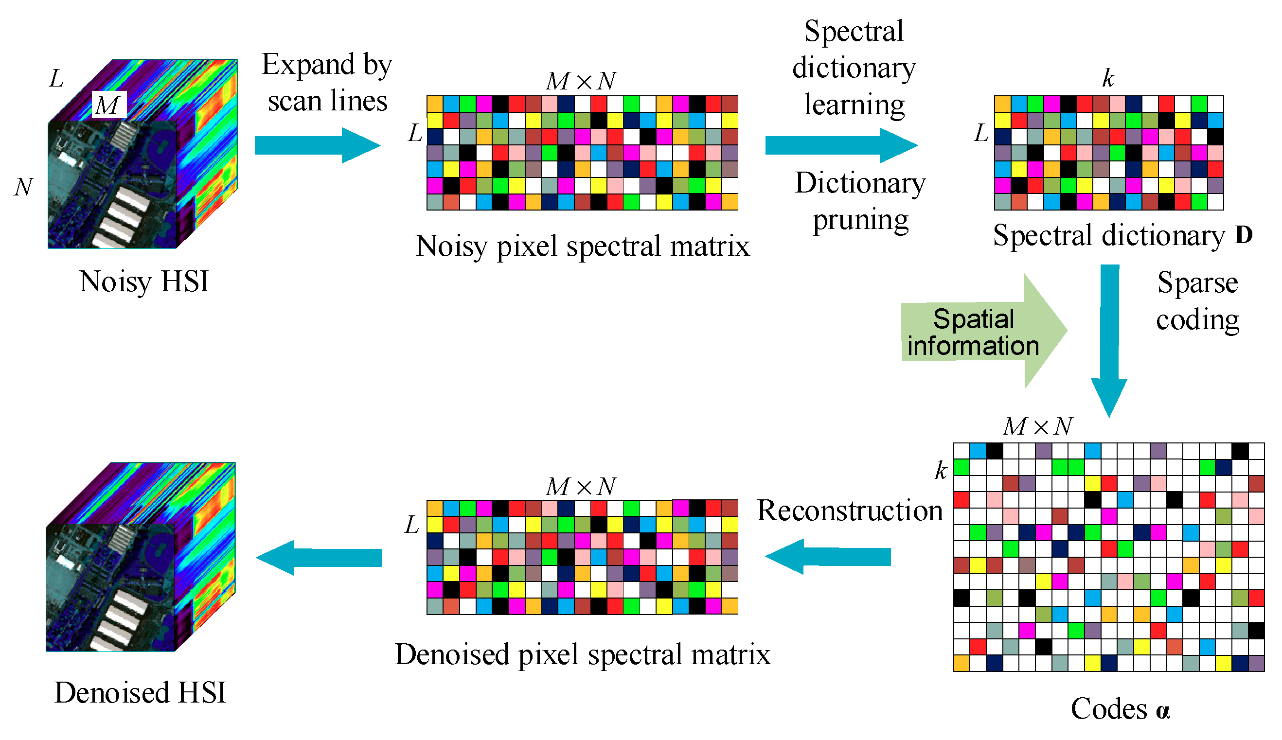
Therefore, we expand the noisy HSI by scan lines into a pixel matrix, which is used as a training set so that a spectral dictionary can be obtained. The noisy image can be reconstructed with the dictionary and the corresponding sparse codes. The denoising process is shown in Figure 1.

2.3. Denoising Mechanism

According to the above analysis of the HSI noise model and the denoising process, HSI denoising can be regarded as a sparse signal recovery task supported by a specific dictionary.

Considering the sparse property of HSIs, the clean HSI may be represented as:

$$\mathit{X}=\mathit{D}\mathit{\alpha }$$

(3)

where $\mathit{D}\in {\mathbf{R}}^{L\times k}$ represents the spectral dictionary, $k$ is the number of dictionary atoms, $\mathit{\alpha }\in {\mathbf{R}}^{k\times n}$ denotes the sparse codes, and only a few elements in each column are nonzero.

Then, Equation (2) can be written as:

$$\mathit{Y}=\mathit{D}\mathit{\alpha }+\mathit{N}$$

(4)

Therefore, the HSI denoising problem is formulated as:

$$\underset{\mathit{\alpha }}{\min }\frac{1}{2}{\Vert \mathit{D}\mathit{\alpha }-\mathit{Y}\Vert }_F^2+\lambda \cdot \varphi \left(\mathit{\alpha }\right)$$

(5)

where, ${\Vert \mathit{D}\mathit{\alpha }-\mathit{Y}\Vert }_F=\sqrt{\mathrm{trace}\left(\left(\mathit{D}\mathit{\alpha }-\mathit{Y}\right){\left(\mathit{D}\mathit{\alpha }-\mathit{Y}\right)}^{\mathrm{T}}\right)}$ is the Frobenius norm of $\mathit{D}\mathit{\alpha }-\mathit{Y}$.

For the pixel spectral vector $i$, Equation (4) can be written as:

$${\mathit{y}}_i=\mathit{D}{\mathit{\alpha }}_i+{\mathit{n}}_i$$

(6)

where ${\mathit{y}}_i\in {\mathbf{R}}^L,i=1,2,\dots ,n$ represents the observed pixel spectral vector, ${\mathit{n}}_i\in {\mathbf{R}}^L$ represents the corresponding noise components, and ${\mathit{\alpha }}_i\in {\mathbf{R}}^k$ denotes the corresponding sparse codes vector.

Then, the optimization in Equation (5) can be written as:

$$\underset{{\mathit{\alpha }}_i}{\min }\frac{1}{2}{\Vert \mathit{D}{\mathit{\alpha }}_i-{\mathit{y}}_i\Vert }_2^2+\lambda {\Vert {\mathit{\alpha }}_i\Vert }_0$$

(7)

where ${\Vert {\mathit{\alpha }}_i\Vert }_0$ is the nonzero element number of vector ${\mathit{\alpha }}_i$, which is termed as a $l_0$ norm, and the regularization parameter $\lambda$ (>0) is used to establish the relative weight between the two terms in the objective function.

Since the optimization problem of the $l_0$ norm is non-convex, the problem is hard to precisely and easily solve. The $l_0$ norm can be replaced with the $l_1$ norm as a convex approximation to deal with the optimization in Equation (7). Then, Equation (7) can be written as a constrained sparse regression:

$$\underset{{\mathit{\alpha }}_i}{\min }{\Vert {\mathit{\alpha }}_i\Vert }_1\mathrm{s}.\mathrm{t}.{\Vert \mathit{D}{\mathit{\alpha }}_i-{\mathit{y}}_i\Vert }_2^2\le \delta$$

(8)

where $\delta \ge 0$ is the parameter controlling the reconstruction error.

To obtain the sparse codes ${\widehat{\mathit{\alpha }}}_i$ by solving the optimization in Equation (8), we can sparsely reconstruct the pixel spectral vector $i$ as:

$${\widehat{\mathit{x}}}_i=\mathit{D}{\widehat{\mathit{\alpha }}}_i,i=1,\dots ,n$$

(9)

Thereby, the denoised HSI $\widehat{\mathit{X}}=\left[{\widehat{\mathit{x}}}_1,{\widehat{\mathit{x}}}_2,\dots ,{\widehat{\mathit{x}}}_n\right]$ is obtained.

In the above sparse representation-based HSI denoising mechanism, the two key steps are the acquisition of the spectral dictionary $\mathit{D}$ and the solution of sparse codes ${\widehat{\mathit{\alpha }}}_i$.

2.4. Analysis of Noise Reduction

The pixel spectral vector estimation error ${\epsilon }_i={\widehat{\mathit{x}}}_i-{\mathit{x}}_i$ is closely related to the sparsity level of ${\widehat{\mathit{\alpha }}}_i$, termed $p={\Vert \widehat{\mathit{\alpha }}\Vert }_0$.

Let $S=\sup \mathrm{p}\left({\widehat{\mathit{\alpha }}}_i\right)$ denote the set of indexes of nonzero elements in ${\widehat{\mathit{\alpha }}}_i$. ${\mathit{D}}_S$ composes the atoms of $\mathit{D}$ indexed by $S$. $\mathit{P}$ is defined as the projection matrix onto the range of ${\mathit{D}}_S$. Concretely, ${\mathit{D}}_S$ is a subset of $\mathit{D}$ and the atoms are selected by the corresponding nonzero elements in ${\widehat{\mathit{\alpha }}}_i$. $\mathit{P}$ is a diagonal matrix in which the elements of the main diagonal consist of zeros and ones. The trace of $\mathit{P}$ is $p$.

With the assumption that ${\mathit{x}}_i$ is in the range of ${\mathit{D}}_S$, we have:

$$\delta \ge \underset{{\mathit{\gamma }}_i\in {\mathbf{R}}^L}{\min }{\Vert {\mathit{D}}_S{\mathit{\gamma }}_i-{\mathit{y}}_i\Vert }_2^2={\Vert \left(\mathit{I}-\mathit{P}\right){\mathit{n}}_i\Vert }_2^2$$

(10)

where ${\mathit{D}}_S{\mathit{\gamma }}_i-{\mathit{y}}_i$ represents the error between the observed pixel spectral vector and the reconstructed one, that is, the components of the observed pixel spectral vector which fail to be projected into the space expanded by ${\mathit{D}}_S$. Thus, the error is equivalent to $\left(\mathit{I}-\mathit{P}\right){\mathit{n}}_i$.

Then, the minimum residual can be calculated as:

$${\mathit{D}}_S{\mathit{\gamma }}_i=\mathit{P}{\mathit{y}}_i=\mathit{P}\left({\mathit{x}}_i+{\mathit{n}}_i\right)={\mathit{x}}_i+\mathit{P}{\mathit{n}}_i$$

(11)

Due to ${\widehat{\mathit{x}}}_i={\mathit{D}}_S{\mathit{\gamma }}_i$, the estimation error of the pixel spectral vector is ${\epsilon }_i=\mathit{P}{\mathit{n}}_i$. The error is caused by projecting noise components into the signal space. With the assumption that the mean of the noise is zero and the variance is ${\sigma }^2\mathit{I}$, we have:

$$E\left[{\Vert {\epsilon }_i\Vert }_2^2\right]={\sigma }^2\mathrm{trace}\left(\mathit{P}\right)=p{\sigma }^2$$

(12)

The noise attenuation is:

$$\frac{E\left[{\Vert {\epsilon }_i\Vert }_2^2\right]}{E\left[{\Vert {\mathit{n}}_i\Vert }_2^2\right]}=\frac{p}{m}$$

(13)

where $m$ is the degree of freedom of noise.

Therefore, we conclude that the sparse representation estimation error is proportional to the level of signal sparsity. The more sparse the codes, the better the denoising results. However, in reality, the ratio shown in Equation (13) is hard to attain due to the errors in ${\widehat{\mathit{\alpha }}}_i$, since the encoding is always a non-deterministic polynomial hard (NP-hard) problem in sparse representation.

To improve the accuracy of ${\widehat{\mathit{\alpha }}}_i$, on the basis of the spectral dictionary in which the atoms can be regarded as spectral curves, the TV regularizer is introduced into the sparse coding. Since neighboring pixel spectral vectors having similar codes for the same atom in the dictionary, the TV regularizer imposes spatial consistency in the encoding results. Concretely, the TV regularizer fully uses the spatial-contextual information of the HSI data when doing the sparse coding, acting as prior information to improve the conditioning for solving the codes. Therefore, the noise attenuation ratio can be closer to Equation (13) when the accuracy of ${\widehat{\mathit{\alpha }}}_i$ is improved by using the TV regularizer in this paper.

The dictionary training process is aimed at finding the basis vectors to present the information in a noisy HSI. In order to obtain better denoising results, according to the ratio in Equation (13), it is necessary to ensure that the coding of the information contained in each pixel spectral vector has a high sparsity level. Therefore, we use an adaptive spectral dictionary to support the sparse coding. When training the dictionary, we use the pixel spectral vectors instead of the traditional image blocks as the training dataset to fully use the spectral information in the noisy HSI. Thus, the sparsity $p$ decreases when completing the sparse coding by using the spectral dictionary trained following our method. Then, better denoising results can be produced.

3. Spectral Dictionary Learning and Sparse Representation

3.1. Online Spectral Dictionary Learning

In this paper, the spectral dictionary $\mathit{D}$ used to solve the sparse coding ${\widehat{\mathit{\alpha }}}_i$ and finally reconstruct the denoised HSI $\widehat{\mathit{X}}$ is obtained by adaptive training—the dictionary learning process.

Considering the large scale of HSIs, the overall loading methods, such as the batch method, usually lead to excessive calculation and a low training efficiency. We use the online method to train the dictionary and select only one subset or element from the training dataset in each iteration in dictionary learning. Due to the special structure of HSI data, we propose an online spectral dictionary learning method, termed OSDL, to train the spectral dictionary for denoising. Compared with the existing ODL, the two major improvements in OSDL are as follows. First, in order to fully use the spectral information in a noisy HSI, the observed pixel spectral vectors are used instead of the traditional image blocks as the training data. Second, we use the alternating direction method of multipliers (ADMM) [29] to replace the least angle regression (LARS) [30] applied in existing algorithms when completing the sparse coding in each iteration, since ADMM is more suitable for large-scale problems [30].

Compared with other currently applied algorithms that directly construct a dictionary from HSI data, such as K-SVD and BPFA, OSDL has a lower computational complexity and improves the efficiency of dictionary learning. Since the existing dictionary learning algorithms do not well-utilize the spectral information, OSDL overcomes this disadvantage by using pixel spectral vectors as the training data. The dictionary atoms reflect the details of spectral features.

Given a set of pixel spectral vectors from HSI data, dictionary learning is formulated in the regularization framework:

$$\underset{\mathit{D}\in C,{\mathit{\alpha }}_1,\dots ,{\mathit{\alpha }}_{N_{\mathrm{p}}}}{\min }{\displaystyle \sum _{i=1}^{N_{\mathrm{p}}}}\frac{1}{2}{\Vert {\mathit{y}}_i-\mathit{D}{\mathit{\alpha }}_i\Vert }_2^2+\lambda {\Vert {\mathit{\alpha }}_i\Vert }_1$$

(14)

The objective function of the optimization problem in Equation (14) is the sum of the representation error quadratic norm plus a sparsity promoting term. The $l_1$ norm represents the linear regression coefficients. The regularization parameter $\lambda$ (>0) is used to establish the relative weight between the two terms and $N_p$ is the number of pixel spectral vectors. To prevent the dictionary atoms of $\mathit{D}$ tending to infinity due to the role of the $l_1$ norm, the constraint $\mathit{D}\in C$ is set, where $C=\left\{\mathit{D}\in {\mathrm{R}}^{L\times k}:d_j^T{d}_j\le 1,j=1,\dots ,k\right\}$.

Though it is non-convex to simultaneously optimize all variables, the optimizations of the coefficients $\mathit{\alpha }=\left[{\mathit{\alpha }}_1,\dots ,{\mathit{\alpha }}_{N_{\mathrm{p}}}\right]$ and the dictionary $\mathit{D}$ are convex. Therefore, one variable is kept constant when the other is minimized, which is the direct method to perform the optimization problem in Equation (14).

Due to the large scale of the HSI data set, in a typical small image scenario consisting of 100 × 100 pixels and 100 bands, we have $N_p=10,000$ and $L=100$. Therefore, the optimization problem of Equation (14) is relatively light with respect to $\mathit{D}$, but extremely heavy with respect to ${\mathit{\alpha }}_i$. In order to efficiently obtain the spectral dictionary, an online method is introduced into dictionary learning. First, a random sequence of pixel spectral vectors is selected from the pixel spectral matrix as the training set in the current cycle and processed sequentially. For each new element in the current training set, sparse coding is calculated first, and the current dictionary is then updated.

The optimization of Equation (14) is a basis pursuit denoising (BPDN) problem with respect to the optimization of ${\mathit{\alpha }}_i$. With a known dictionary, the sparse coding can manage the sparse-promoting-based regularization criterion such as the $l_0$ norm. Thus, this optimization can be written as a constrained sparse regression:

$$\underset{\mathit{\alpha }}{\min }{\Vert {\mathit{\alpha }}_i\Vert }_{1}s.t.{\Vert \mathit{D}{\mathit{\alpha }}_i-{\mathit{y}}_i\Vert }_2^2\le \delta$$

(15)

where $\delta \ge 0$ is the parameter controlling the reconstruction error.

The most widely used algorithm used to implement the sparse regression is LARS. Considering the large scale of the HSI dataset, ADMM is applied instead. The ability to decompose a large problem into several smaller pieces is the major advantage of ADMM [30].

When the sparse coding is finished, the goal of the optimization of $\mathit{D}$ is to minimize the function as:

$$g_t\left(\mathit{D}\right)=\frac{1}{t}{\displaystyle \sum _{j=1}^t}\frac{1}{2}{\Vert {\mathit{y}}^j-\mathit{D}{\mathit{\alpha }}_j\Vert }_2^2+\lambda {\Vert {\mathit{\alpha }}_j\Vert }_1$$

(16)

where $t$ is the current iteration number, ${\mathit{y}}^j$ is the training set consisting of $j$ spectral vectors that are randomly obtained from the pixel spectral matrix, and the sparse codes ${\mathit{\alpha }}_j$ are already known. Then, the dictionary columns are updated through a projected block-coordinate descent method in the optimization of Equation (16).

The online dictionary learning principle is analyzed to determine the OSDL algorithm flow. First, the pixel spectral matrix, expanded from the noisy hyperspectral image, is used as the original training set. Then, a random sequence of pixel spectral vectors is selected from the pixel spectral matrix as the training set in the current cycle, which is processed sequentially. For each new element in the current training set, the sparse coding is calculated by solving the BPDN problem, and the current dictionary is then updated. Algorithm 1 shows the pseudo code for OSDL.

Algorithm 1 Online spectral dictionary learning (OSDL) [8].

Input: ${\mathit{y}}_i\in {\mathbf{R}}^{L\times 1},i=1,\dots ,N_{\mathrm{p}}$ (origin training set: entire pixel spectral vectors)

$T\in \mathbf{N}$ (number of iterations)

$\eta \in \mathbf{N}$ (the number of the pixel spectral vectors per iteration)

$\lambda >0$ (basis pursuit denoising regularization parameter)

${\beta }_t$  (damping sequence) ${\mathit{D}}_0\in {\mathbf{R}}^{L\times k}$ (initial dictionary)

Output: $\mathit{D}\in {\mathbf{R}}^{L\times k}$ (trained dictionary)

1  begin

2     Parameter initializations

3     for $t=1$ to $T$ do

4       Draw randomly ${\mathit{y}}^t=\left[{\mathit{y}}_i^t,i=1,\dots ,\eta \right]$ from $\mathit{Y}$

/* Sparse coding */

5       ${\mathit{\alpha }}^t=\arg \underset{\mathit{\alpha }\in {\mathrm{R}}^{k\times \eta }}{\min }\frac{1}{2}{\Vert {\mathit{y}}^t-\mathit{D}\alpha \Vert }_{\mathrm{F}}^2+\lambda {\Vert \mathit{\alpha }\Vert }_1$

6       $\mathit{A}={\beta }_t\mathit{A}+{{\displaystyle {\sum }_{i=1}^{\eta }}{\mathit{\alpha }}_i^t\left({\mathit{\alpha }}_i^t\right)}^H$

7       $\mathit{B}={\beta }_t\mathit{B}+{{\displaystyle {\sum }_{i=1}^{\eta }}{\mathit{y}}_i^t\left({\mathit{\alpha }}_i^t\right)}^H$

/* Dictionary update */ 8       repeat

9          for $j=1$ to $k$ do

10             ${\mathit{u}}_j=\frac{1}{\mathit{A}\left(j,j\right)}\left({\mathit{b}}_j-\mathit{D}{\mathit{a}}_j\right)+{\mathit{d}}_j$ 11             ${\mathit{d}}_j={\mathit{u}}_j/\max \left\{{\Vert {\mathit{u}}_j\Vert }_2,1\right\}$ 12       until convergence

13          end for

14     end for

15  end

In Algorithm 1, $\mathit{\alpha }$ denotes the sparse codes matrix, and matrixes $\mathit{A}$ and $\mathit{B}$ represent the accumulated “past” information. Thus, the value of both ${\mathit{A}}_0$ and ${\mathit{B}}_0$ is zero.

The algorithm output cannot be influenced by the initial dictionary. Generally, the first $k$ pixel spectral vectors in the pixel spectral matrix are taken as the initial dictionary atoms. Since the dictionary columns are updated through a projected block-coordinate descent method with the high level of sparsity of codes ${\mathit{\alpha }}_i$, just one iteration per column is enough to finish the update. Therefore, to improve the rate of the convergence, the current iteration is implemented by using the dictionary in the previous iteration as a warm restart.

Since “new” information can be more accurate, a parameter ${\beta }_t\in \left(0,1\right)$ is introduced into the dictionary learning algorithm to gradually decrease the accumulated information weight in $\mathit{A}$ and $\mathit{B}$ over time. ${\beta }_t$ is defined here as:

$${\beta }_t={\left(1-\frac{1}{t}\right)}^{\rho },t=1,2,\dots$$

(17)

where $\rho >0$.

3.2. Sparse Coding

The learned spectral dictionary can be used to calculate sparse codes of the noisy HSI. Due to the correlation between pixel vectors and the neighbors, the spatial-contextual information in noisy HSIs is exploited as a priori knowledge when completing the sparse coding. Hence, sparse regression by variable splitting and augmented Lagrangian and total variation (SpaRSAL-TV) is applied to perform the sparse coding, and this optimization problem can be written as:

$$\begin{array}{l}\underset{\alpha }{\min }\frac{1}{2}{\Vert \mathit{D}\alpha -\mathit{Y}\Vert }_F^2+{\lambda }_{\mathrm{c}}{\Vert \mathit{\alpha }\Vert }_{1,1}+{\lambda }_{\mathrm{TV}}\mathrm{TV}\left(\mathit{\alpha }\right)\\ \mathrm{s}.\mathrm{t}.\mathit{\alpha }\ge 0\end{array}$$

(18)

where

$$\mathrm{TV}\left(\mathit{\alpha }\right)\equiv {\displaystyle \sum _{\left\{i,j\right\}\in \epsilon }}{\Vert {\mathit{\alpha }}_i-{\mathit{\alpha }}_j\Vert }_1$$

(19)

is a vector extension of the non-isotropic total variation (TV), which allows the abundance coefficients of the same end-member among neighboring pixels to change smoothly.$\epsilon$ represents the neighborhood subsets in the image horizontally and vertically, and ${\Vert \mathit{\alpha }\Vert }_{1,1}\equiv {\displaystyle \sum _{i=1}^n}{\Vert {\mathit{\alpha }}_i\Vert }_1$, in which ${\mathit{\alpha }}_i$ is the ith column of the matrix $\mathit{\alpha }$. The regularization parameters ${\lambda }_{\mathrm{c}}$ and ${\lambda }_{\mathrm{TV}}$ are both non-negative. If ${\lambda }_{\mathrm{TV}}=0$, the optimization in Equation (18) is simplified to a BPDN problem without considering spatial information, which is the optimization in Equation (5).

Due to the non-smooth terms and the large dimensionality, even though the optimization in Equation (18) is convex, it is hard to solve. Therefore, according to the methodology proposed in Reference [30], the variable splitting and augmented Lagrangian (SUnSAL) algorithm is used to introduce new variables for regularization into the sparse unmixing [31], so that the initial problem is converted into simpler problems. Essentially, the ADMM method is used here to solve the optimization in Equation (18).

Let ${\mathit{H}}_h:{\mathbf{R}}^{k\times n}\to {\mathbf{R}}^{k\times n}$ be a linear operator through which the differences between the components of $\mathit{\alpha }$ and their neighboring pixels in the horizontal direction can be calculated. Similarly, ${\mathit{H}}_v:{\mathbf{R}}^{k\times n}\to {\mathbf{R}}^{k\times n}$ is defined as the linear operator that computes the abundance differences in the vertical direction.

According to the above definitions, we denote:

$$\mathit{H}\alpha =\left[\begin{array}{c}{\mathit{H}}_h\mathit{\alpha }\\ {\mathit{H}}_v\mathit{\alpha }\end{array}\right]$$

(20)

Then, the optimization in Equation (18) can be written as:

$$\underset{\mathit{\alpha }}{\min }\frac{1}{2}{\Vert \mathit{D}\alpha -\mathit{Y}\Vert }_{\mathrm{F}}^2+{\lambda }_c{\Vert \mathit{\alpha }\Vert }_{1,1}+{\lambda }_{\mathrm{TV}}\mathrm{TV}\left(\mathit{\alpha }\right)+{\iota }_{\mathbf{R}+}\left(\mathit{\alpha }\right)$$

(21)

where ${\iota }_{\mathbf{R}+}\left(\mathit{\alpha }\right)={\displaystyle \sum _{i=1}^n}{\iota }_{\mathbf{R}+}\left({\mathit{\alpha }}_i\right)$ is the indicator function. The function value is zero if ${\mathit{\alpha }}_i$ belongs to the non-negative orthant; otherwise, it is positive infinity.

The optimization in Equation (21) is solved with the ADMM method, which can be expressed as:

$$\underset{\mathit{U},{\mathit{V}}_1,{\mathit{V}}_2,{\mathit{V}}_3,{\mathit{V}}_4,{\mathit{V}}_5}{\min }\frac{1}{2}{\Vert {\mathit{V}}_1-\mathit{Y}\Vert }_{\mathrm{F}}^2+{\lambda }_c{\Vert {\mathit{V}}_2\Vert }_{1,1}+{\lambda }_{\mathrm{TV}}{\Vert {\mathit{V}}_4\Vert }_{1,1}+{\iota }_{\mathbf{R}+}\left({\mathit{V}}_5\right)$$

(22)

$$\mathrm{s}.\mathrm{t}.\{\begin{array}{c}{\mathit{V}}_1=\mathit{D}\mathit{U}\\ {\mathit{V}}_2=\mathit{U}\\ {\mathit{V}}_3=\mathit{U}\\ {\mathit{V}}_4=\mathit{H}{\mathit{V}}_3\\ {\mathit{V}}_5=\mathit{U}\end{array}$$

(23)

The optimization in Equation (22) is represented in a compact form:

$$\begin{array}{l}\underset{\mathit{U},\mathit{V}}{\min }g\left(\mathit{V}\right)\\ \mathrm{s}.\mathrm{t}.\mathit{G}\mathit{U}+\mathit{P}\mathit{V}=\mathbf{0}\end{array}$$

(24)

where

$$\begin{gathered} \mathit{V}=\left[{\mathit{V}}_1,{\mathit{V}}_2,{\mathit{V}}_3,{\mathit{V}}_4,{\mathit{V}}_5\right] \\ g\left(\mathit{V}\right)=\frac{1}{2}{\Vert {\mathit{V}}_1-\mathit{Y}\Vert }_{\mathrm{F}}^2+{\lambda }_c{\Vert {\mathit{V}}_2\Vert }_{1,1}+{\lambda }_{\mathrm{TV}}{\Vert {\mathit{V}}_4\Vert }_{1,1}+{\iota }_{\mathbf{R}+}\left({\mathit{V}}_5\right) \\ \mathit{G}=\left[\begin{array}{c}\mathit{D}\\ \mathit{I}\\ \mathit{I}\\ \mathbf{0}\\ \mathit{I}\end{array}\right]\mathit{P}=\left[\begin{array}{ccccc}-\mathit{I}& 0& 0& 0& 0\\ 0& -\mathit{I}& 0& 0& 0\\ 0& 0& -\mathit{I}& 0& 0\\ 0& 0& \mathit{H}& -\mathit{I}& 0\\ 0& 0& 0& 0& -\mathit{I}\end{array}\right] \end{gathered}$$

(25)

We can rewrite the optimization in Equation (24) in an augmented Lagrangian form as:

$$L\left(\mathit{U},\mathit{V},\mathit{Q}\right)\equiv g\left(\mathit{U},\mathit{V}\right)+\frac{\mu }{2}{\Vert \mathit{G}\mathit{U}+\mathit{P}\mathit{V}-\mathit{Q}\Vert }_{\mathrm{F}}^2$$

(26)

where $\mu$ is a positive constant and $\mathit{Q}/\mu$ is the Lagrange multiplier of the constraint $\mathit{G}\mathit{U}+\mathit{P}\mathit{V}=0$. Therefore, the sparse coding algorithm begins with the application of the augmented Lagrangian in Equation (26), and the flow is shown in Algorithm 2.

Algorithm 2 Sparse regression by variable splitting and augmented Lagrangian and total variation (SpaRSAL-TV).

Input:   $\mathit{Y}\in {\mathbf{R}}^{L\times n},i=1,\dots ,n$ (origin noisy image)

$\mathit{D}\in {\mathbf{R}}^{L\times k}$ (trained spectral dictionary) $T\in \mathbf{N}$ (number of iterations)

$\mu >0$  (regularization parameter)

Output:  $\mathit{\alpha }\in {\mathbf{R}}^{k\times n}$ (sparse codes)

1  begin

2     Parameter initializations $t=0,{\mathit{U}}^{\left(0\right)},{\mathit{V}}_0^{\left(0\right)},\dots ,{\mathit{V}}_5^{\left(0\right)},{\mathit{Q}}_1^{\left(0\right)},\dots ,{\mathit{Q}}_5^{\left(0\right)}$

3     While not converge do

4       ${\mathit{U}}^{\left(t+1\right)}\leftarrow \arg \underset{\mathit{U}}{\min }L\left(\mathit{U},{\mathit{V}}_1^{\left(t\right)},\dots ,{\mathit{V}}_5^{\left(t\right)},{\mathit{Q}}_1^{\left(t\right)},\dots ,{\mathit{Q}}_5^{\left(t\right)}\right)$

5         for $i=1$ to $5$ do

6           ${\mathit{V}}_i^{\left(t+1\right)}=\arg \underset{{\mathit{V}}_i}{\min }L\left(\mathit{U},{\mathit{V}}_1^{\left(t\right)},\dots ,{\mathit{V}}_i^{\left(t\right)},\dots ,{\mathit{V}}_5^{\left(t\right)}\right)$ 7         end for 8           $\begin{array}{l}{\mathit{Q}}_1^{\left(t+1\right)}\leftarrow {\mathit{Q}}_1^{\left(t\right)}-\mathit{D}{\mathit{U}}^{\left(\mathrm{t}+1\right)}+{\mathit{V}}_1^{\left(t+1\right)}\\ {\mathit{Q}}_2^{\left(t+1\right)}\leftarrow {\mathit{Q}}_2^{\left(t\right)}-{\mathit{U}}^{\left(\mathrm{t}+1\right)}+{\mathit{V}}_2^{\left(t+1\right)}\\ {\mathit{Q}}_3^{\left(t+1\right)}\leftarrow {\mathit{Q}}_3^{\left(t\right)}-{\mathit{U}}^{\left(\mathrm{t}+1\right)}+{\mathit{V}}_3^{\left(t+1\right)}\\ {\mathit{Q}}_4^{\left(t+1\right)}\leftarrow {\mathit{Q}}_4^{\left(t\right)}-\mathit{H}{\mathit{V}}_3^{\left(t+1\right)}+{\mathit{V}}_4^{\left(t+1\right)}\\ {\mathit{Q}}_5^{\left(t+1\right)}\leftarrow {\mathit{Q}}_5^{\left(t\right)}-{\mathit{U}}^{\left(\mathrm{t}+1\right)}+{\mathit{V}}_5^{\left(t+1\right)}\end{array}$

9     end

10  end

4. HSI Denoising Algorithm Outline

By analyzing the HSI denoising process and the HSI noise model in Section 2 and studying the spectral dictionary learning method and the sparse representation approach in Section 3, an HSI denoising algorithm on the basis of spectral dictionary learning and sparse coding, HyDeSpDLS, is proposed. Algorithm 3 shows the pseudo code of the HyDeSpDLS algorithm.

Algorithm 3 HyDeSpDLS.

Input: $\mathit{f}\in {\mathbf{R}}^{M\times N\times L}$ (Noisy HSI cube)

Output:  $\widehat{\mathit{s}}\in {\mathbf{R}}^{M\times N\times L}$ (Denoised HSI cube)

1 begin

2  expand $\mathit{f}$ into pixel spectral vectors ${\mathit{y}}_i\in {\mathbf{R}}^{L\times 1},i=1,\dots ,M\times N$

3  $\mathit{D}=\mathrm{OSDL}\left({\mathit{y}}_i,i=1,\dots ,M\times N\right)$ (spectral dictionary training, Algorithm 1)

4  $\mathit{\alpha }=\mathrm{SpaRSAL}-\mathrm{TV}\left(\mathit{D},\mathit{Y}\right)$ (sparse coding, Algorithm 2)

5  $\widehat{\mathit{X}}=\mathit{D}\alpha$

5  transform $\widehat{\mathit{X}}$ to estimated denoised HSI cube $\widehat{\mathit{s}}\in {\mathbf{R}}^{M\times N\times L}$

6 end

5. Experiments and Results

In this section, the competitiveness and effectiveness of the proposed HyDeSpDLS are verified according to real and synthetic HSI data in exhaustive experiments. The proposed algorithm is comprehensively evaluated with both qualitative observation and quantitative indexes compared with the existing HSI denoising methods. MATLAB R2014a on a laptop that is equipped with eight Intel Core i7-7700HQ CPU with 16 GB RAM, is used to implement the algorithms.

The proposed HyDeSpDLS is compared with seven state-of-the-art HSI denoisers in both synthetic and real experiments,: BM3D, BM4D, PCA + BM4D, LRMR, NAILRMA, KSVD, and BPFA. Among them, KSVD and BPFA are also dictionary learning-based denoising methods.

5.1. Synthetic Data

5.1.1. Data Description and Experimental Condition

The synthetic data is generated from a Washington DC Mall scene. The original data has 256 × 256 pixels and 191 spectral channels with atmospheric correction, which is regarded as a clean image for our experiments. Each band is normalized to [0, 1] in advance before adding simulated noise.

Three kinds of noises, Gaussian independent and identically distributed (i.i.d) noise, Poissonian noise, and Gaussian non-i.i.d noise, are considered in the experiments. The studied variances of the Gaussian i.i.d noise are 0.04, 0.06, 0.08, 0.10, and 0.12, and the mean is zero. Gaussian non-i.i.d noise obeys the distribution ${\mathit{n}}_i:\mathbf{N}\left(\mathbf{0},{\mathit{D}}_d^2\right)$, where ${\mathit{D}}_d$ is a diagonal matrix with diagonal elements sampled from a uniform distribution $\mathrm{U}\left(0,1\right)$. Poissonian noise obeys the distribution $\mathit{Y}:P\left(\phi \mathit{X}\right)$, where $P\left(\mathit{W}\right)$ is an independent Poisson random variable matrix of size $\mathit{W}$. The parameters are given by the corresponding elements of $\mathit{W}:=\left[w_{ij}\right]$. The signal-to-noise ratio (SNR) $\phi \left({\displaystyle {\sum }_{i,j}}{w}_{ij}^2\right)/\left({\displaystyle {\sum }_{i,j}}{w}_{ij}\right)$ was set to 15 dB with the parameter $\phi$.

The optimization parameter of the proposed HyDeSpDLS is the regularization parameter $\lambda$ in the dictionary learning process. The value of $\lambda$ is related to the HSI noise level. When the image contains more noise, it is suitable to select a larger $\lambda$. Otherwise, a smaller one is selected. Generally, the value of $\lambda$ is set to 1. In addtion, the memory required for the proposed algorithm is 96 Mb.

5.1.2. Evaluation Indexes

The performances of different denoising approaches are quantitatively examined by calculating the peak signal-to-noise (PSNR) index and the structural similarity (SSIM) index.

The PSNR index is defined as:

$${\mathrm{PSNR}=10\log }_{10}\frac{{\mathrm{MAX}}_{\mathit{s}}{}^2}{{\displaystyle \sum _{i,j,l}}{\left(\widehat{\mathit{s}}\left(i,j,l\right)-\mathit{s}\left(i,j,l\right)\right)}^2}$$

(27)

where $\mathit{s}$ is the clean HSI, and $\widehat{\mathit{s}}$ is the reconstructed image. $\mathit{s}$ has a size of $M\times N\times L$, the indexes of which are $i,j,l$. The PSNR is the overall approximation degree of the denoised image to the clean image.

The SSIM index is calculated as:

$$\mathrm{SSIM}=\frac{\left(2{\mu }_s{\mu }_{\widehat{\mathit{s}}}+C_1\right)\left(2{\sigma }_s{}_{\widehat{\mathit{s}}}+C_2\right)}{\left({\mu }_s{}^2+{\mu }_{\widehat{\mathit{s}}}{}^2+C_1\right)\left({\sigma }_s{}^2+{\sigma }_{\widehat{\mathit{s}}}{}^2+C_2\right)}$$

(28)

where ${\mu }_{\mathit{s}}$ and ${\sigma }_{\mathit{s}}$ represent the mean and the variance of the clean HSI, respectively; similarly, ${\mu }_{\widehat{\mathit{s}}}$ and ${\sigma }_{\widehat{\mathit{s}}}$ denote the mean and the variance of the denoised HSI, respectively. Due to the weak denominator, we define two constants, $C_1$ and $C_2$, to make the division stabilized. The denoising performance of the spatial dimension of HSI can be evaluated through the SSIM index focusing on structure information.

5.1.3. Experimental Results

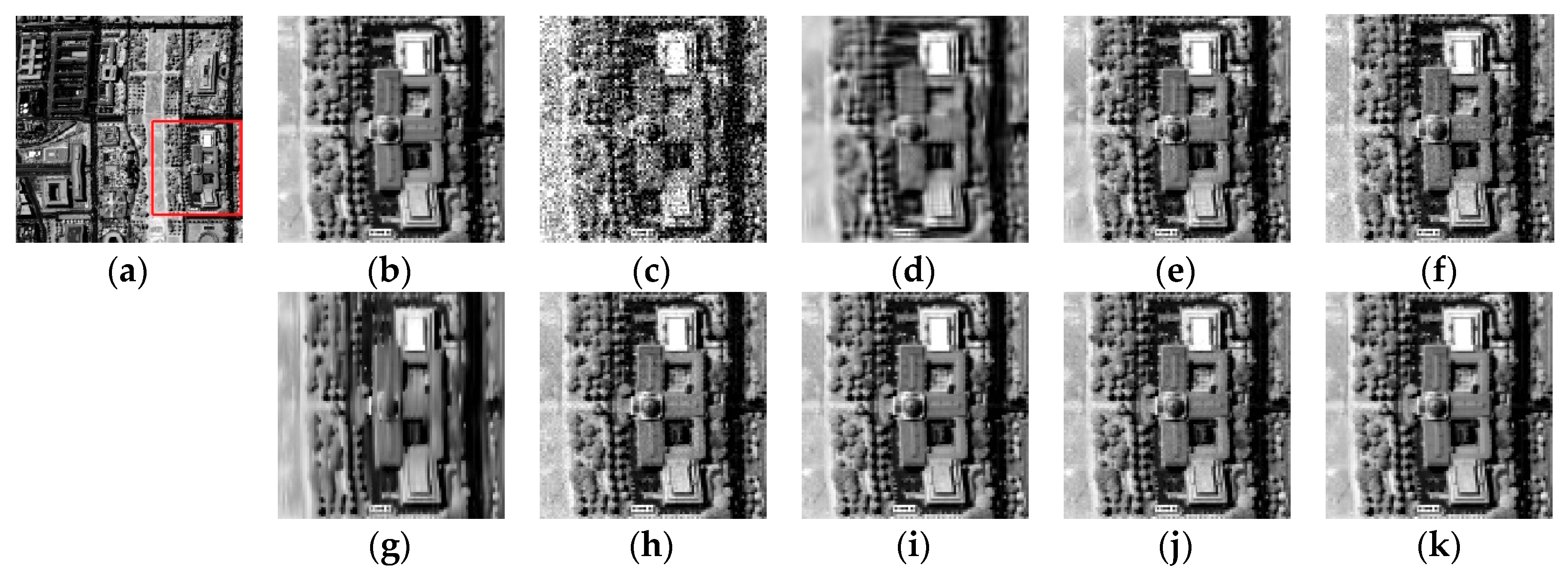
Figure 2, Figure 3 and Figure 4 present the denoising results from different denoising methods with different kinds of noise. Under the Poissonian noise assumption, the Poissonian noise is first transformed into approximate additive Gaussian noise with roughly equal variance by the Anscombe transform [32], and then denoising processing is performed. From the figures, we qualitatively find that the performance of the proposed HyDeSpDLS is better than that of the other denoising algorithms. It can be concluded that all the algorithms are able to denoise the image under all the noise conditions. BM3D, BM4D, and KSVD smooth the details of the denoising results to varying degrees. From Figure 2d,e,g, Figure 3d,e,g and Figure 4d,e,g, we can find that the details of the buildings and green belts are smoothed and blurred. In contrast, PCA + BM4D, LRMR, NAILRMA, and BPFA are better able to preserve local details, as shown in Figure 2f,h–j, Figure 3f,h–j and Figure 4f,h–j. However, these four approaches still leave small amounts of noise in the denoising results. From Figure 2, Figure 3 and Figure 4k, we can find that the proposed HyDeSpDLS is best able to significantly preserve the intrinsic details of the spatial structure when removing the noise.

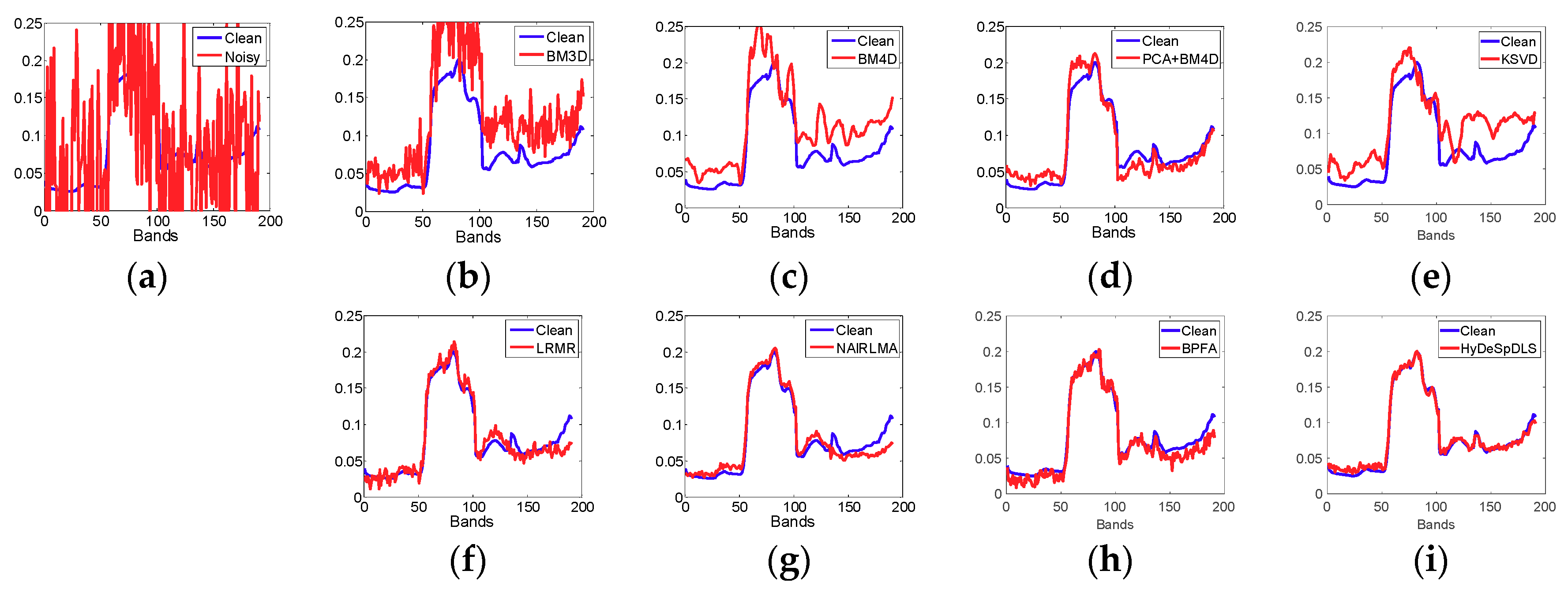
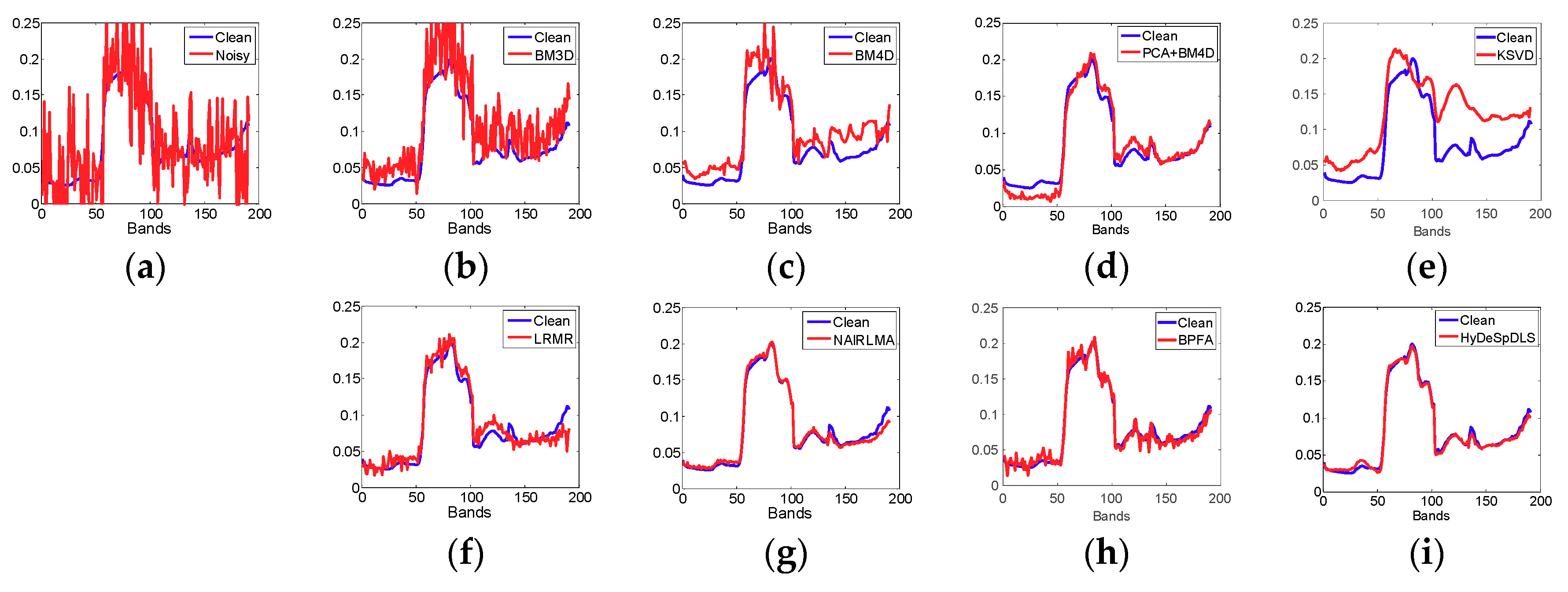
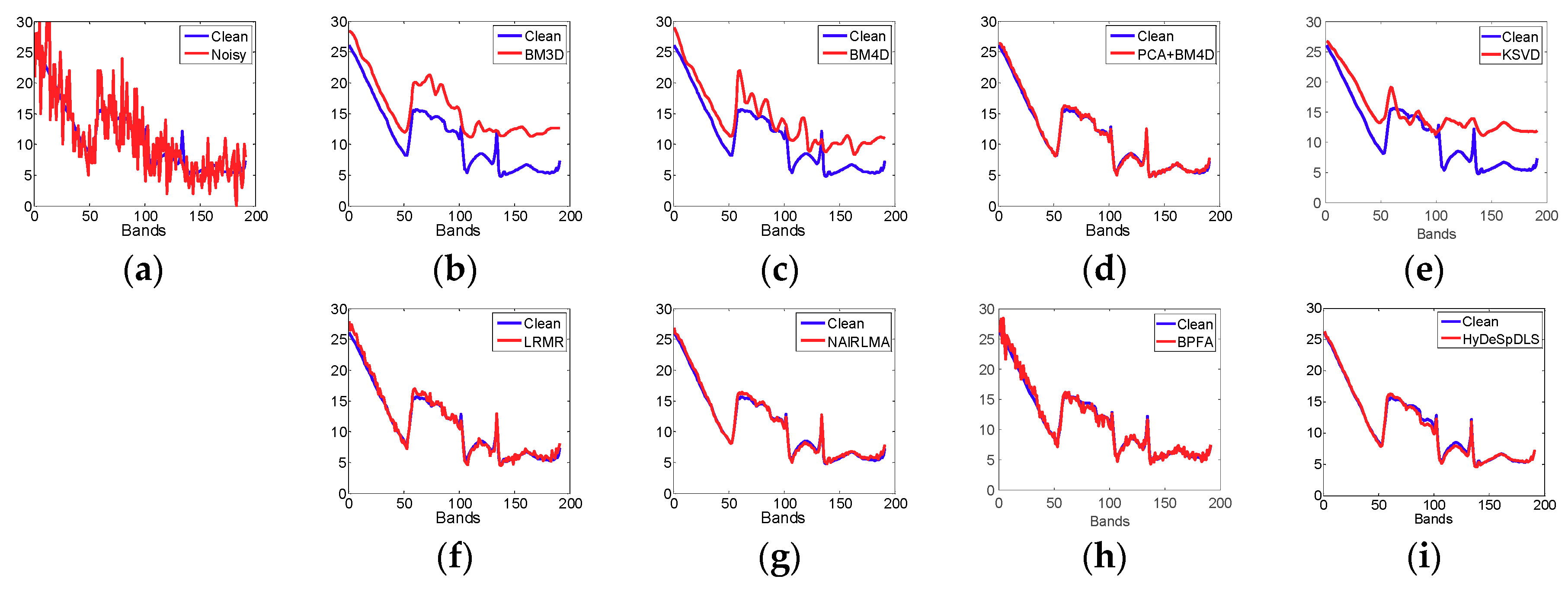
Figure 5, Figure 6 and Figure 7 present the denoised spectral signature results produced by different denoising methods and with different kinds of noise. The quality of the spectral signatures in HSIs is important for material recognition. Due to inadequate use of the spectral information in noisy HSIs, the reconstructed spectra obtained by BM3D, BM4D, and KSVD are quite low, as shown in Figure 5, Figure 6 and Figure 7b,c,e. Considering the low rank property of HSIs, the accuracy of reconstructed spectra obtained by PCA + BM4D, LRMR, NAILRMA, and BPFA improved, as shown in Figure 5, Figure 6 and Figure 7d,f–h. Since the proposed HyDeSpDLS uses a spectral dictionary in which atoms better reflect the details of spectral features in the noisy HSI, this algorithm yields the best performance in restoring the spectral signatures, as shown in Figure 5, Figure 6 and Figure 7i.

Table 1. Quantitative indexes of different denoising algorithms applied to the Washington DC Mall image.

	$\mathit{\sigma }$	Index	Noisy Image	BM3D	BM4D	PCA + BM4D	KSVD	LRMR	NAILRMA	BPFA	HyDeSpDLS
Gaussian i.i.d noise	0.04	MPSNR(dB)	27.9599	32.0285	38.9044	43.3227	37.8230	40.9294	43.1509	43.3978 1	44.47892
		MSSIM	0.8102	0.9164	0.981	0.9917	0.9741	0.9887	0.9920	0.9925	0.9940
	0.06	MPSNR(dB)	24.4361	29.8152	36.2168	39.9911	34.8703	37.7729	40.2376	40.5005	41.7362
		MSSIM	0.6825	0.8668	0.9652	0.9824	0.9496	0.9775	0.9848	0.9860	0.9893
	0.08	MPSNR(dB)	21.9372	28.3672	34.3281	37.9954	32.7267	35.5986	38.1823	38.5642	39.8037
		MSSIM	0.5731	0.8207	0.9473	0.9754	0.9193	0.9641	0.9766	0.9788	0.9851
	0.10	MPSNR(dB)	20.00	27.3065	32.9145	35.6893	31.0701	34.0465	36.6888	37.0405	38.3517
		MSSIM	0.4832	0.7786	0.9281	0.9555	0.8861	0.9504	0.9687	0.9783	0.9791
	0.12	MPSNR(dB)	18.4155	26.4758	31.7905	34.1409	29.7226	32.8334	35.3872	35.7854	37.0672
		MSSIM	0.4100	0.7400	0.9087	0.9388	0.8515	0.9361	0.9597	0.9619	0.9735
Gaussian non-i.i.d noise		MPSNR(dB)	28.6158	32.9923	35.9756	37.0414	28.2282	37.7938	44.5577	44.5680	51.3974
		MSSIM	0.7507	0.8928	0.9616	0.9330	0.7928	0.9754	0.9945	0.9914	0.9985
Poissonian noise		MPSNR(dB)	26.9804	31.2915	38.8223	39.5616	30.7916	40.2634	42.1077	39.7885	42.7277
		MSSIM	0.8003	0.9118	0.9814	0.9804	0.8658	0.9843	0.9888	0.9792	0.9913

¹ The second highest value in each row is underlined. ² The highest value in each row is shown in bold.

shows the mean SSIMs (MSSIM) and the mean PSNRs (MPSNR) in the Washington DC Mall data. The highest values are shown in bold and the second highest values are underlined. It can be concluded from Table 1 that the performance of the proposed HyDeSpDLS is the best in both indexes under all the noise conditions. With increasing noise, the improvements produced by HyDeSpDLS also increase, compared with other denoisers. Compared with the dictionary learning-based denoisers, namely BPFA and KSVD, the denoising performance of the proposed HyDeSpDLS is significantly better.

The running times of different denoising algorithms are shown in

Table 2. Computational time (seconds) of different denoising algorithms applied to the Washington DC Mall image.

	BM3D	BM4D	PCA + BM4D	KSVD	LRMR	NAILRMA	BPFA	HyDeSpDLS
Gaussian i.i.d. noise	169	1024	985	3536	135	158	4315	566
Gaussian non-i.i.d. noise	144	1028	997	3492	127	359	29907	564
Poissonian noise	156	1102	1008	3808	128	96	26904	516

. We can find that, compared with the dictionary-learning-based denoisers, namely BPFA and KSVD, the running time of the proposed HyDeSpDLS is much shorter. It can be concluded that the dictionary learning method applied in HyDeSpDLS has less computational complexity. However, the proposed HyDeSpDLS needs more time than low-rank based algorithms, namely LRMR and NAILRMA, and it may be improved in future research.

5.2. Real-World Data

5.2.1. Data Description

HyDeSpDLS is applied to the Indian Pine data acquired by the AVIRIS (airborne visible/infrared imaging spectrometer) hyperspectral sensor over Northwestern Indiana, USA in June 1992. There are 145 × 145 pixels in the image, with a spatial resolution of 20 m per pixel, and 220 bands with atmospheric correction. It is assumed that the noise in the dataset is non-i.i.d and displays a strong effect in a number of bands.

5.2.2. Experimental Results

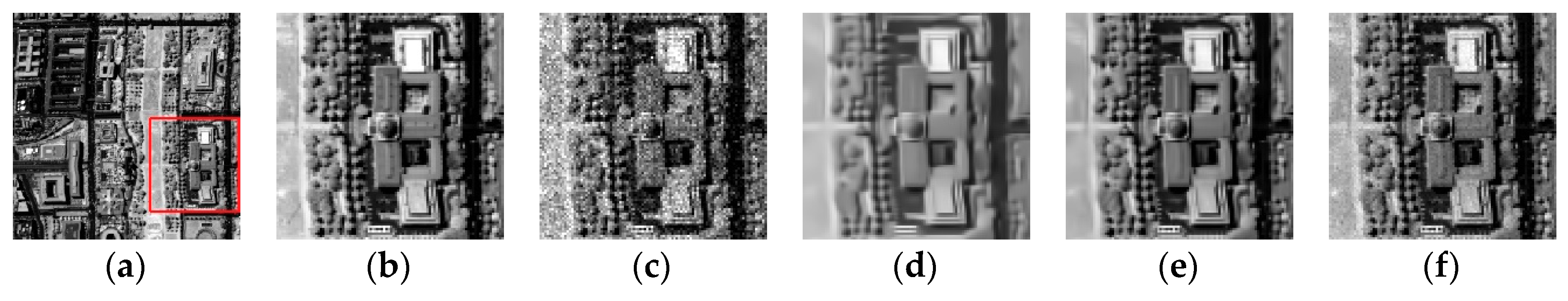
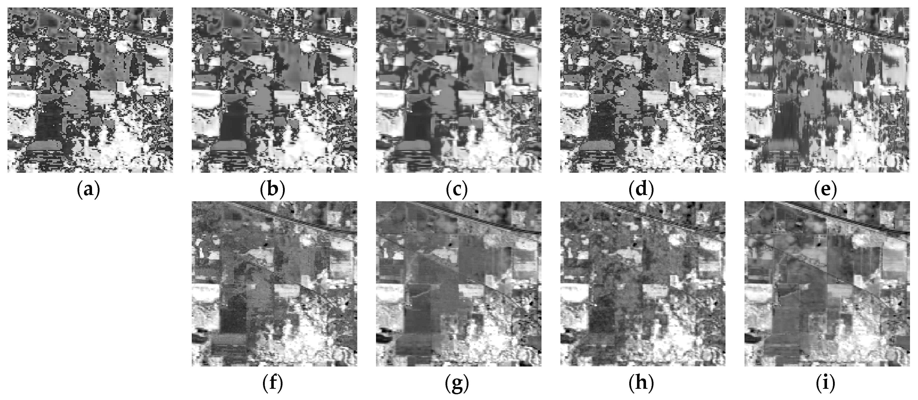
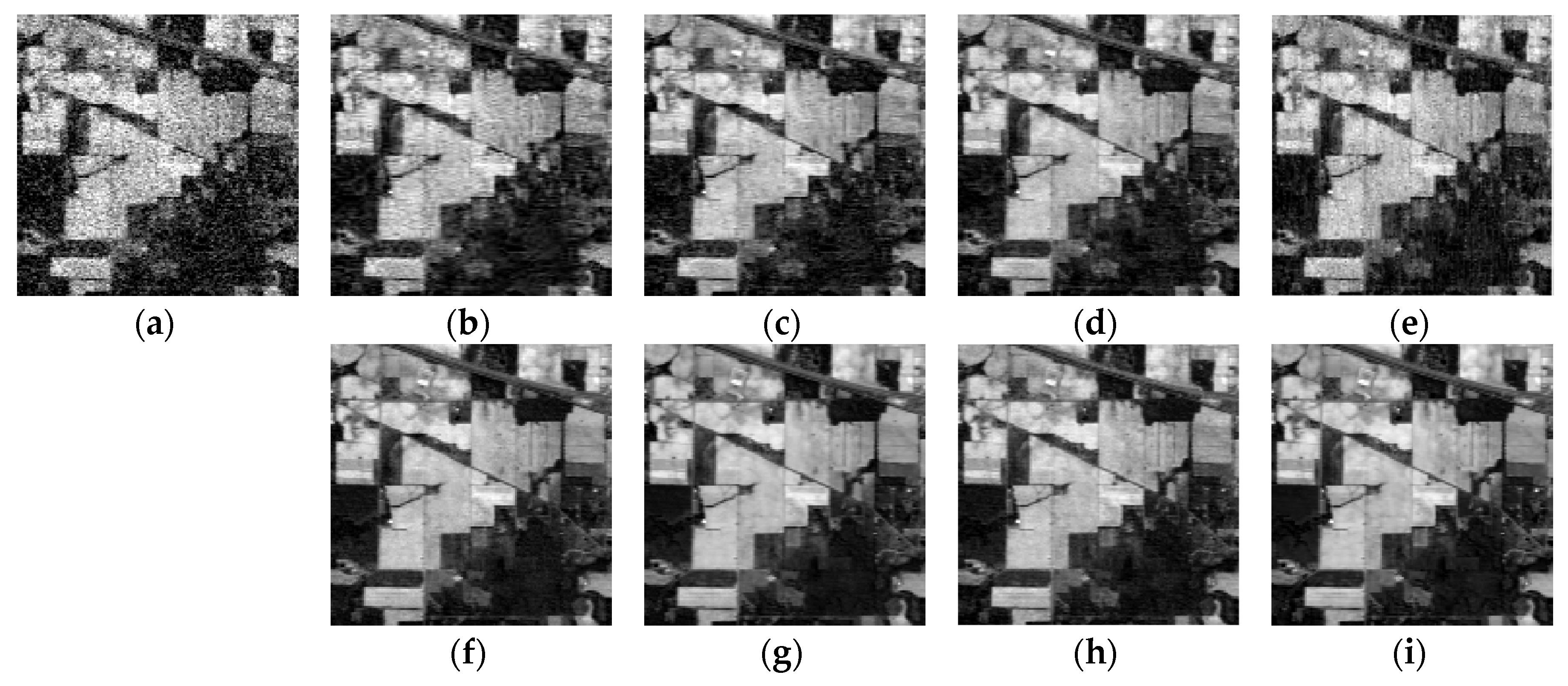
Since there are mass bands in the dataset, only the 61st and 110th bands are selected to illustrate the denoising performance of different algorithms. The image displays strong noise and high brightness in the 61st band, as shown in Figure 8a. Qualitatively, the proposed HyDeSpDLS produces the best denoising result and the spatial structure details, such as edges of the image, are well preserved. In contrast, the image displays weak noise and low brightness in the 110th band, as shown in Figure 9a. BM3D, BM4D, and KSVD can more or less remove the noise, as shown in Figure 9b,c,e, respectively. PCA + BM4D, LRMR, and BPFA remove the noise moderately, as presented in Figure 9d,f,h, respectively. However, the three approaches also smooth the details. NAILRMA and the proposed HyDeSpDLS produce the best denoising results and HyDeSpDLS better preserves the details of spatial structures compared to NAILRMA, as shown in Figure 9g,i, respectively. This further illustrates the robustness of the proposed method with different noise intensities and image brightness.

6. Conclusions

In this paper, a novel denoising method for HSI, called HyDeSpDLS, is proposed based on dictionary learning and sparse coding and extended to the spectral domain. Firstly, the noisy HSI data cube is expanded into a pixel spectral matrix by the scan lines first. A training set consisting of pixel spectral vectors from the matrix is used to train the spectral dictionary for image sparse representation. The spatial-contextual information present in the noisy HSI is exploited as a priori knowledge when completing the sparse coding. Compared with the existing algorithms, including BPFA, NAILRMA, PCA+BM4D, BM4D, BM3D, KSVD, and LRMR, the performance of the proposed method is much better. The intrinsic details of both spatial and spectral structures are well preserved with significant denoising, according to qualitative observations and quantitative indexes. However, the proposed algorithm still has a time consumption problem. In future research, we will focus on a faster implementation of the algorithm.

References

- Zhong, P.; Wang, R. Multiple-spectral-band CRFs for denoising junk bands of hyperspectral imagery. IEEE Trans. Geosci. Remote Sens. 2013, 51, 2260–2275. [Google Scholar] [CrossRef]
- Qian, Y.; Ye, M. Hyperspectral imagery restoration using nonlocal spectral-spatial structured sparse representation with noise estimation. IEEE J. Sel. Top. Appl. Earth Obs. Remote Sens. 2013, 6, 499–515. [Google Scholar] [CrossRef]
- Bioucas-Dias, J.M.; Plaza, A.; Dobigeon, N.; Parente, M.; Du, Q.; Gader, P.; Chanussot, J. Hyperspectral unmixing overview: Geometrical, statistical, and sparse regression-based approaches. IEEE J. Sel. Top. Appl. Earth Obs. Remote Sens. 2012, 5, 354–379. [Google Scholar] [CrossRef]
- Xu, X.; Shi, Z.; Pan, B. ℓ0-based sparse hyperspectral unmixing using spectral information and a multi-objectives formulation. ISPRS J. Photogramm. Remote Sens. 2018, 141, 46–58. [Google Scholar] [CrossRef]
- Li, J.; Zhang, H.; Huang, Y.; Zhang, L. Hyperspectral image classification by nonlocal joint collaborative representation with a locally adaptive dictionary. IEEE Trans. Geosci. Remote Sens. 2014, 52, 3707–3719. [Google Scholar] [CrossRef]
- Pan, B.; Shi, Z.; Xu, X. MugNet: Deep learning for hyperspectral image classification using limited samples. ISPRS J. Photogramm. Remote Sens. 2018, 145, 108–119. [Google Scholar] [CrossRef]
- Stein, D.W.J.; Beaven, S.G.; Hoff, L.E.; Winter, E.M.; Schaum, A.P.; Stocker, A.D. Anomaly detection from hyperspectral imagery. IEEE Signal Process. Mag. 2002, 19, 58–69. [Google Scholar] [CrossRef] [Green Version]
- Zhang, L.; Zhang, L.; Tao, D.; Huang, X. Sparse transfer manifold embedding for hyperspectral target detection. IEEE Trans. Geosci. Remote Sens. 2014, 52, 1030–1043. [Google Scholar] [CrossRef]
- He, W.; Zhang, H.; Shen, H.; Zhang, L. Hyperspectral image denoising using local low-rank matrix recovery and global spatial–spectral total variation. IEEE J. Sel. Top. Appl. Earth Obs. Remote Sens. 2018, 11, 713–729. [Google Scholar] [CrossRef]
- Ghamisi, P.; Yokoya, N.; Li, J.; Liao, W.; Liu, S.; Plaza, J.; Rasti, B.; Plaza, A. Advances in hyperspectral image and signal processing: A comprehensive overview of the state of the art. IEEE Geosci. Remote Sen. Mag. 2018, 5, 37–78. [Google Scholar] [CrossRef]
- Dabov, K.; Foi, A.; Katkovnik, V.; Egiazarian, K. Image Denoising by Sparse 3-D Transform-Domain Collaborative Filtering. IEEE Trans. Image Process. 2007, 16, 2080. [Google Scholar] [CrossRef] [PubMed]
- Rudin, L.I.; Osher, S.; Fatemi, E. Nonlinear total variation based noise removal algorithms. Phys. D Nonlinear Phenom. 1992, 60, 259–268. [Google Scholar] [CrossRef]
- Buades, A.; Coll, B.; Morel, J.M. A Non-Local Algorithm for Image Denoising. In Proceedings of the 2005 IEEE Computer Society Conference on Computer Vision and Pattern Recognition, San Diego, CA, USA, 20–25 June 2005; pp. 60–65. [Google Scholar] [CrossRef]
- Dabov, K.; Foi, A.; Egiazarian, K. Video denoising by sparse 3D transform-domain collaborative filtering. In Proceedings of the 2007 European Signal Processing Conference, Poznan, Poland, 3–7 September 2007; pp. 145–149. [Google Scholar]
- Maggioni, M.; Katkovnik, V.; Egiazarian, K.; Foi, A. A Nonlocal transform-domain filter for volumetric data denoising and reconstruction. IEEE Trans. Image Process. 2013, 22, 119–133. [Google Scholar] [CrossRef] [PubMed]
- Chen, G.; Bui, T.D.; Quach, K.G.; Qian, S. Denoising Hyperspectral Imagery Using Principal Component Analysis and Block-Matching 4D Filtering. Can. J. Remote Sens. 2014, 40, 60–66. [Google Scholar] [CrossRef]
- Zhang, H.; He, W.; Zhang, L.; Shen, H. Hyperspectral Image Restoration Using Low-Rank Matrix Recovery. IEEE Trans. Geosci. Remote Sens. 2014, 52, 4729–4743. [Google Scholar] [CrossRef]
- He, W.; Zhang, H.; Zhang, L.; Shen, H.; Yuan, Q. Hyperspectral Image Denoising via Noise-Adjusted Iterative Low-Rank Matrix Approximation. IEEE J. Sel. Top. Appl. Earth Obs. Remote Sens. 2015, 8, 3050–3061. [Google Scholar] [CrossRef]
- Elad, M.; Figueiredo, M.A.T.; Ma, Y. On the Role of Sparse and Redundant Representations in Image Processing. Proc. IEEE 2010, 98, 972–982. [Google Scholar] [CrossRef] [Green Version]
- Mingyuan, Z.; Haojun, C.; John, P.; Ren, L.; Li, L.; Xing, Z.; Dunson, D.; Sapiro, G.; Carin, L. Nonparametric Bayesian dictionary learning for analysis of noisy and incomplete images. IEEE Trans. Image Process. 2012, 21, 130–144. [Google Scholar] [CrossRef]
- Zhuang, L.; Bioucas-Dias, J.M. Fast Hyperspectral Image Denoising and Inpainting Based on Low-Rank and Sparse Representations. IEEE J. Sel. Top. Appl. Earth Obs. Remote Sens. 2018, 11, 730–742. [Google Scholar] [CrossRef]
- Zhang, L.; Li, J. Development and prospect of sparse representation-based hyperspectral image processing and analysis. J. Remote Sens. 2016, 20, 1091–1101. [Google Scholar] [CrossRef]
- Aharon, M.; Elad, M.; Bruckstein, A. K-SVD: An algorithm for designing overcomplete dictionaries for sparse representation. IEEE Trans. Signal Process. 2006, 54, 4311. [Google Scholar] [CrossRef]
- Shen, H.; Li, X.; Zhang, L.; Tao, D.; Zeng, C. Compressed Sensing-Based Inpainting of Aqua Moderate Resolution Imaging Spectroradiometer Band 6 Using Adaptive Spectrum-Weighted Sparse Bayesian Dictionary Learning. IEEE Trans. Geosci. Remote Sens. 2013, 52, 894–906. [Google Scholar] [CrossRef]
- Mairal, J.; Bach, F.; Ponce, J.; Sapiro, G. Online dictionary learning for sparse coding. In Proceedings of the 26th Annual International Conference on Machine Learning, Montreal, QC, Canada, 14–18 June 2009. [Google Scholar]
- Hao, H.; Wu, L.; Huang, W. Denoising of Complex Valued Images by Sparse Representation. J. Comput. Aided Des. Comput. Gr. 2015, 27, 264–270. [Google Scholar]
- Hao, H.; Bioucas-Dias, J.M.; Katkovnik, V. Interferometric Phase Image Estimation via Sparse Coding in the Complex Domain. IEEE Trans. Geosci. Remote Sens. 2015, 53, 2587–2602. [Google Scholar] [CrossRef] [Green Version]
- Song, X.; Wu, L.; Hao, H. Hyperspectral Image Denoising base on Adaptive Sparse Representation. In Proceedings of the IEEE Third International Conference on Data Science in Cyberspace, Guangzhou, China, 18–21 June 2018. [Google Scholar]
- Bioucas-Dias, J.M.; Figueiredo, M.A.T. Alternating Direction Algorithms for Constrained Sparse Regression: Application to Hyperspectral Unmixing. arXiv, 2010; arXiv:1002.4527. [Google Scholar]
- O’Brien, C.M. Statistical Learning with Sparsity: The Lasso and Generalizations; Chapman & Hall/CRC Press: Boca Raton, FL, USA, 2015; pp. 121–122. ISBN 9781498712163. [Google Scholar]
- Iordache, M.D.; Bioucas-Dias, J.M.; Plaza, A. Total Variation Spatial Regularization for Sparse Hyperspectral Unmixing. IEEE Trans. Geosci. Remote Sens. 2012, 50, 4484–4502. [Google Scholar] [CrossRef] [Green Version]
- Makitalo, M.; Foi, A. A Closed-Form Approximation of the Exact Unbiased Inverse of the Anscombe Variance-Stabilizing Transformation. IEEE Trans. Image Process. 2011, 20, 2697–2698. [Google Scholar] [CrossRef]
Figure 1.
The process of the proposed denoising approach. HSI: hyperspectral image. M is the number of samples in a single scan, N is the scan number in the image, L is the band number, and k is the number of atoms in the trained spectral dictionary. The non-zero elements in the matrix are represented by the color blocks. The white blocks represent the zero elements.
Figure 2.
Denoising results for band 60 of Washington DC Mall data with Gaussian i.i.d. noise: (a) Clean image; (b) zoomed area of clean image in red box of (a); (c) noisy image; (d) BM3D; (e) BM4D; (f) PCA + BM4D; (g) KSVD; (h) LRMR; (i) NAILRMA; (j) BPFA; and (k) HyDeSpDLS.
Figure 3.
Denoising results for band 60 of Washington DC Mall data with Gaussian non-i.i.d. noise: (a) Clean image; (b) zoomed area of clean image in red box of (a); (c) noisy image; (d) BM3D; (e) BM4D; (f) PCA + BM4D; (g) KSVD; (h) LRMR; (i) NAILRMA; (j) BPFA; and (k) HyDeSpDLS.
Figure 4.
Denoising results for band 60 of Washington DC Mall data with Poissonian noise: (a) Clean image; (b) zoomed area of clean image in red box of (a); (c) noisy image; (d) BM3D; (e) BM4D; (f) PCA + BM4D; (g) KSVD; (h) LRMR; (i) NAILRMA; (j) BPFA; and (k) HyDeSpDLS.
Figure 5.
Denoised spectral signature results of Washington DC Mall data with Gaussian i.i.d. noise: (a) Noisy; (b) BM3D; (c) BM4D; (d) PCA + BM4D; (e) KSVD; (f) LRMR; (g) NAILRMA; (h) BPFA; and (i) HyDeSpDLS.
Figure 6.
Denoised spectral signature results of Washington DC Mall data with Gaussian non-i.i.d. noise: (a) Noisy; (b) BM3D; (c) BM4D; (d) PCA + BM4D; (e) KSVD; (f) LRMR; (g) NAILRMA; (h) BPFA; and (i) HyDeSpDLS.
Figure 7.
Denoised spectral signature results of Washington DC Mall data with Poissonian noise: (a) Noisy; (b) BM3D; (c) BM4D; (d) PCA + BM4D; (e) KSVD; (f) LRMR; (g) NAILRMA; (h) BPFA; and (i) HyDeSpDLS.
Figure 8.
Denoising results for band 61 of the Indian Pine data: (a) Original image; (b) BM3D; (c) BM4D; (d) PCA + BM4D; (e) KSVD; (f) LRMR; (g) NAILRMA; (h) BPFA; and (i) HyDeSpDLS.
Figure 9.
Denoising results for band 110 of the Indian Pine data: (a) Original image; (b) BM3D; (c) BM4D; (d) PCA + BM4D; (e) KSVD; (f) LRMR; (g) NAILRMA; (h) BPFA; and (i) HyDeSpDLS.