Stock Market Volatility and Trading Volume: A Special Case in Hong Kong With Stock Connect Turnover

Abstract

The cross-boundary Shanghai-Hong Kong and Shenzhen-Hong Kong Stock Connect provides a special data set to study the dynamic relationships among volatility, trading volume and turnover among three stock markets, namely Shanghai, Shenzhen, and Hong Kong. We employ the Granger Causality test with the vector autoregressive model (VAR) to examine whether Stock Connect turnover contributes to future realized volatility and market volume of these three markets. Our results support the evidence of causality from Stock Connect turnover to market volatility and trading volume. The finding of this causality is consistent with the implication of the sequential information arrival model in the literature.

1. Introduction

The Hong Kong Exchanges and Clearing Limited introduced the Shanghai-Hong Kong Stock Connect (SH-HK Stock Connect) on 17 November 2014, and the Shenzheng-Hong Kong Stock Connect (SZ-HK Stock Connect) on 5 December 2016. Stock Connect established investment channels between Mainland China and Hong Kong stock markets for Mainland China, Hong Kong, and overseas investors through mutual order routing connectivity (HKEX 2018). Throughout years of implementation, Stock Connect has been regarded as an opportunity to enhance market liquidity, open A-shares market and accelerate RMB internationalization (HKEX 2018; Wu and Gao 2015). According to HKEX (2018), Mainland China investors can invest in constituent stocks of the Hang Seng Composite Large Cap Index and Hang Seng Composite Mid Cap Index with a daily limit of RMB 42 billion. Meanwhile, Hong Kong investors can invest in constituent A-shares of the Shanghai Stock Exchange (SSE) 180 Index, the SSE 380 Index, the Shenzhen Stock Exchange (SZSE) Component Index and the SZSE Small/Mid-Cap Innovation Index through either the SH-HK Stock Connect Northbound or the SZ-HK Stock Connect Northbound with a daily quota of RMB 52 billion for each connect. In addition, Stock Connect includes stocks listed on both Mainland China and Hong Kong exchanges.

Due to different market structures of Mainland China and Hong Kong, the operations of Northbound trading and Southbound trading are different. Day trading is not permitted for Northbound and stock trading is subjected to a price limit within ±10% while there is no such limitation for Southbound. Short selling, however, is only allowed for Northbound. Moreover, the trading hours of Northbound and Southbound are not aligned. The continuous auction periods of SH-HK Stock Connect Northbound are 09:30–11:30 and 13:00–15:00; SZ-HK Stock Connect Northbound are 09:30–11:30 and 13:00–14:57; SH-HK and SZ-HK Stock Connect Southbound are 09:30–12:00 and 13:00–16:00. Furthermore, individual Mainland China investors are required to hold a balance of no less than RMB 500,000 to be eligible for Southbound trading.

After the launch of SH-HK Stock Connect, eligible Mainland China investors can purchase eligible shares listed on the Stock Exchange of Hong Kong via their own local account. It fosters the integration of Hong Kong and Mainland China stock markets and creates interaction between the two markets in various dimensions. An improved price discovery between the stocks both listed in Hong Kong and Mainland should be expected. Hui and Chan (2018) investigate the impact of stock connect to A-H premium. They show that A-H premium is affected more significantly by the Mainland China market than the Hong Kong market. They conclude that Mainland China market plays a dominant role in the Stock Connect. Burdekin and Siklos (2018) documents that the A-H premium between Hong Kong and Mainland China’s stocks rose substantially from slightly under 100% when the program was launched to nearly 150% in early 2016. In addition to the A-H premium studies, Wang et al. (2017) find significant effects of the Stock Connect on both Shanghai and Shenzhen stock market volatility using daily data, although the impact on the Hong Kong market is minimal. Huo and Ahmed (2017) investigate the impact of the SH-HK Stock Connect and conclude that Stock Connect significantly strengthened volatility spillover between the two markets. However, they find a weak and unstable cointegration relationship after the Connect, while the conditional variance of both stock markets also increased.

Given the existing studies, we investigate the relationship between market returns and trading volume under Stock Connect with unique extra information regarding the volume flows between the two markets. There are two main theories describing the relationship between the stock return and trading volume of the financial market, namely the mixture of distribution hypothesis proposed by Clark (1973) and sequential information arrival hypothesis proposed by Copeland (1976). The mixture of distribution hypothesis originally proposed by Clark (1973) indicates that securities’ return and trading volume follow a joint distribution conditional on the latest information. Changes of assets’ price and trading volume are due to the same underlying information arrival process and hence volume and volatility are correlated. In the sequential information arrival models, Copeland (1976) and later Jennings et al. (1981) hypothesize causal relationship between stock prices and trading volume. This class of models assumes that information is not received simultaneously by all traders. The new information is observed by each market participant sequentially. Once a new flow of information arrives in the market, traders revise their expectations and react accordingly. The lead-lag relationship of the variables arises from the different speed of response upon information arrival.

There is rich literature focusing on the empirical relationship between return volatility and trading volume. Darrat, Rahman and Zhong (2003) examine the contemporaneous correlation as well as the lead-lag relation between trading volume and return volatility in all stocks comprising the Dow Jones industrial average and find significant lead–lag relations between return volatility and trading volume in many the DJIA stocks in accordance with sequential information arrival hypothesis. Lee and Rui (2002) examine the dynamic relationship between stock market trading volume, returns and volatility for both domestic and cross-country markets based on daily data of the three largest stock markets, New York, Tokyo, and London. They use the vector autoregressive (VAR) model to explain the relationship between returns, volume and volatility. Apart from the mentioned researches, the approach of VAR model for investigating the relationship between stock returns, volatility and trading volume was employed by Mestel et al. (2003), Medeiros and Doornik (2006) and Wang (2004). With the existing findings of relationship between trading activity and volatility in both theoretical and empirical aspects, we extend it to the context of the Stock Connect scheme. According to the sequential information arrival hypothesis, the turnovers via Stock Connect should also reflect the view of market participants across Hong Kong, Shanghai, and Shenzhen markets. We then test whether the turnover via Stock Connect provides information about the future market volatility in addition to the trading volume and other market variables.

For the rest of this paper, we first examine the causal relationship among volatility, trading volume and Stock Connect turnover by Granger-causality test and investigate the implication of Stock Connect turnover to future volatility in the framework of VAR model. In Section 2, we provide an overview of our research methods followed by a description of the data set in Section 3 and empirical findings in Section 4. In Section 5, we summarize the results and conclude our findings.

2. Methodology

2.1. Volatility Measure

Chiang et al. (2010) concludes that aggregating intraday squared returns over n continuous short time intervals within the trading day is a natural estimator of the integrated variance, known as the realized variance (RV). Andersen et al. (2003), Barndorff-Nielsen and Shephard (2002), and other researches show that as $n\to \infty$, the realized variance ${\sigma }^2\left(n\right)$ converges to the true daily variance. Thus, the RV can be expressed as:

$${\sigma }^2\left(n\right)=\sum _{k=1}^n{r}_{t+k/n}^2$$

(1)

where n is the number of intervals in a normal trading day. When n is sufficiently large, the measurement errors of true volatility are negligible. Therefore, in this paper, following Andersen et al. (2003), and Chiang et al. (2010), 5-min interval intraday log returns are used for computing daily RV of Shanghai Stock Exchange Composite Index (${\sigma }_{SSE}^2$), Shenzhen Stock Exchange Component Index (${\sigma }_{SZSE}^2$), Hong Kong Hang Seng Index (${\sigma }_{HSI}^2$).

2.2. Classification of Stock Connect Volume

To investigate how Stock Connect relates to China and Hong Kong stock markets, the detrended and normalized market volume and Stock Connect turnover is separated in the following categories shown in

Table 1. Stock Connect Volume Categories (SH-HK and SZ-HK connect).

Variables	Definition
$V_{SSE,t}$	Total volume of Shanghai Stock Exchange Composite Index
$V_{SZSE,t}$	Total volume of Shenzhen Stock Exchange Component Index
$V_{HSI,t}$	Total volume of Hong Kong Hang Seng Index
$n_{SHHK,t}$	Total turnover of Northbound via SH-HK stock connect
$s_{SHHK,t}$	Total turnover of Southbound via SH-HK stock connect
$n_{SZHK,t}$	Total turnover of Northbound via SZ-HK stock connect
$s_{SZHK,t}$	Total turnover of Southbound via SZ-HK stock connect

.

2.3. Vector Autoregressive Framework and Granger Causality Test

Let $y_t$ be the $n\times 1$ vector of endogenous variables. In the context of the application described in the previous section, vector $y_t$ in the models for each market includes the RVs of market index, trading volumes, Stock Connect Northbound and Southbound turnovers as

Table 2. Vectors of endogenous variables in VAR models.

(a) SH-HK Stock Connect
Stock market	Vector of endogenous variables
Hong Kong	$y_t={\left[{\sigma }_{HSI,t}^2{V}_{HSI,t}{n}_t{s}_t\right]}^{\prime }$
Shanghai	$y_t={\left[{\sigma }_{SSE,t}^2{V}_{SSE,t}{n}_t{s}_t\right]}^{\prime }$
(b) SZ-HK Stock Connect
Stock market	Vector of endogenous variables
Hong Kong	$y_t={\left[{\sigma }_{HSI,t}^2{V}_{HSI,t}{n}_t{s}_t\right]}^{\prime }$
Shanghai	$y_t={\left[{\sigma }_{SSE,t}^2{V}_{SSE,t}{n}_t{s}_t\right]}^{\prime }$

Note: $n_t$ and $s_t$ correspond to each Stock Connect.

. For abbreviation, we represent a general form for $y_t$ in each market as $y_t=\left[{\sigma }_t^2{\nu }_t{n}_t{s}_t\right]$.

Based on VAR(p) model framework, we study the interrelationship among Stock Connect turnovers, market volatilities and market volumes. Our empirical study also includes a Granger causality test to examine the relationship between Stock Connect turnover, market volatility and market volume. The results in Section 4 show that Stock Connect turnover provides additional information in predicting future market volatility over trading volume.

Table 2 defines the variable used in VAR models. The upper panel shows the vectors of endogenous variables in VAR models for SH-HK Stock Connect, while the lower panel shows the vectors of endogenous variables in VAR models for Sz-HK Stock Connect.

The Vector Autoregressive (VAR) model is of the general form

$$y_t={\mathsf{\Phi }}_0+{\mathsf{\Phi }}_1{y}_{t-1}+\dots +{\mathsf{\Phi }}_p{y}_{t-p}+u_t,u_t\sim N(0,{\mathsf{\Sigma }}_u)$$

(2)

where $u_t$ is a vector of Gaussian disturbances, ${\mathsf{\Phi }}_0$ is a $n\times 1$ vector and ${\mathsf{\Phi }}_i$ is $n\times n$ matrix for $i=1,\dots ,p$. Or equivalently,

$$\left(\begin{array}{c}{\sigma }_t^2\\ {\nu }_t\\ n_t\\ s_t\end{array}\right)=\left(\begin{array}{c}{\mu }_{\sigma }\\ {\mu }_{\nu }\\ {\mu }_n\\ {\mu }_s\end{array}\right)+\sum _{i=1}^p\left(\begin{array}{cccc}{\varphi }_{\sigma ,i}& {\varphi }_{\nu ,i}& {\varphi }_{n,i}& {\varphi }_{s,i}\\ {\theta }_{\sigma ,i}& {\theta }_{\nu ,i}& {\theta }_{n,i}& {\theta }_{s,i}\\ {\eta }_{\sigma ,i}& {\eta }_{\nu ,i}& {\eta }_{n,i}& {\eta }_{s,i}\\ {\rho }_{\sigma ,i}& {\rho }_{\nu ,i}& {\rho }_{n,i}& {\rho }_{s,i}\end{array}\right)\left(\begin{array}{c}{\sigma }_{t-i}^2\\ {\nu }_{t-i}\\ n_{t-i}\\ s_{t-i}\end{array}\right)+\left(\begin{array}{c}{u}_{\sigma ,t}\\ u_{\nu ,t}\\ u_{n,t}\\ u_{s,t}\end{array}\right)$$

(3)

where ${\sigma }_t^2$ and ${\nu }_t$ denote RV and detrended market trading volume in each market, respectively. Variable $n_t$ and $s_t$ are the different choices of categorized Stock Connect turnover listed in Table 2, and $u_{i,t}$ are the error terms. The optimal lag length p is calculated by using the Bayesian information criterion (BIC) (Schwarz 1978) given by:

$$BIC=-2ln\left(\widehat{L}\right)+kln\left(n\right)$$

(4)

where $\widehat{L}$ denotes maximum log likelihood function value, n denotes the number of observations and k denotes the number of parameters. For Granger causality tests, the first set of null hypotheses is that the detrended Stock Connect volume $n_t$ and $s_t$ do not Granger cause RVs in each market and the second set of null hypotheses is that they do not Granger cause each market volumes. These are equivalent to test the restriction of ${\varphi }_{n,i}={\varphi }_{s,i}=0$ for RVs as well as ${\theta }_{n,i}={\theta }_{s,i}=0$ for market volumes respectively for all $i=1,2,\dots ,n$. The third set of null hypotheses is that market volatility does not Granger cause Northbound and Southbound turnovers, while the fourth set of null hypotheses hypothesis is that the market volumes do not Granger cause Northbound and Southbound turnovers.

3. Data Description

3.1. Data Transformation

We follow Gallant, Rossi and Tauchen (1992) to investigate the trend stationarity of raw trading volume in each market and Stock Connect turnover by volume series regression on a deterministic function of time, namely,

$${\overline{V}}_t=\alpha +{\beta }_{1}t+{\beta }_2{t}^2+{\epsilon }_t$$

(5)

where ${\overline{V}}_t$ denotes raw trading volume in each market and Stock Connect turnover. The detrended volume series is represented by the residuals ${\epsilon }_t$ in the equation.

Table 3. Trend and Unit Root Test of RVs and Trading Volumes.

(a) Panel A: Volume Series Regression
	SSE	SZSE	HSI	SH-HK Northbound	SH-HK Southbound	SZ-HK Northbound	SZ-HK Southbound
$\alpha$	2.064	0.586	1.206	1.499	0.524	0.198	−0.065
	(49.484) **	(19.499) **	(34.047) **	(32.608) **	(10.701) **	(6.175) **	(−1.095)
${\beta }_1$	−4.625 $\times {10}^{-3}$	5.433 $\times {10}^{-3}$	−1.629 $\times {10}^{-3}$	−5.287 $\times {10}^{-3}$	−4.824 $\times {10}^{-4}$	4.249 $\times {10}^{-3}$	7.391 $\times {10}^{-3}$
	(−19.423) **	(13.752) **	(−8.055) **	(−20.143) **	(−1.725)	(10.070) **	(9.526) **
${\beta }_2$	3.70 $\times {10}^{-6}$	−1.31 $\times {10}^{-5}$	2.08 $\times {10}^{-6}$	7.52 $\times {10}^{-6}$	3.08 $\times {10}^{-6}$	1.37 $\times {10}^{-6}$	−5.67 $\times {10}^{-6}$
	(12.981) *	(−12.061) **	(8.576) *	(23.932) *	(9.197) *	(1.181)	(−2.648) **
$R^2$	0.534	0.382	0.085	0.472	0.531	0.854	0.694
(b) Panel B: Unit Root Test
	SSE	SZSE	HSI	SH-HK Northbound	SH-HK Southbound	SZ-HK Northbound	SZ-HK Southbound
RV
$Lags\left(k\right)$	2	2	3
$\tau \left(p\right)$	−6.389 **	−5.235 **	−6.743 **
Detrended volume
$Lags\left(k\right)$	3	5	2	3	3	4	3
$\tau \left(p\right)$	−5.556 **	−4.884 **	−9.460 **	−6.966 **	−5.262 **	−5.064 **	−3.680 **

** Indicates statistical significance at the 0.01 level. * Indicates statistical significance at the 0.05 level.

a reports the coefficients and their t-statistics in parentheses from regressing raw market volumes, and Stock Connect turnovers on time trend variables. Our results show that nonlinear regression models have high $R^2$ values, and the coefficients for both linear and nonlinear time trend variables are significant in general. Therefore, detrending both market volumes and Stock Connect turnovers is essential in our study.

We further test RVs and detrended volumes for unit root by using augmented Dickey-Fuller test (Dickey and Fuller 1979):

$$V_t=\alpha +\rho V_{t-1}+\sum _{i=1}^k{\varphi }_i\mathsf{\Delta }{V}_{t-i}+e_t$$

(6)

where $e_t$ is a residual term following Gaussian distribution. The number of lagged difference terms k is obtained by the Bayesian information criterion (BIC). Table 3b shows that all RVs, detrended volumes, and detrended Stock Connect turnovers are stationary. Hereafter, we use the volume variable as the detrended volume and use the Stock Connect turnover as the detrended Stock Connect turnover.

Table 4. Descriptive statistics for RVs, market volumes, and Stock Connect turnovers. Trend and Unit Root Test of RVs and Trading Volumes.

	SSE	SZSE	HSI	SH-HK Northbound	SH-HK Southbound	SZ-HK Northbound	SZ-HK Southbound
RV:
Mean	2.862 $\times {10}^{-4}$	9.508 $\times {10}^{-5}$	1.175 $\times {10}^{-4}$
Median	7.807 $\times {10}^{-5}$	5.154 $\times {10}^{-5}$	6.724 $\times {10}^{-5}$
Maximum	7.575 $\times {10}^{-3}$	2.073 $\times {10}^{-3}$	1.892 $\times {10}^{-3}$
Minimum	6.614 $\times {10}^{-6}$	1.093 $\times {10}^{-5}$	7.528 $\times {10}^{-6}$
SD	6.328 $\times {10}^{-4}$	1.682 $\times {10}^{-4}$	1.760 $\times {10}^{-4}$
Skewness	5.532	7.032	5.256
Kurtosis	43.524	68.568	39.199
Observation	808	350	808
Raw trading Volume:
Mean	2.536 $\times {10}^{10}$	9.056 $\times {10}^9$	1.945 $\times {10}^9$	5.897 $\times {10}^9$	5.423 $\times {10}^9$	5.321 $\times {10}^9$	3.284 $\times {10}^9$
Median	1.984 $\times {10}^{10}$	8.705 $\times {10}^9$	1.782 $\times {10}^9$	4.855 $\times {10}^9$	4.864 $\times {10}^9$	4.844 $\times {10}^9$	3.001 $\times {10}^9$
Maximum	8.571 $\times {10}^{10}$	1.573 $\times {10}^{10}$	5.702 $\times {10}^9$	2.352 $\times {10}^{10}$	2.536 $\times {10}^{10}$	1.273 $\times {10}^{10}$	1.327 $\times {10}^{10}$
Minimum	7.057 $\times {10}^9$	4.514 $\times {10}^9$	5.260 $\times {10}^8$	6.887 $\times {10}^8$	3.965 $\times {10}^8$	6.746 $\times {10}^8$	3.502 $\times {10}^8$
SD	1.463 $\times {10}^{10}$	2.139 $\times {10}^9$	6.800 $\times {10}^8$	3.523 $\times {10}^9$	3.661 $\times {10}^9$	2.758 $\times {10}^9$	2.164 $\times {10}^9$
Skewness	1.654	0.392	1.851	1.533	1.042	0.364	0.852
Kurtosis	5.171	2.613	8.028	6.046	4.721	2.205	3.936
Observation	808	350	808	808	808	350	350

shows the descriptive statistics of realized volatility, market volume and Stock Connect turnover. The upper part in the table shows that the descriptive statistics of trading volumes, while the lower part in the table shows the descriptive statistics of detrended trading volumes and Stock Connect turnover.

Table 3 shows the summary of trend and unit root test of realized volatilities and trading volumes. Panel A displays the results of regression models of volume series on deterministic function of time such that $V_t=\alpha +{\beta }_{1}t+{\beta }_2{t}^2+{\epsilon }_t$, where $V_t$ denotes the volume in each market and Stock Connect turnovers. Panel B shows the summary of unit root test for volume in each market and Stock Connect turnovers.

3.2. Data Summary

Table 4 shows the summary statistics of market volatilities and raw market volumes of Shanghai Stock Exchange Composite Index (SSE), Shenzhen Stock Exchange Component Index (SZSE) and Hong Kong Hang Seng Index (HSI)as well as Shanghai-Hong Kong (SH-HK) and Shenzhen-Hong Kong (SZ-HK) Stock Connect turnovers. Stock Connect turnover is further divided into Northbound and Southbound volumes. We select the trading days when Shanghai, Shenzhen, and Hong Kong stock markets as well as Northbound and Southbound in Stock Connect are open such that we can compare their inter-relationship. We collect all the data from Bloomberg and Rice Quant.

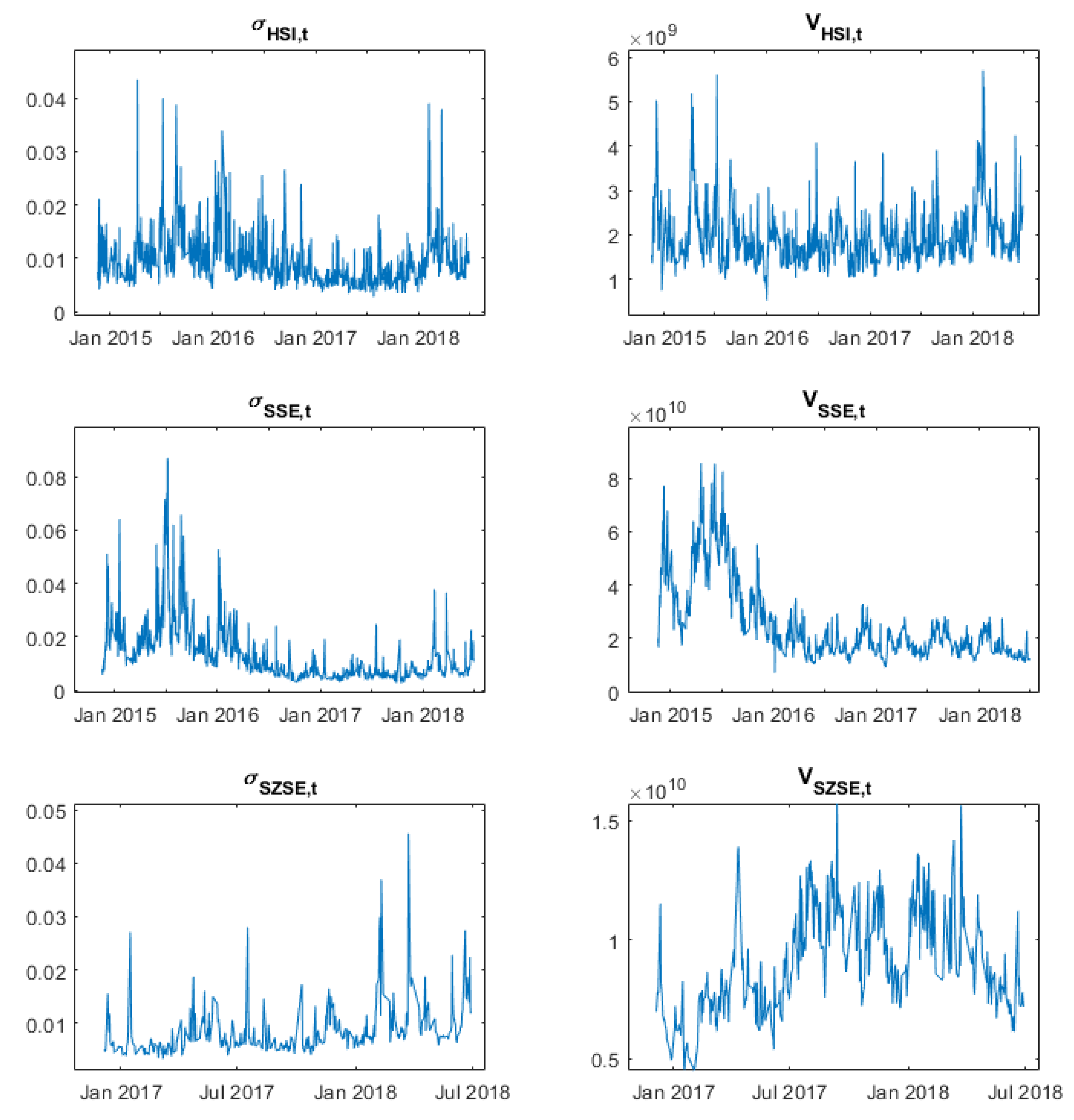
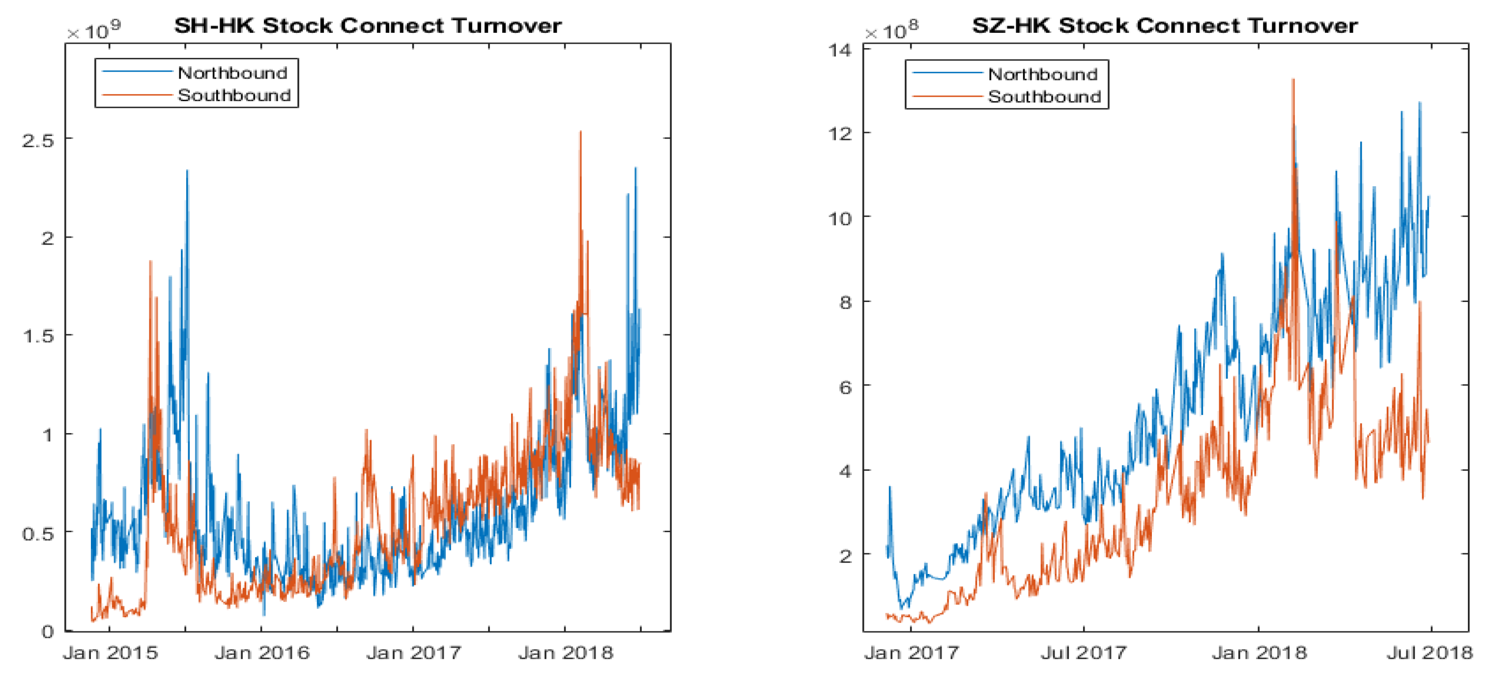
Figure A1 and Figure A2 show the RVs and market volumes of each market as well as Stock Connect turnovers. One can observe that there are co-movement among the variables of Hong Kong, Shanghai, and Shenzhen markets. In particular, RVs and market volumes in SSE and HSI as well as Stock Connect turnovers surged simultaneously in 2015. The trend could be explained by the market boom in early 2015 and sudden market crash during second half of 2015. In 2017, the global market flourished again and yet the China market suffers in 2018. We observe the similar pattern that RVs, market volumes and, Stock Connect turnovers in the three markets surged simultaneously in the short period from 2017 to 2018. Besides, SH-HK and SZ-HK Stock Connect turnovers gradually increase throughout the year. We find that there is a continuous uptrend of Stock Connect turnover and an increasing cointegration of Mainland China and Hong Kong stock market, consistent with Wang and Chong (2018), Wang et al. (2017) and Huo and Ahmed (2017).

Table 5. Stock Connect Correlation Matrix.

(a) SH-HK Stock Connect Correlation Matrix
	${\mathit{\sigma }}_{\mathit{SSE}}^{\mathbf{2}}$	${\mathit{\sigma }}_{\mathit{HSI}}^{\mathbf{2}}$	${\mathit{V}}_{\mathit{SSE}}$	${\mathit{V}}_{\mathit{HSI}}$	$\mathit{n}$	$\mathit{s}$
${\sigma }_{SSE}^2$	1
${\sigma }_{HSI}^2$	0.460	1
$V_{SSE}$	0.528	0.200	1
$V_{HSI}$	0.369	0.514	0.318	1
n	0.326	0.250	0.307	0.548	1
s	−0.170	0.094	−0.159	0.421	0.565	1
(b) SZ-HK Stock Connect Correlation Matrix
	${\mathit{\sigma }}_{\mathit{SZSE}}^{\mathbf{2}}$	${\mathit{\sigma }}_{\mathit{HSI}}^{\mathbf{2}}$	${\mathit{V}}_{\mathit{SZSE}}$	${\mathit{V}}_{\mathit{HSI}}$	$\mathit{n}$	$\mathit{s}$
${\sigma }_{SZSE}^2$	1
${\sigma }_{HSI}^2$	0.749	1
$V_{SZSE}$	0.250	0.250	1
$V_{HSI}$	0.411	0.525	0.305	1
n	0.386	0.382	0.421	0.441	1
s	0.410	0.513	0.491	0.578	0.874	1

a,b shows the correlation matrices ofmarket RVs, market volumes, and all Stock Connect turnovers. We find that Southbound volumes positively correlate with HSI volumes and RVs while Northbound volumes positively correlate with SSE and SZSE market volumes and RVs. This indicates the Stock Connect turnovers have certain degree of dependency to market volatilities and volumes. Moreover, market volumes positively correlate with market volatilities in each market, which is in line with findings of Chen et al. (2001). We also notice that HSI RVs correlate with SSE RVs consistent with Huo and Ahmed (2017). We find similar result for SZSE and HSI RVs in Shenzhen Stock Connect. Also, there is a relatively high correlation between Northbound and Southbound volumes especially in SZ-HK Stock Connect. Although Northbound and Southbound volumes are positively correlated, Northbound volumes appears to be more correlated with RVs and market volumes than Southbound volumes for SH-HK Stock Connect but it is the other way around in SZ-HK Stock Connect. In addition, our results reveal that only SH-HK Southbound turnover negatively correlates with SSE RV and market volume, although the magnitude of negative correlation is not very large. However, there is no such negative correlation among Stock Connect turnover, market volatility and trading volume in SZ-HK Stock Connect.

4. Empirical Findings and Discussion

The Granger causality test results and other details such as the optimal lag lengths in VAR model and Wald statistics are presented in

Table 6. Summary results of Granger causality test.

(a) Panel A: Stock Connect turnover against Market RV and Market Volume
Hypothesis	Comments	Optimal Lag${}^{\mathit{a}}$	Wald Statistics
SH Stock Connect
	SSE
$H_0:{\varphi }_{n,i}={\varphi }_{s,i}=0$, $\forall i$	$n,s\to {\sigma }_{SSE}^2$	2	6.683 (0.035) **
$H_0:{\theta }_{n,i}={\theta }_{s,i}=0$, $\forall i$	$n,s\to {\nu }_{SSE}$	2	9.466 (0.009) ***
	HSI
$H_0:{\varphi }_{n,i}={\varphi }_{s,i}=0$, $\forall i$	$n,s\to {\sigma }_{HSI}^2$	2	27.910 (0.000) ***
$H_0:{\theta }_{n,i}={\theta }_{s,i}=0$, $\forall i$	$n,s\to {\nu }_{HSI}$	2	22.179 (0.000) ***
SZ Stock Connect
	SZSE
$H_0:{\varphi }_{n,i}={\varphi }_{s,i}=0$, $\forall i$	$n,s\to {\sigma }_{SZSE}^2$	1	6.196 (0.013) **
$H_0:{\theta }_{n,i}={\theta }_{s,i}=0$, $\forall i$	$n,s\to {\nu }_{SZSE}$	1	12.775 (0.000) ***
	HSI
$H_0:{\varphi }_{n,i}={\varphi }_{s,i}=0$, $\forall i$	$n,s\to {\sigma }_{HSI}^2$	1	3.110 (0.078) *
$H_0:{\theta }_{n,i}={\theta }_{s,i}=0$, $\forall i$	$n,s\to {\nu }_{HSI}$	1	6.449 (0.011) **
(b) Panel B: Market RV and Market Volume against Stock Connect turnover
Hypothesis	Comments	Optimal Lag${}^{\mathit{a}}$	Wald Statistics
SH Stock Connect
	SSE
$H_0:{\eta }_{\sigma ,1}=0$	${\sigma }_{SSE}^2\to n$	2	2.539 (0.281)
$H_0:{\eta }_{\nu ,1}=0$	${\nu }_{SSE}\to n$	2	5.055 (0.080) *
$H_0:{\rho }_{\sigma ,1}=0$	${\sigma }_{SSE}^2\to s$	2	0.018 (0.991)
$H_0:{\rho }_{\nu ,1}=0$	${\nu }_{SSE}\to s$	2	5.618 (0.060) *
	HSI
$H_0:{\eta }_{\sigma ,1}=0$	${\sigma }_{HSI}^2\to n$	2	0.314 (0.855)
$H_0:{\eta }_{\nu ,1}=0$	${\nu }_{HSI}\to n$	2	5.778 (0.056) *
$H_0:{\rho }_{\sigma ,1}=0$	${\sigma }_{HSI}^2\to s$	2	6.045 (0.049) **
$H_0:{\rho }_{\nu ,1}=0$	${\nu }_{HSI}\to s$	2	0.373 (0.830)
SZ Stock Connect
	SZSE
$H_0:{\eta }_{\sigma ,1}=0$	${\sigma }_{SZSE}^2\to n$	1	0.449 (0.503)
$H_0:{\eta }_{\nu ,1}=0$	${\nu }_{SZSE}\to n$	1	0.425 (0.514)
$H_0:{\rho }_{\sigma ,1}=0$	${\sigma }_{SZSE}^2\to s$	1	6.549 (0.010)**
$H_0:{\rho }_{\nu ,1}=0$	${\nu }_{SZSE}\to s$	1	0.144 (0.704)
	HSI
$H_0:{\eta }_{\sigma ,1}=0$	${\sigma }_{HSI}^2\to n$	1	0.269 (0.604)
$H_0:{\eta }_{\nu ,1}=0$	${\nu }_{HSI}\to n$	1	0.229 (0.632)
$H_0:{\rho }_{\sigma ,1}=0$	${\sigma }_{HSI}^2\to s$	1	1.129 (0.288)
$H_0:{\rho }_{\nu ,1}=0$	${\nu }_{HSI}\to s$	1	0.097 (0.755)

Note: Numbers in parentheses are t-statistics. ^a The optimal lags are chosen with lowest BIC selection criteria. *** Indicates statistical significance at the 0.01 level. ** Indicates statistical significance at the 0.05 level. * Indicates statistical significance at the 0.1 level.

. The overall results indicate that there are unidirectional relationships among Stock Connect turnover, market volatility as well as market volume. Stock Connect turnovers Granger cause RVs and market volumes, but not vice versa.

We first address if the Stock Connect turnovers Granger cause the market volatilities and trading volumes. In the Granger causality test, the null hypotheses that Stock Connect turnovers do not Granger cause market RVs and volumes for SH-HK Stock Connect are both rejected at 1% significant level. Similar results are found in SZ-HK Connect. For SZ-HK Stock Connect, the null hypotheses of no Granger causality from Stock Connect turnovers to market RVs are rejected at 10% significance level, while the null hypotheses of no Granger causality from Stock Connect turnovers to market RVs are rejected at 5% significance level. The Granger causality tests confirm that Turnovers via SH-HK and SZ-HK Stock Connect significantly affect the market volatilities and market turnovers.

However, according to Table 6b, the casual relationship of market RVs and market volumes to Stock Connect turnovers is not as strong as the reverse. About the impact of trading volume, all the null hypotheses of no causality from market volumes to Northbound or Southbound turnovers fail to be rejected at 5% significance level. This indicates that the trading volumes do not contribute directly to Stock Connect turnovers. Higher trading volumes will not influence the activeness of cross-border investors. Similar results are observed from the impact of market volatility. Most of the null hypotheses of no causality from market volatilities to Northbound or Southbound turnovers fail to be rejected at 5% significance level. The only exceptional case is that HSI market volatilities are found to Grange cause Southbound turnovers. The null hypothesis is rejected at 5% level. This may be explained when Hong Kong stock market is more volatile, the capital from Mainland China will be more active to trade. In general, most of the cases are market volatilities or market volumes have no significance impact on either Northbound or Southbound turnovers. Summarizing the results of Granger causality test, the Stock Connect turnovers Granger cause the market volatilities and trading volumes in Both SZ-HK and SH-HK Stock Connect, but not vice versa. Therefore, there are only unidirectional relationships from Stock Connect turnovers to market RVs and market volumes.

Table 7. Summary results of the VAR analysis.

(a) Panel A: Summary results of SH-HK Connect
	RV   ${\mathit{\sigma }}_{\mathit{t}}^{\mathbf{2}}$			Volume  ${\mathit{\nu }}_{\mathit{t}}$			Northbound   ${\mathit{n}}_{\mathit{t}}$			Southbound   ${\mathit{s}}_{\mathit{t}}$
Market	SSE	HSI		SSE	HSI		SSE	HSI		SSE	HSI
${\mu }_{\sigma }$	0.289	0.588	${\mu }_{\nu }$	0.012	0.005	${\mu }_n$	−0.004	0.016	${\mu }_s$	0.001	0.046
	(4.540) ***	(8.870) ***		(0.557)	(0.121)		(−0.138)	(0.490)		(0.045)	(1.699) *
${\varphi }_{\sigma ,1}$	0.430	0.252	${\theta }_{\sigma ,1}$	−0.011	−0.020	${\eta }_{\sigma ,1}$	0.025	−0.001	${\rho }_{\sigma ,1}$	0.000	−0.019
	(11.855) ***	(6.317) ***		(−0.909)	(−0.873)		(1.590)	(−0.039)		(0.038)	(−1.175)
${\varphi }_{\sigma ,2}$	0.282	0.162	${\theta }_{\sigma ,2}$	0.004	0.018	${\eta }_{\sigma ,2}$	−0.016	−0.010	${\rho }_{\sigma ,2}$	−0.002	−0.027
	(7.794) ***	(4.052) ***		(0.327)	(0.787)		(−1.041)	(−0.514)		(−0.127)	(−1.646)
${\varphi }_{\nu ,1}$	0.076	0.045	${\theta }_{\nu ,1}$	0.681	0.467	${\eta }_{\nu ,1}$	0.093	0.012	${\rho }_{\nu ,1}$	−0.029	−0.003
	(0.605)	(0.580)		(16.629) ***	(10.472) ***		(1.735) *	(0.313)		(−0.646)	(−0.086)
${\varphi }_{\nu ,2}$	0.040	−0.036	${\theta }_{\nu ,2}$	0.162	0.077	${\eta }_{\nu ,2}$	−0.026	−0.083	${\rho }_{\nu ,2}$	0.085	0.018
	(0.324)	(−0.475)		(4.006) ***	(1.736) *		(−0.485)	(−2.204) **		(1.915) *	(0.563)
${\varphi }_{n,1}$	0.132	0.089	${\theta }_{n,1}$	−0.033	0.031	${\eta }_{n,1}$	0.484	0.535	${\rho }_{n,1}$	−0.008	−0.001
	(1.324)	(1.126)		(−1.009)	(0.665)		(11.363) ***	(13.832) ***		(−0.215)	(−0.030)
${\varphi }_{n,2}$	0.064	0.131	${\theta }_{n,2}$	0.060	0.050	${\eta }_{n,2}$	0.241	0.270	${\rho }_{n,2}$	0.014	0.053
	(0.642)	(1.652) *		(1.824) *	(1.076)		(5.666) ***	(6.945) ***		(0.385)	(1.642)
${\varphi }_{s,1}$	−0.073	0.325	${\theta }_{s,1}$	0.074	0.061	${\eta }_{s,1}$	0.035	0.035	${\rho }_{s,1}$	0.640	0.643
	(−0.719)	(3.530) ***		(2.210) **	(1.134)		(0.809)	(0.774)		(17.538) ***	(17.053) ***
${\varphi }_{s,2}$	−0.050	−0.353	${\theta }_{s,2}$	−0.035	0.065	${\eta }_{s,2}$	−0.011	0.030	${\rho }_{s,2}$	0.193	0.206
	(−0.486)	(−3.832) ***		(−1.047)	(1.209)		(−0.260)	(0.671)		(5.264) ***	(5.466) ***
$R^2$	0.511	0.191		0.738	0.386		0.563	0.563		0.695	0.695
(b) Panel B: Summary results of SZ-HK Connect
	RV   ${\mathit{\sigma }}_{\mathit{t}}^{\mathbf{2}}$			Volume  ${\mathit{\nu }}_{\mathit{t}}$			Northbound   ${\mathit{n}}_{\mathit{t}}$			Southbound   ${\mathit{s}}_{\mathit{t}}$
Market	SZSE	HSI		SZSE	HSI		SZSE	HSI		SZSE	HSI
${\mu }_{\sigma }$	0.778	0.606	${\mu }_{\nu }$	0.093	0.006	${\mu }_n$	0.017	−0.019	${\mu }_s$	0.062	0.026
	(7.177) ***	(5.774) ***		(1.866) *	(0.118)		(0.313)	(−0.345)		(1.299)	(0.520)
${\varphi }_{\sigma ,1}$	0.224	0.391	${\theta }_{\sigma ,1}$	−0.098	−0.005	${\eta }_{\sigma ,1}$	−0.020	0.017	${\rho }_{\sigma ,1}$	−0.067	−0.030
	(3.795) ***	(6.490) ***		(−3.593) ***	(−0.151)		(−0.670)	(0.518)		(−2.559) **	(−1.063)
${\varphi }_{\nu ,1}$	−0.159	−0.077	${\theta }_{\nu ,1}$	0.632	0.530	${\eta }_{\nu ,1}$	−0.033	0.029	${\rho }_{\nu ,1}$	−0.017	0.017
	(−1.576)	(−0.670)		(13.579) ***	(9.220) ***		(−0.652)	(0.478)		(−0.380)	(0.311)
${\varphi }_{n,1}$	0.058	−0.067	${\theta }_{n,1}$	−0.158	−0.075	${\eta }_{n,1}$	0.452	0.424	${\rho }_{n,1}$	−0.058	−0.094
	(0.511)	(−0.646)		(−3.013) ***	(−1.449)		(7.934) ***	(7.697) ***		(−1.167)	(−1.928) *
${\varphi }_{s,1}$	0.232	0.221	${\theta }_{s,1}$	0.151	0.152	${\eta }_{s,1}$	0.165	0.118	${\rho }_{s,1}$	0.737	0.722
	(2.071) **	(1.756) *		(2.907) ***	(2.409) **		(2.922) ***	(1.765) *		(14.877) ***	(12.197) ***
$R^2$	0.078	0.179		0.383	0.350		0.271	0.270		0.437	0.427

Note: Numbers in parentheses are t-statistics. *** Indicates statistical significance at the 0.01 level. ** Indicates statistical significance at the 0.05 level. * Indicates statistical significance at the 0.1 level.

shows the results for estimated coefficients in the VAR models. The lag lengths of each model, which are chosen with the lowest BIC selection criteria, follow the results in Table 6. Panel A shows the results for SH-HK Stock Connect, while Panel B shows the results for SZ-HK Stock Connect. The table includes estimated coefficients with corresponding t-statistics and adjusted R-square. We find that the coefficients of Stock Connect turnovers in RV and market volume equations are mostly positive. For example, the coefficients of Northbound and Southbound turnover in volatility equation of Shenzhen market are 0.058 and 0.232, respectively. This implies that increase in Stock Connect turnover causes higher market volatility and market volume on the next trading day. In other words, the increase in market volatility follows the rise of activeness of the cross-border investors.

For the market volume equations, we find that the coefficients of Stock Connect turnovers in Shenzhen and Hong Kong market are statistically significant at 5% level mostly, but the coefficients do not have unified sign. For example, the coefficients of northbound and southbound in market volume equation for Shenzhen market are −0.158 and 0.151 respectively, while they are significant at 1% level. Another observation is the negative impacts of the market volatilities on market volume. For example, for SZ-HK Stock Connect, the coefficients of volatility in Shenzhen and Hong Kong market volume equation are −0.098 and −0.005, respectively. It reveals that the relatively low volume follows high market volatility. The results of estimated coefficients in Table 7 are consistent with the results of Granger causality test in which the market RV and market volume do not have significant impact on Northbound and Southbound Volume in general.1

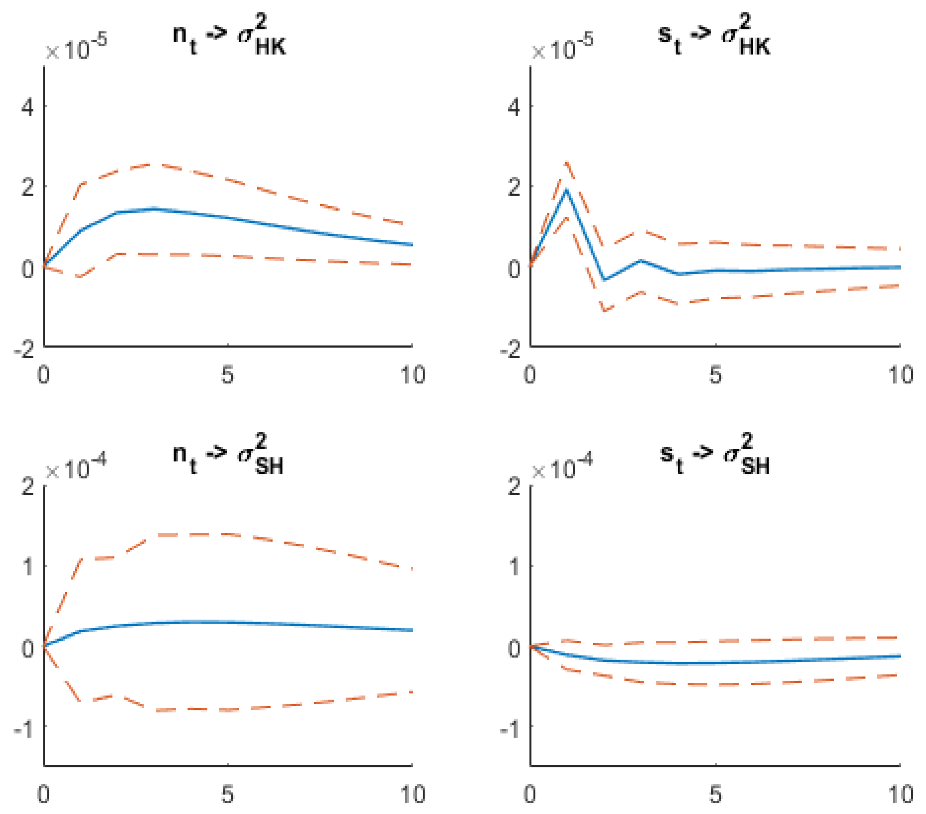
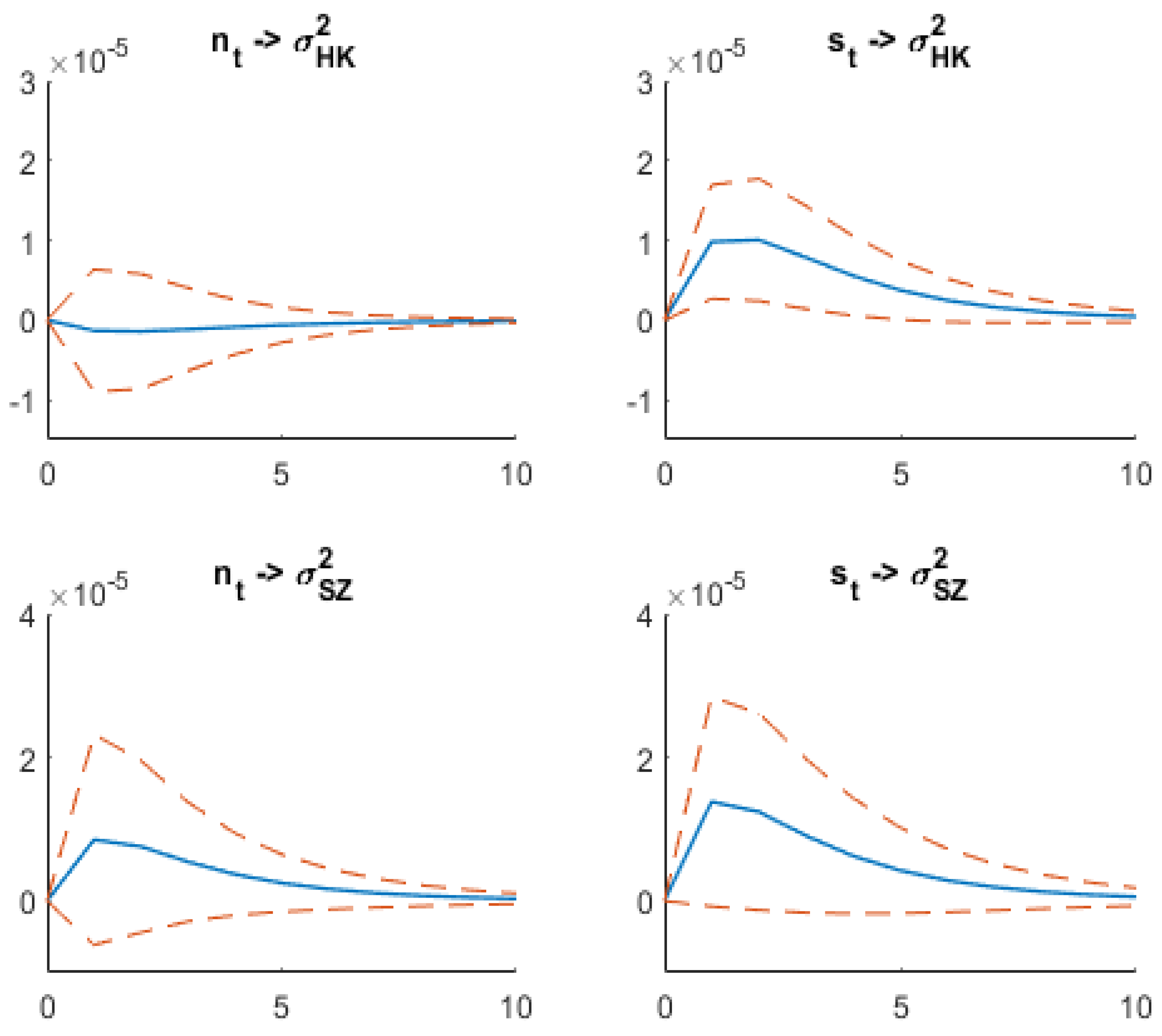
To further investigate the relationship among Stock Connect turnovers, market volatilities and volumes, we examine how the realized volatilities are affected by the shocks of the Stock Connect turnovers via impulse response function 2, as shown in Figure A3 and Figure A4, along with 95% confidence intervals. We consider two groups of impulse responses in turn: realized volatility of Hong Kong and Shanghai indexes response to SH-HK Stock Connect turnover shocks and RVs of Hong Kong and Shenzhen index response to SZ-HK Stock Connect turnover shocks. From Figure A3, we can see that Hong Kong market index has the largest response to the shock of Northbound and Southbound of Stock Connect turnovers in all cases. The Northbound and Southbound turnovers have maximum impacts on Hong Kong market index after 1 day and 4 days, respectively. In SZ-HK Stock Connect, the impact of Stock Connect turnover to Hong Kong market index is higher than that to Shenzhen market index. In general, both Northbound and Southbound Stock Connect turnovers have positive impacts on the realized volatility indexes. The only exceptional case is that Northbound of SZ-HK Connect turnover has a very small negative impact on the volatility of Hong Kong market.

In addition, we perform rolling-window regression to market volatility with the lag term of market volatility, market trading volume and Northbound and Southbound turnovers. To examine the predictive power of Northbound and Southbound of Stock Connect turnovers to the market volatilities, we compare it with the reduced models which omit the lag term of Stock Connect variables. The horizon of rolling-window regression is 250 days. Figure A5 shows the adjusted R-square of the full model minuses that of the reduced model over time. Including Stock Connect turnovers into the regression model gives higher adjusted R-square along time. Higher adjusted R-square of the full model indicates that including the Northbound and Southbound Stock Connect turnovers gives improvements to the predictive models of market volatilities.

5. Conclusions

This paper contributes to the literature of Stock Connect turnover with a focus on the impact of Stock Connect turnovers on volatilities in Shanghai, Shenzhen and Hong Kong stock markets. Our result indicates that there are unidirectional relationships between Stock Connect turnover and market volatility in addition to trading volume. This result clearly suggests the need for a different framework to study realized volatility in stock markets with special features such as the Hong Kong stock market in the future. On the theoretical side, the results are not directly replicable in other markets without the unique trading volume data. On the practical side, our results provide enhanced risk management models for volatility sensitive investment in Hong Kong market.

Table 6 summarizes the results of Granger causality tests. Panel A shows the summary of Granger casualty test of Stock Connect turnover against market RV and market volume, while Panel B shows the summary of Granger casualty test of market RV and market volume against Stock Connect turnover. The first column includes the null hypotheses of the tests and the second column displays the implication of rejecting the null hypotheses. The optimal lag chosen for the test and the Wald statistics with p-values are shown in the third and last columns respectively.

Table 7 displays the estimated parameters and t-statistics of Vector Autoregressive (VAR) models of realized volatilities, market volumes and Northbound and Southbound Stock Connect turnovers. The Vector Autoregressive (VAR) model is of the form

$$\left(\begin{array}{c}{\sigma }_t^2\\ {\nu }_t\\ n_t\\ s_t\end{array}\right)=\left(\begin{array}{c}{\mu }_{\sigma }\\ {\mu }_{\nu }\\ {\mu }_n\\ {\mu }_s\end{array}\right)+\sum _{i=1}^p\left(\begin{array}{cccc}{\varphi }_{\sigma ,i}& {\varphi }_{\nu ,i}& {\varphi }_{n,i}& {\varphi }_{s,i}\\ {\theta }_{\sigma ,i}& {\theta }_{\nu ,i}& {\theta }_{n,i}& {\theta }_{s,i}\\ {\eta }_{\sigma ,i}& {\eta }_{\nu ,i}& {\eta }_{n,i}& {\eta }_{s,i}\\ {\rho }_{\sigma ,i}& {\rho }_{\nu ,i}& {\rho }_{n,i}& {\rho }_{s,i}\end{array}\right)\left(\begin{array}{c}{\sigma }_{t-i}^2\\ {\nu }_{t-i}\\ n_{t-i}\\ s_{t-i}\end{array}\right)+\left(\begin{array}{c}{u}_{\sigma ,t}\\ u_{\nu ,t}\\ u_{n,t}\\ u_{s,t}\end{array}\right)$$

where ${\sigma }_t^2$ and ${\nu }_t$ denote RVs and detrended market trading volumes in each market, respectively. Variable $n_t$ and $s_t$ are the different choices of categorized Stock Connect turnovers, and $u_{i,t}$ are the error terms following Gaussian distribution. The optimal lag length p is calculated by using the Bayesian information criterion (BIC).

References

- Andersen, Torben G., Tim Bollerslev, Francis X. Diebold, and Paul Labys. 2003. Modeling and forecasting realized volatility. Econometrica 71: 579–625. [Google Scholar] [CrossRef]
- Barndorff-Nielsen, Ole E., and Neil Shephard. 2002. Econometric analysis of realized volatility and its use in estimating stochastic volatility models. Journal of the Royal Statistical Society Series B Part 2 64: 253–80. [Google Scholar] [CrossRef]
- Burdekin, Richard C.K., and Pierre L. Siklos. 2018. Quantifying the impact of the November 2014 Shanghai-Hong Kong stock connect. International Review of Economics and Finance 57: 156–163. [Google Scholar] [CrossRef]
- Chen, Gong-meng, Michael Firth, and Oliver M. Rui. 2001. The dynamic relation between stock returns, trading volume, and volatility. Financial Review 36: 153–74. [Google Scholar] [CrossRef]
- Chiang, Thomas C., Zhuo Qiao, and Wing-Keung Wong. 2010. New evidence on the relation between return volatility and trading volume. Journal of Forecasting 29: 502–15. [Google Scholar] [CrossRef]
- Clark, Peter K. 1973. A subordinated stochastic process model with finite variance for speculative prices. Econometrica 41: 135–55. [Google Scholar] [CrossRef]
- Darrat, Ali F., Shafiqur Rahman, and Maosen Zhong. 2003. Intraday trading volume and return volatility of the DJIA stocks. Journal of Banking and Finance 27: 2035–43. [Google Scholar] [CrossRef]
- De Medeiros, Otavio Ribeiro, and Bernardus Ferdinandus Nazar Van Doornik. 2006. The Empirical Relationship Between Stock Returns, Return Volatility and Trading Volume in the Brazilian Stock Market. Available online: https://ssrn.com/abstract=897340 (accessed on 8 August 2018).
- Dickey, David A., and Wayne A. Fuller. 1979. Distribution of the estimators for autoregressive time series with a unit root. Journal of the American Statistical Association 74: 427–31. [Google Scholar] [CrossRef]
- Economics, Thomas E. Copeland. 1976. A model of asset trading under the assumption of sequential information arrival. Journal of Finance 31: 1149–68. [Google Scholar] [CrossRef]
- Gallant, A. Ronald, Peter E. Rossi, and George Tauchen. 1992. Stock prices and volume. The Review of Financial Studies 5: 199–242. [Google Scholar] [CrossRef]
- Hong Kong Exchanges and Clearing Limited. 2008. Stock Connect Another Milestone Information Book for Market Participants. Available online: http://www.hkex.com.hk/-/media/HKEX-Market/Mutual-Market/Stock-Connect/Getting-Started/Information-Booklet-and-FAQ/Information-Book-for-Market-Participants/EP_CP_Book_En_(13July18).pdf (accessed on 8 August 2018).
- Hui, Eddie C.M., and Ka Kwan Kevin Chan. 2018. Does the Shanghai–Hong Kong Stock Connect significantly affect the AH premium of the stocks? Physica A: Statistical Mechanics and its Applications 492: 207–14. [Google Scholar] [CrossRef]
- Huo, Rui, and Abdullahi D. Ahmed. 2017. Return and volatility spillovers effects: Evaluating the impact of Shanghai-Hong Kong Stock Connect. Economic Modelling 61: 260–72. [Google Scholar] [CrossRef]
- Jennings, Robert H., Laura T. Starks, and John C. Fellingham. 1981. An equilibrium model of asset trading with sequential information arrival. Journal of Finance 36: 143–61. [Google Scholar] [CrossRef]
- Lee, Bong-Soo, and Oliver M. Rui. 2002. The dynamic relationship between stock returns and trading volume: Domestic and cross-country evidence. Journal of Banking and Finance 26: 51–78. [Google Scholar] [CrossRef]
- Mestel, Roland, Henryk Gurgul, and Paweł Majdosz. 2003. The Empirical Relationship Between Stock Returns, Return Volatility and Trading Volume on the Austrian Stock Market. Styria, Austria: University of Graz, Institute of Banking and Finance, Research Paper. [Google Scholar]
- Schwarz, Gideon. 1978. Estimating the dimension of a model. The Annals of Statistics 6: 461–64. [Google Scholar] [CrossRef]
- Wang, Hanfeng. 2004. Dynamic Volume-Volatility Relation. Available online: http://ssrn.com/abstract=603841 (accessed on 8 August 2018).[Green Version]
- Wang, Qiyu, and Terence Tai-Leung Chong. 2018. Co-integrated or not? After the Shanghai–Hong Kong and Shenzhen–Hong Kong Stock Connection Schemes. Economics Letters 163: 167–71. [Google Scholar] [CrossRef]
- Wang, Yang-Chao, Jui-Jung Tsai, and Qiaoqiao Li. 2017. Policy impact on the Chinese stock market: From the 1994 bailout policies to the 2015 Shanghai-Hong Kong stock connect. International Journal of Financial Studies 5: 4. [Google Scholar] [CrossRef]
- Wu, Tingting, and Xiaoying Gao. 2015. Factors of Price Difference between A-Shares and H-Shares under SH-HK Stock Connect. In Paper presented at Proceedings of the International Conference on Transnational Corporations and Emerging Markets, Wuhan, October 29–31. [Google Scholar]