Exchange Rate Volatility and Disaggregated Manufacturing Exports: Evidence from an Emerging Country

Abstract

The link between export performance and exchange rate policy has been attracting attention from policymakers, academics, and practitioners for some time, particularly for emerging countries. It has been recently claimed that implementing a policy that devalues the currency in Vietnam is an important factor for enhancing its export performance. However, it is also argued that such a policy could result in the harmful consequence of exchange rate volatility. This study analyzes the link between exchange rate devaluation, volatility, and export performance. The analysis focuses on the manufacturing sector and 10 of its subsectors that were engaged in the export of goods between Vietnam and 26 key export partners during the 2000–2015 period. Potential factors that could affect this relationship, such as the global financial crisis, Vietnam’s participation in the World Trade Organization, or even the export partners’ geographic structures, are also accounted for in the model. The findings confirm that a strategy that depreciates Vietnam’s currency appears to enhance manufacturing exports in the short run, whereas the resulting exchange rate volatility has clear negative effects in the long run. The impact of exchange rate volatility on manufacturing subsectors depends on two factors, namely, (i) the type of export and (ii) the export destination. Policy implications emerging from these conclusions are presented.

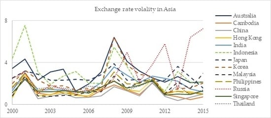
1. Introduction

The impact of exchange rate volatility on exports has generated a great degree of interest among policymakers, economists, and practitioners (exporters and importers in particular). The impact is playing an increasingly important role in many emerging Asian and South American countries, where exports are considered the engine in export-orientated growth models (Kandilov 2008). It is widely believed that an increase in exchange rate volatility could have devastating effects on an economy and its trade, and such outcomes would be the most damaging in emerging nations, where capital markets are likely to be underdeveloped (Prasad et al. 2003). In the context of an emerging market, a comprehensive understanding of the nature and magnitude of the nexus between exchange rate volatility and exports is of great importance to policymakers. Unfortunately, this crucial issue has been largely ignored.

In Vietnam, researchers have examined a variety of factors, such as foreign direct investment (Xuan and Xing 2008), trade policy (Nguyen 2016), and the impact of trade partnerships or agreements (Xiong 2017), that have affected aggregated exports. Nguyen (2016) examined the trade liberalization policy in Vietnam and its link to the level of export sophistication. The study’s findings reveal that trade liberalization has had a stronger effect on the non-manufacturing sector than the manufacturing sector and that being a World Trade Organization (WTO) member does not have any impact on the level of export sophistication in Vietnam. In their analysis, Narayan and Nguyen (2016) used Vietnam as a case study to demonstrate how the variables in the gravity model are dependent on trading partners. Their results indicate that the country’s trading activities are more sensitive to exchanges with rich nations than low-income ones. Also, the issue of Vietnam’s currency depreciation (or devaluation, to use the more accurate term) has been the subject of debate in recent years. Some believe that although this strategy would enhance export performance, it would have the side effect of making exchange rates volatile, which, in turn, may be harmful to exports.

On balance, there are conflicting views in the literature on the relationship between exchange rate volatility and exports: empirical studies have produced mixed results due to differing methodologies, volatility measurements, and the types of data used. To the best of our knowledge, few of these studies have been conducted in the context of Vietnam, so policies may lack evidentiary support from academic studies. Our efforts here are an attempt to fill this gap. This paper aims to provide empirical evidence of the link between exchange rate devaluation, volatility, and export performance in Vietnam at disaggregated levels over a period of 16 years, from 2000 to 2015.

The contributions of this paper are as follows. First, a panel model was used to analyze the relationship between the two main variables of interest—the exchange rate volatility and exports, with a special focus on the manufacturing industry and its 10 subsectors. Details of the 10 subsectors, as well as 26 of Vietnam’s key export partners, are shown in

Table A1. List of Sub-subsector.

Code	OECD	SIC	Sector
EX	D10T32	D10-D32	Manufacturing exports
EX1	D10T12	D10, D11, D12	Food products, beverages and tobacco
EX2	D13T15	D13, D14, D15	Textiles, wearing apparel, leather and related products
EX3	D16	D16	Wood and products of wood and cork, except furniture
EX4	D17T18	D17, D18	Paper and printing
EX5	D19T22	D19, D20, D21, D22	Chemicals, rubber, plastics and fuel products
EX6	D23	D23	Non-metallic mineral products
EX7	D24T25	D24, D25	Basic metals and fabricated metal products, except machinery and equipment
EX8	D26T28	D26, D27, D28	Machinery and equipment
EX9	D29T30	D29, D30	Transport equipment
EX10	D31T32	D31, D32	Furniture and other manufacturing

OECD and SIC represent the classification of the manufacturing export based on the OECD database and Standard Industrial Classification (SIC) Codes, respectively.

and

Table A2. List of Countries.

Regions	Countries
Asia	Australia, Cambodia, Hong Kong, China, India, Indonesia, Japan, Korea, Malaysia, Philippines, Russian, Singapore, Thailand
Europe	Belgium, France, Germany, Italy, Netherlands, Spain, Turkey, United Kingdom
America	Brazil, Canada, Mexico, South Africa, United States

in the Appendix. These partners make up a significant share of Vietnam’s export transactions compared with the rest of the world, and the manufacturing sector plays a substantial role in Vietnam’s export structure. We argue that, in recent years, Vietnam has become a preferred destination for supply chain production for many multinational corporations (MNCs) due to the rise of China (Hooy et al. 2015). Also, the country has become deeply involved in further international economic integration by joining multilateral free-trade agreements, such as the Regional Comprehensive Economic Partnership (RCEP). Second, we reexamined the effect of exchange rate volatility on exports in three different regions (Asia, Europe, and America). We are of the view that the manufacturing exports between Vietnam and its partners in different regions may be influenced by regional factors such as geographic distances, political and economic relationships, and others. This may alter the export structure and the target destination, especially for the manufacturing sector. Therefore, we separated all of the data into three subsamples based on geographical characteristics, which enabled the exploration of whether location contributes to the impact on the nexus between exchange rate volatility and manufacturing exports in Vietnam.

The structure of this paper is as follows. Following this Introduction, information on manufacturing exports and the trend of exchange rate volatility in Vietnam are briefly discussed in Section 2. Section 3 summarizes relevant theories and empirical studies related to exchange rate volatility and exports. Model specifications are presented in Section 4. Section 5 describes the data and presents the empirical results. A concluding remark follows in the remaining section of the paper.

2. Overview of Vietnam’s Exports and Exchange Rate

This section provides some background to provide insight into how the exchange rate market in Vietnam operates, as well as the state of manufacturing exports in Vietnam during the 2000–2015 period. In Vietnam, the exchange rate market is controlled by the State Bank of Vietnam (SBV). In early 1999, it was announced that the exchange rate system would follow a managed floating regime, in which the SBV would publish a daily interbank exchange rate, the average of the exchange rate based on the previous day, and a fluctuation band. The SBV predetermines the fluctuation band for exchange rates to adjust to the market forces of demand and supply, and market participants are expected to trade within the setting band.

Table 1. Fluctuation Bands of USD/VND Exchange Rate, 1999–2015.

Time	Feb.-1999	Jun.-2002	Jan.-2007	Dec.-2007	Mar.-2008	Jun.-2008	Nov.-2008	Mar.-2009	Nov.-2009	Feb.-2011	Aug.-2015
Bands (%)	+ 0.1	+/− 0.25	+/− 0.5	+/− 0.75	+/− 1	+/− 2	+/− 3	+/− 5	+/− 3	+/− 1	+/− 3

provides a summary of fluctuation bands specified by the SBV from 1999 to 2015. Before 2007, the setting bands of VND/USD fluctuated within a narrow range of around 1%. During the 2008 global financial crisis, the SBV allowed the band to widen to 5%, relative to the official quotation, before narrowing it down to 1% in 2011. This band was stable until late 2015, when it increased by 2%. However, according to the exchange rate regime classification by Ilzetzki et al. (2017), Vietnam was classified as a “dual market in which parallel market data is missing” prior to 2002, but the country was set to follow a crawling peg until 2016.

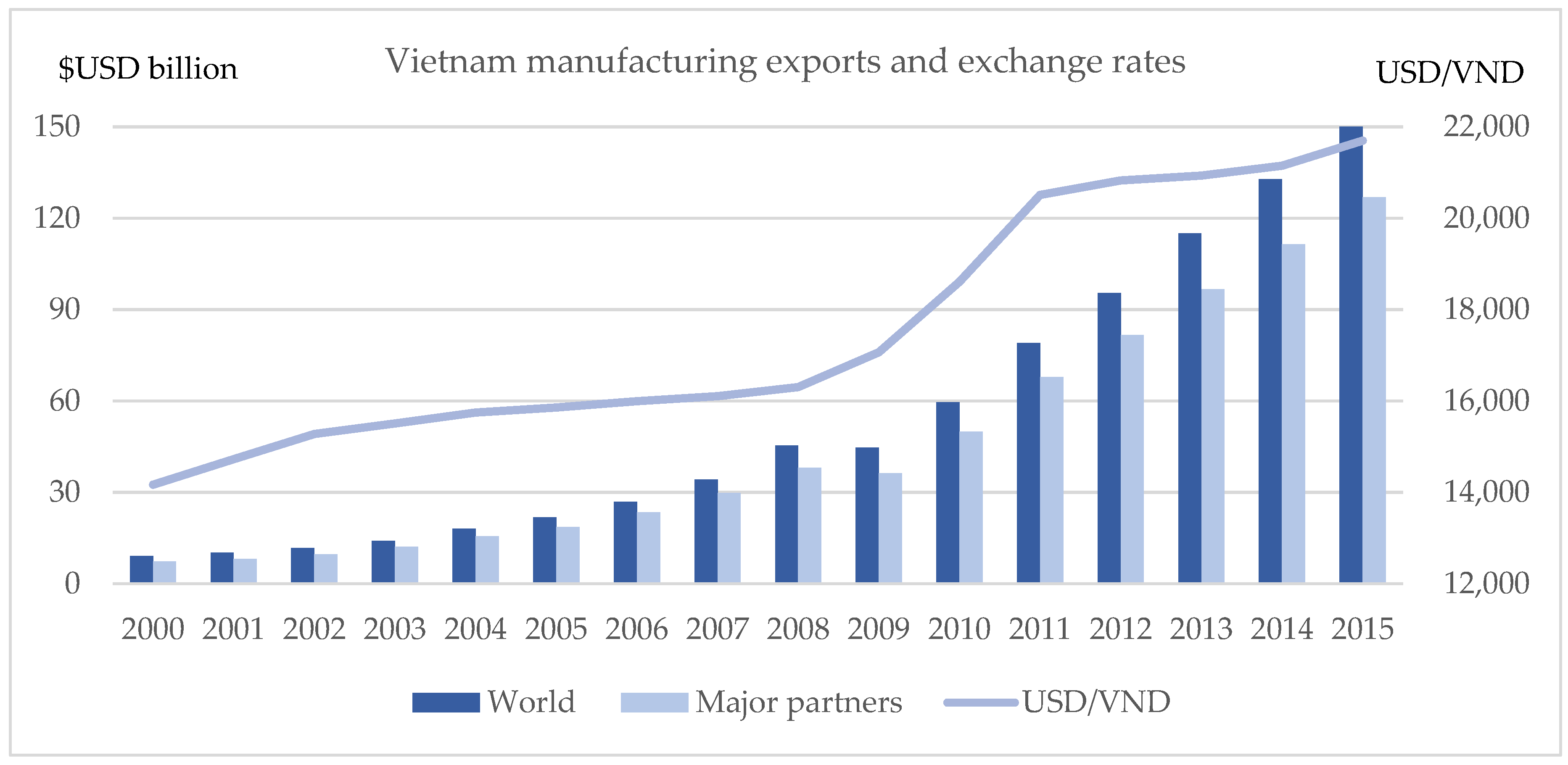
Figure 1 presents the annual values of Vietnam’s manufacturing exports, and the line depicts the trend in the VND/USD exchange rate from 2000 to 2015. There was an upward trend over the timeframe considered. The total value of manufacturing exports started at around 10 billion USD in 2000, gradually increased to approximately 45 billion USD in 2008, and then had a relatively slight decrease in 2009 because of the global financial crisis. After that, the increase was even more significant during the 2009–2015 period, ending up at over 150 billion USD in 2015. A similar trend was seen in the export pattern of 26 other major countries. Regarding the exchange rates, the line graph shows an upward trend from around 14,000 VND per 1 USD in 2000 to approximately 22,000 VND per 1 USD in 2015, indicating a depreciation in VND of more than 120% over the selected period. The most striking detail is that, after the global financial crisis, the exchange rate depreciated dramatically, with a depreciation of around 30% over a period of three years.

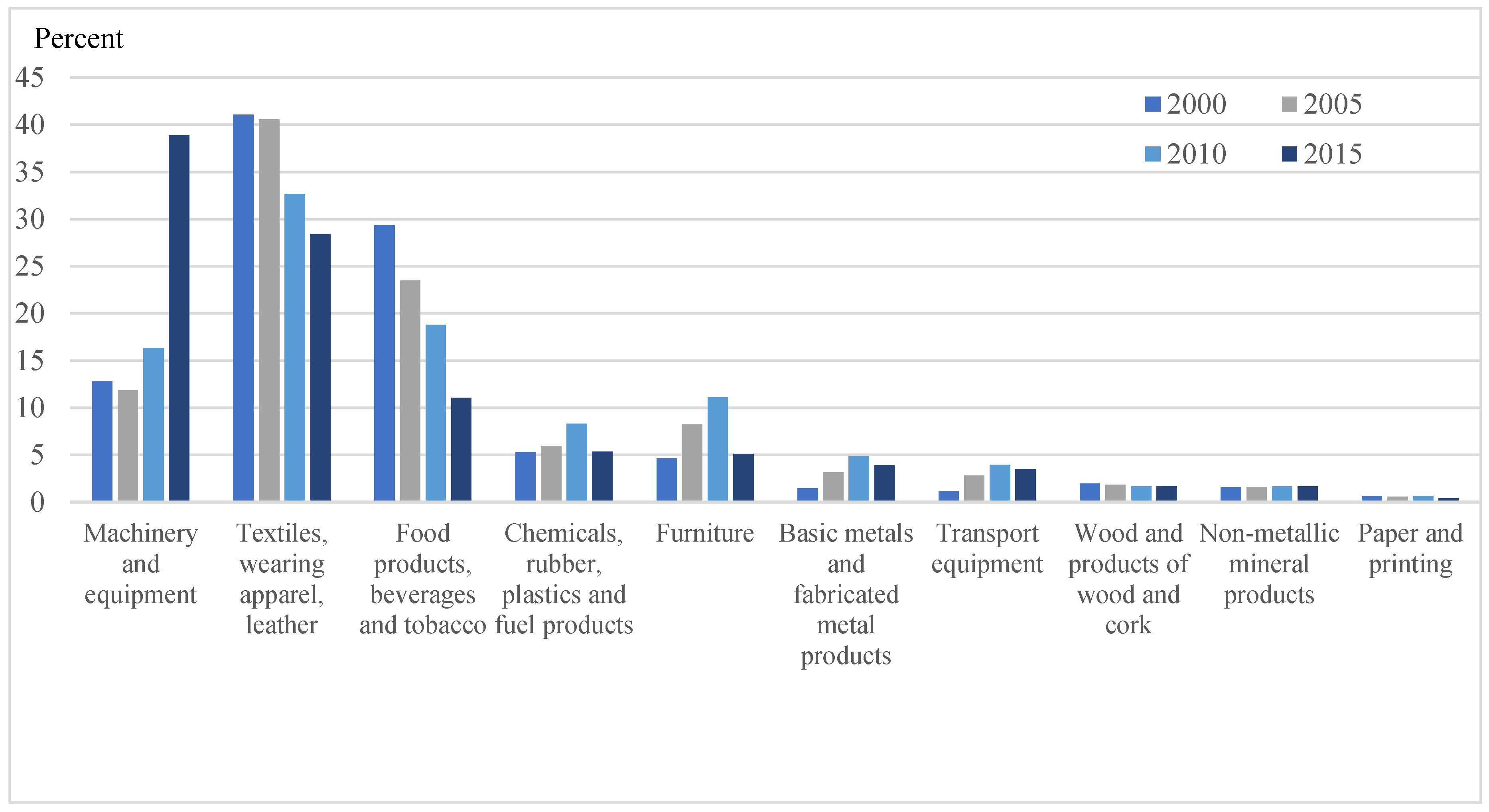
A closer look at Vietnam’s manufacturing sectors is illustrated in Figure 2, which shows the percentage of export value from each subsector of the manufacturing sector in four different years during the period from 2000 to 2015. Importantly, these proportions changed significantly over the period surveyed. In 2000, the largest subsector contributing to overall manufacturing exports was Textiles, wearing apparel, leather, making up more than two-fifths. This was followed by Food products, beverages, and tobacco, which accounted for nearly one-third of the total of manufacturing exports. Textiles continued to account for the majority of exports until 2010. In 2015, Machinery and equipment became the most significant contributor after experiencing a considerable rise from nearly 13% in 2000 to just under two-fifths in 2015. Chemicals, rubber, plastics, and fuel products and Furniture, other manufacturing products were large contributors to the country’s manufacturing exports from 2000 to 2010, but their share declined marginally in 2015. Other industries made up a minuscule part of the total value of manufacturing exports throughout the period of interest.

Based on the above statistics, some observations can be summarized. First, the manufacturing sector is playing an increasingly important role in Vietnam’s exports with regard to the monetary value and the share of total exports, but there has been significant variation in its structure, and it is now dominated by machinery and equipment products. Second, the VND depreciated and fluctuated over the study period, potentially generating detrimental effects on exports, especially in the manufacturing sector.

3. Literature Review

The exchange rate is a key factor that influences the volume and values of exports. Researchers have examined the effect of exchange rates on exports. For example, Hooy et al. (2015) investigated the effect of the Renminbi real exchange rates on ASEAN exports to China. Although the real exchange rate was found to be positively related to ASEAN exports, its effect on disaggregated levels was mixed. The depreciation of the Renminbi real exchange rate had a positive impact on the export of high- and medium-tech finished goods, as well as parts and components, but it had no effect on basic goods or low-tech, resource-based, and primary products. Recently, in a study by Atif et al. (2017), the exchange rate was found to be a stimulating factor of agricultural exports in Pakistan.

Scholars have also assessed the impact of exchange rate changes on exports from a theoretical perspective. On the one hand, the first strand of the theory’s hypothesis is that without a mechanism to mitigate exchange rate risks, volatility will cause a decline in the volume of trade. Exchange rate fluctuations will lead to greater uncertainty in transaction costs, triggering a decrease in the volume of trade (Hooper and Kohlhagen 1978). If traders are uncertain how these fluctuations will influence the company’s revenue, the volume of trade will decline (Clark 1973). On the other hand, exchange rate volatility may have a positive effect on trade volume. Volatility can boost trade by increasing the firm’s value (Sercu and Vanhulle 1992) or by increasing the probability that the trading price might exceed the trade costs (Sercu 1992). De Grauwe (1988) argued that the worst possible outcome seems to be primarily the concern of very risk-averse agents, so they are likely to export more to prevent a drastic decrease in their revenue. It is the extent of risk aversion among agents which determines the effect of volatility. Producers exhibiting even a slight degree of risk aversion will export less as their marginal utility for export revenue declines. Some studies have concluded that the introduction of a capital market would not change the impact of volatility. Viaene and De Vries (1992) conceded that without hedging instruments, an increase in exchange rate risks leads to the deterioration of both exports and imports. With the appearance of a forward market, the effects of exchange rate volatility on importers and exporters are on opposite ends of the spectrum, because their roles are reversed.

Empirical studies have investigated the link between exchange rate volatility and exports using aggregated trade data. For example, Asteriou et al. (2016) examined the relationship between exchange rate volatility and trade volume of four different nations—Mexico, Indonesia, Nigeria, and Turkey—with the rest of the world. These authors adopted the autoregressive distributed lag (ARDL) bound testing method to address the long-run association and the Granger causality test to detect the short-run relationship. In the long run, there was a marginally negative association between exchange rate volatility and trade volumes in Turkey, while, in the short run, Indonesia and Mexico experienced a causal relationship between these two variables. In their study, Hsu and Chiang (2011) found a negative effect of exchange rate volatility on trade between the US and 13 of its major trading partners, and this finding was unchanged when the sample size was expanded to 30 countries.

Studies have also focused on disaggregated data at commodity or sector levels. Choudhry and Hassan (2015) reported the importance of exchange rate fluctuations for the UK’s imports from Brazil, China, and South Africa using an asymmetric ARDL model. The impact of the global financial crisis on the link between volatility and imports was also taken into consideration. Thus, policymakers should be cautious when making decisions, as any policy actions or trade adjustment programs may have unpredicted outcomes if the exchange rate becomes volatile. Bahmani-Oskooee et al. (2013) investigated the impact of exchange rate volatility on the bilateral imports and exports between Brazil and the US between 1971 and 2010 for more than 100 industries. There were several interesting findings. First, a vast number of the selected industries were not affected by exchange rate fluctuations, and the positive links significantly dominated the negative effects. Second, volatility had a more significant impact on small industries, which account for a smaller share of the total export value. Third, each industry reacted differently in response to volatility: for example, agricultural exports in Brazil were found to be negatively related, while there were no recorded impacts on importing machinery products in the US. Nishimura and Hirayama (2013) provided empirical evidence of the effect of exchange rate volatility on Japan–China trade. The findings illustrate that although the exchange rate variation did not affect Japan’s exports to China, it had a negative influence on the reverse direction of trade—exporting from China to Japan—during the reform stage.

Authors have also attempted to investigate the long-run and short-run relationship between exchange rate volatility and trade at industry levels between two countries based on the cointegration analysis and bound testing approach. Typical pairs of countries used in these studies include Malaysia and Thailand (Aftab et al. 2017), Malaysia and Japan (Aftab et al. 2015), Malaysia and China (Soleymani and Chua 2014), Canada and Mexico (Bahmani-Oskooee et al. 2012), and the US and China (Bahmani-Oskooee and Wang 2007). These studies, taken together, support both positive and negative impacts of exchange rate volatility on commodity trade between a country and one of its partners. However, the impact may vary across the partners selected in the analysis. This suggests that the impact of exchange rate volatility on exports should be tested case by case; thus, studies on this issue are always valuable.

It is important to consider impacts at the aggregated level so that policymakers have a general enough picture of the effect of the exchange rate on exports. Nevertheless, using aggregated data can lead to aggregated bias problems: the insignificant price elasticity of one industry could overlap with that of another industry, potentially yielding an insignificant elasticity at the aggregated level (Bahmani-Oskooee et al. 2012). Investigating the issue at the disaggregated level provides more detail on the effect of volatility on exports. Without considering the disaggregated level, it is likely to be difficult for policymakers to ascertain which sectors actually suffer adverse effects of volatility. In this regard, the analysis presented in this paper included both forms of data, rather than a single source. Not only were the aggregated data of the manufacturing sector adopted in the analysis, but the disaggregated data of the manufacturing subsectors were also employed. We aim to add to the literature by investigating a case study of a small open dynamic economy. The aggregated and disaggregated outcomes are expected to supplement one another so that policymakers will have a balanced perspective on this complex effect.

An issue that lacks consistency among researchers is the measure of exchange rate volatility, as there is no universal consensus on the proxy to use in empirical studies. As such, multiple measures have been employed to represent volatility, three of which are widely adopted in empirical studies. The first is the standard deviation of the percentage change in the exchange rate (Chit 2008; Hayakawa and Kimura 2009). The second measure of volatility is the moving average standard deviation (MASD) of the real exchange rate in logarithmic terms (Chit et al. 2010; De Vita and Abbott 2004). The third measure is based on the conditional variance of exchange rates using the generalized autoregressive conditional heteroscedasticity (GARCH) model. While some scholars adopt just one proxy, others have used multiple alternatives as a robustness check. De Vita and Abbott (2004) compared three measures of exchange rate volatility in their study, which examined the effect of volatility on the UK’s exports to 14 other European nations. The results indicate that the MASD is likely the optimal volatility measure of total exports and subsector exports from the UK to the whole group of nations studied, while a mix of different alternatives are appropriate for analyzing exports from the UK to each individual country.

4. Model Specifications

Following previous studies (Aristotelous 2001; Chit et al. 2010), the model used for estimating the effects of exchange rate volatility and exports is specified as follows:

$$ln{\mathrm{EX}}_{it}^m={\alpha }_{ct}+ {\beta }_{1}ln{\mathrm{GDP}}_{it}+{\beta }_{2}ln{\mathrm{REXR}}_{it}+{\beta }_{3}ln{\mathrm{VOL}}_{it}+{\epsilon }_{it}$$

(1)

where ${\mathrm{EX}}_{it}^m$ denotes the real export value in thousands of US dollars of the manufacturing sector as well as its 10 subsectors m at time t from Vietnam to its export partners i. GDP_it represents the real Gross Domestic Product (GDP) in a foreign partner country i of Vietnam, deflated by the GDP deflator. The real bilateral exchange rates (REXR_it) between Vietnam and its counterparts are measured by multiplying the relative price and the bilateral exchange rates, which are indirectly derived from US-based currency. The relative price is the ratio of the consumer price index (CPI) of export partners to the CPI of Vietnam.1 Therefore, an increase in the value of the real exchange rate indicates a depreciation of Vietnam’s currency. Finally, our variable of interest is the volatility of the bilateral exchange rate (VOL_it), measured by the GARCH model.

The first step is to check whether all variables of interest are stationary. We used three panel unit root tests, including those of IPS (Im et al. 2003), Maddala and Wu (1999), and Choi (2001). Unlike other types of panel stationary tests, these tests allow data to be unbalanced. Next, the long-run relationship among these variables was checked using the cointegration tests introduced by Pedroni (1999, 2001), together with long-run estimations based on Panel Dynamic Ordinary Least Squares (DOLS). We used DOLS because it is asymptotically unbiased, normally distributed, and controls for the problem of endogeneity. Finally, to investigate the influence of the exchange rate on the growth of exports during the surveyed period, the equation was transformed in terms of an error correction model (ECM):

$$\begin{array}{c}\Delta ln{\mathrm{EX}}_{it}^m={\alpha }_i+{\beta }_1\Delta ln{\mathrm{EX}}_{it-1}^m+{\displaystyle {\displaystyle \sum }_{j=0}^n}{\gamma }_j\Delta ln{\mathrm{GDP}}_{it-j}+{\displaystyle {\displaystyle \sum }_{j=0}^n}{\vartheta }_j\Delta ln{\mathrm{REXR}}_{it-j}\\ +{\displaystyle {\displaystyle \sum }_{j=0}^n}{\theta }_j\Delta ln{\mathrm{VOL}}_{it-j}+\phi {\mathrm{EC}}_{it-1}+{\epsilon }_{it}\end{array}$$

(2)

where Δ represents the difference between variables after taking their logarithm. ${\mathrm{EC}}_{it-1}$ is a lagged error term that is derived by estimating Equation (1).

It is expected that becoming a member of the World Trade Organization (WTO) and the global financial crisis are events that had clear effects on export performance in Vietnam, and they were taken into consideration as well. Nguyen (2016) asserted that the WTO accession was the turning point in Vietnam’s trade policy, thus potentially impacting its export performance. The author used Chow breaking tests to detect either a structural change and or regime change between the manufacturing and non-manufacturing sectors. The results reveal that, according to the model, there was a structural change beginning in 2007. In this sense, we employed the dummy variable D_WTO, which is given a value of 1 as of 2007, when Vietnam officially entered the WTO. Another dummy D_Crisis was assigned the same unit for 2009, the year of the global financial crisis. Thus, the following equation was used for the estimation:

$$\begin{array}{l}\Delta ln{\mathrm{EX}}_{it}^m={\alpha }_i+{\beta }_1\Delta ln{\mathrm{EX}}_{it-1}^m+{\displaystyle {\displaystyle \sum }_{j=0}^n}{\gamma }_j\Delta ln{\mathrm{GDP}}_{it-j}+{\displaystyle {\displaystyle \sum }_{j=0}^n}{\vartheta }_j\Delta ln{\mathrm{REXR}}_{it-j}\\ +{\displaystyle {\displaystyle \sum }_{j=0}^n}{\theta }_j\Delta ln{\mathrm{VOL}}_{it-j}+{\beta }_4{D}_{Crisis}+{\beta }_5{D}_{WTO}+\phi {\mathrm{EC}}_{it-1}+{\epsilon }_{it}\end{array}$$

(3)

Annual data over the 2000–2015 period were used in this study. The real foreign GDP, deflated by the GDP deflator, originated from World Bank Indicators, while the values of exports were from Organization and Economic Co-operation and Development (OECD) statistics. Although the Standard Industrial Classification (SIC) Codes classify the manufacturing sector into 22 subsectors, the OECD classification groups them into 10 major ones. As such, we tend to use these 10 subsectors of manufacturing exports because of the data collection. Also, some sectors do not engage in exporting in Vietnam, so using 10 subsectors reduces the problem of missing data. The bilateral exchange rate and the consumer price index (CPI) were taken from International Financial Statistics (IFS). It should be noted that the GARCH model requires high-frequency data to ensure accuracy. Thus, we adopted the monthly bilateral exchange rate to estimate the volatility. To convert monthly volatility to annual data, we averaged the volatility of the relevant year.

Table 2. Data description.

Variable	Obs.	Mean	Std. Dev.	Min	Max
Partner’s GDP	416	6.78	1.43	1.65	9.72
Bilateral real exchange rate	416	7.71	2.66	0.39	10.71
VOL_GARCH	416	0.03	0.02	0.00	0.14
Manufacturing exports	416	13.45	1.48	9.06	17.30
Food products, beverages and tobacco	415	11.52	1.73	3.91	14.95
Textiles, wearing apparel, leather and related products	416	11.99	1.66	6.99	16.64
Wood and products of wood and cork	414	8.72	1.80	3.71	13.70
Paper and printing	406	7.43	2.00	−1.43	11.52
Chemicals, rubber, plastics and fuel products	415	10.45	1.72	5.86	14.10
Non-metallic mineral products	412	9.85	2.06	0.00	13.54
Basic metals and fabricated metal products	411	8.99	1.86	2.33	12.55
Machinery and equipment	416	11.35	2.20	4.45	15.82
Transport equipment	406	9.21	2.21	2.15	14.46
Furniture and other manufacturing	413	10.09	1.90	3.99	15.10

All variables are in logarithm term, except for volatility measures.

summarizes all of the data in the study.

To analyze the impact of geographical characteristics on the link between exchange rate volatility and export performance of the manufacturing sector and its 10 subsectors, we not only used the whole sample for the estimation, but also applied all of the above steps to three different regions (Asia, Europe, and America).

As previously discussed, there are diverse volatility measures used in empirical studies. However, in this study, for a particular nation, we applied the General Autoregressive Conditional Heteroscedasticity (GARCH) model to measure exchange rate volatility. The GARCH model includes two equations: (i) the mean equation and (ii) the conditional variance equation. With the condition that the log difference of an exchange rate series follows the random walk model, the GARCH model is suitable for the measurement of volatility. For GARCH(1,1), the two equations were constructed as follows:

$$\begin{array}{c}{e}_t^i={\alpha }_0+{\alpha }_1{e}_{t-1}^i+{\mu }_t^i,\mathrm{where}{\mu }_t^i~N\left(0,h_t^i\right),\mathrm{and}\\ {\mathrm{VOL}}_{\mathrm{GARCH}}=h_t^i={\beta }_0+{\beta }_1{\mu }_{t-1}^{i^2}+{\beta }_2{h}_{t-1}^i,\end{array}$$

The conditional variance equation of GARCH(1,1) consists of a constant ${\beta }_0$, an ARCH term ${\mu }_{t-1}^{i^2}$ and a GARCH term $h_{t-1}^i$. We utilize the monthly data into the GARCH model and the monthly volatility of exchange rates is the conditional variance.

It is vitally important to adopt the appropriate GARCH model for estimating exchange rate volatility. Nishimura and Hirayama (2013) propose three steps in estimating GARCH-based volatility. The procedure begins with checking the appearance of ARCH effects by using ARCH-LM heteroscedasticity test, and then selecting the length of the optimal lag using Akaike information criterion (AIC) in the mean equation. Next, the second is to estimate the mean and variance equation simultaneously, then determining the appropriate model of ARCH and GARCH terms with the minimum value of Schwarz’s Bayesian Information Criterion (SIC). Finally, the Ljung-Box tests are performed on the standardized residuals and standardized residuals squared. The optimal model is determined if these Ljung-Box tests can reject the null hypothesis of no autocorrelation. Although a few studies have attempted to use various lag lengths in the GARCH model (Asteriou et al. 2016), empirical evidence has confirmed that the GARCH(1,1) model is the most appropriate measure of exchange rate volatility (Chit et al. 2010; Erdem et al. 2010). In a recent investigation by Vieira and MacDonald (2016), the use of GARCH(1,1) appeared to predominate among various types of ARCH models for measuring volatility, as it was found in up to 75 out of 106 ARCH series. In addition, Hansen and Lunde (2005) asserted that the GARCH(1,1) model was superior to other complicated GARCH models when they took 330 ARCH-type specifications into consideration. In this sense, the GARCH(1,1) was utilized for the volatility measurement.

5. Empirical Results

5.1. Volatility Measurement

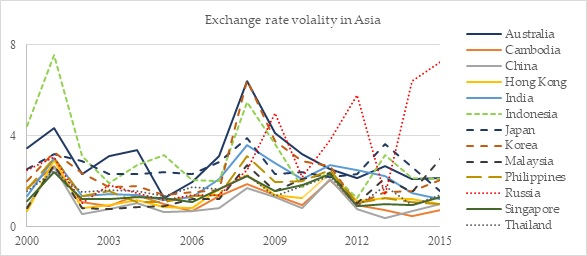
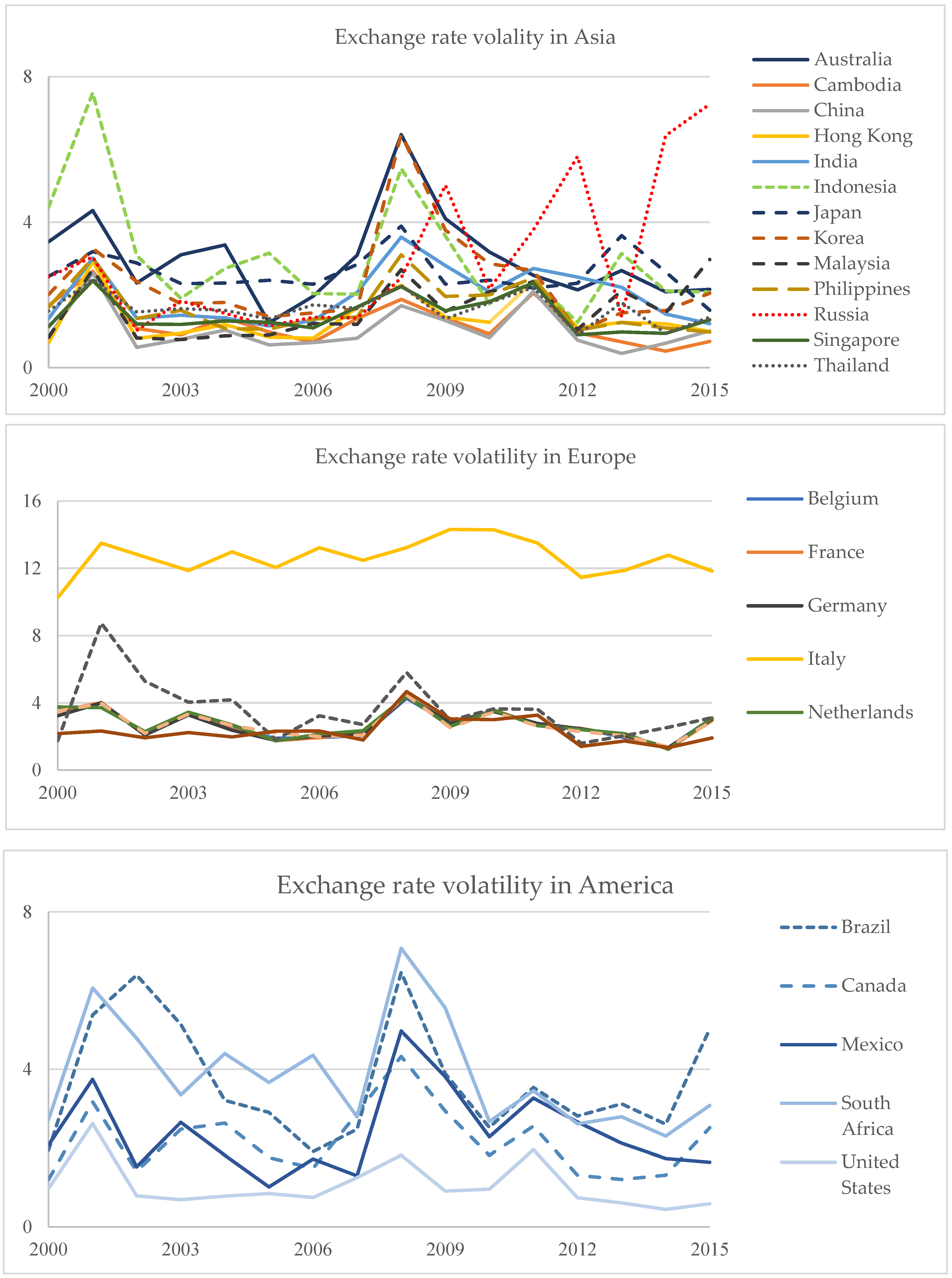
We first calculated the GARCH-based volatility for the exchange rate in terms of the monthly data and then converted it to annual data. The results and diagnostic tests for estimated the GARCH model are presented in

Table A3. Results of GARCH(1,1) model for the measure of exchange rate volatility.

Parameter	${\mathit{\alpha }}_0$		${\mathit{\alpha }}_1$		${\mathit{\beta }}_1$		${\mathit{\beta }}_2$		${\mathit{Q}}_{20}$	${\mathit{Q}}_{20}^2$	$\mathit{L}{\mathit{M}}_{20}^{\mathit{A}\mathit{R}\mathit{C}\mathit{H}}$
Australia	0.00	(0.002)	0.289 ***	(0.094)	0.235 ***	(0.082)	0.283	(0.292)	17.08	14.53	19.31
Belgium	−0.002	(0.002)	0.321 ***	(0.071)	0.024	(0.031)	0.92 ***	(0.075)	12.54	16.15	19.51
Brazil	−0.001	(0.003)	0.334 ***	(0.079)	0.329 ***	(0.114)	0.110	(0.210)	18.93	12.34	23.99
Cambodia	0.00	(0.001)	−0.127	(0.104)	0.488 ***	(0.158)	−0.009	(0.162)	22.25	13.91	10.79
Canada	−0.001	(0.002)	0.288 ***	(0.085)	0.124 ***	(0.039)	0.763 ***	(0.097)	21.66	9.72	14.69
Hong Kong	−0.002 **	(0.001)	−0.117	(0.100)	0.599 ***	(0.192)	0.332 **	(0.133)	30.51	6.03	10.34
China	0.00	(0.001)	0.045	(0.128)	0.147 **	(0.062)	0.334	(0.266)	16.14	6.85	7.48
France	−0.002	(0.002)	0.322 ***	(0.071)	0.043	(0.038)	0.903 ***	(0.077)	10.86	17.62	20.84
Germany	−0.002	(0.002)	0.319 ***	(0.071)	0.040	(0.041)	0.903 ***	(0.095)	15.03	17.17	21.47
India	0.00	(0.001)	0.082	(0.086)	0.165 *	(0.091)	0.703 ***	(0.139)	45.44	9.74	12.10
Indonesia	0.00	(0.002)	0.149 *	(0.090)	0.826 ***	(0.169)	0.136	(0.084)	19.09	17.55	9.93
Italy	0.005	(0.090)	−0.280 ***	(0.002)	−0.216 ***	(0.050)	0.359	(0.698)	9.97	24.63	22.22
Japan	−0.003 *	(0.002)	0.119	(0.081)	0.077	(0.110)	0.502	(0.749)	13.73	21.67	12.47
Korea	0.00	(0.001)	0.242 ***	(0.082)	0.218 ***	(0.075)	0.708 ***	(0.109)	12.52	9.09	11.02
Malaysia	−0.002	(0.001)	0.143	(0.088)	0.261 **	(0.104)	0.567 ***	(0.144)	17.80	5.31	6.95
Mexico	−0.003 *	(0.001)	0.173 **	(0.081)	0.343 ***	(0.070)	0.603 ***	(0.068)	28.09	11.49	8.84
Netherlands	−0.002	(0.002)	0.319 ***	(0.074)	0.013	(0.029)	0.931 ***	(0.059)	11.95	18.72	19.32
Philippines	0.00	(0.001)	0.118	(0.094)	0.134 ***	(0.048)	0.833 ***	(0.051)	17.34	14.54	11.32
Russian Federation	0.004 **	(0.002)	0.260 ***	(0.079)	0.449 ***	(0.114)	0.58 ***	(0.074)	13.31	12.40	13.79
Singapore	−0.001	(0.001)	0.065	(0.085)	0.180 ***	(0.065)	0.726 ***	(0.086)	20.80	13.36	19.78
South Africa	−0.004	(0.003)	0.267 ***	(0.095)	0.085 **	(0.040)	0.85 ***	(0.063)	21.50	16.71	17.08
Spain	−0.002	(0.002)	0.292 ***	(0.069)	0.033	(0.037)	0.916 ***	(0.078)	13.39	19.43	25.17
Thailand	−0.001	(0.001)	0.188 **	(0.074)	0.081 ***	(0.030)	−0.88 ***	(0.104)	16.92	6.96	6.57
Turkey	0.001	(0.002)	0.237 ***	(0.068)	0.601 ***	(0.145)	0.236	(0.151)	17.71	13.42	17.83
United Kingdom	−0.001	(0.002)	0.094	(0.081)	0.336 **	(0.153)	0.144	(0.265)	14.07	15.81	15.18
United States	−0.002 ***	(0.000)	−0.047	(0.099)	0.620 ***	(0.210)	0.354 **	(0.151)	35.47	6.86	10.62

The mean equation: $e_t^i={\alpha }_0+{\alpha }_1{e}_{t-1}^i+{\mu }_t^i$ and the variance equation: ${\mathrm{VOL}}_{\mathrm{GARCH}}=h_t^i={\beta }_0+{\beta }_1{\mu }_{t-1}^{i^2}+{\beta }_2{h}_{t-1}^i$. $L{M}_{20}^{ARCH}$ is the Lagrange multiplier test statistic for the null hypothesis that there is no ARCH effect up to order 20. $Q_{20}$ and $Q_{20}^2$ are the Ljung-Box statistics with lag 20 for standardized residuals and standardized residuals squared, respectively. Standard errors are numbers in the parentheses. *, **, and *** indicate the 10%, 5% and 1% significance level, respectively.

in the Appendix. Figure 3 depicts, on average, the yearly volatility of the bilateral exchange rate between Vietnam and 26 of its export partners in three different regions. The volatility fluctuates within a range of around 8%, the only exception being Italy. The magnitude of the fluctuation tends to be higher during the global crisis.

5.2. Effects of Exchange Rate Volatility on Exports

This section presents the estimation results pertaining to the effects of exchange rate volatility on manufacturing exports for the whole sample and in three regions—Asia, Europe, and America. We first show the result for the manufacturing sector, followed by its 10 subsectors.

Regarding the manufacturing sector,

Table 3. The unit root test for the full sample.

Variable	IPS	Maddala and Wu		Choi
		PP	ADF	Z	L	Pm
	Levels
GDP	0.83	0.97	0.77	0.90	0.89	0.77
Bilateral real exchange rate	0.95	0.99	0.34	0.96	0.98	0.36
VOL_GARCH	0.00	0.00	0.00	0.00	0.00	0.00
Manufacturing exports	0.06	0.42	0.00	0.00	0.00	0.00
	1st difference
GDP	0.00	0.00	0.00	0.00	0.00	0.00
Bilateral real exchange rate	0.00	0.00	0.00	0.00	0.00	0.00
VOL_GARCH	0.00	0.00	0.00	0.00	0.00	0.00
Manufacturing exports	0.00	0.00	0.00	0.00	0.00	0.00

Numbers indicate the p-values. A maximum of 2 lags were included.

and

Table 4. The unit root test for three regions.

Variable	IPS	Maddala and Wu		Choi
		PP	ADF	Z	L	Pm
Panel A: Asia	Levels
GDP	0.77	0.78	0.91	0.93	0.93	0.90
Bilateral real exchange rate	0.19	0.93	0.02	0.09	0.13	0.01
VOLGARCH	0.00	0.00	0.00	0.00	0.00	0.00
Manufacturing exports	0.12	0.47	0.00	0.04	0.02	0.00
Panel A: Asia	1st difference
GDP	0.00	0.00	0.00	0.00	0.00	0.00
Bilateral real exchange rate	0.00	0.00	0.00	0.00	0.00	0.00
VOLGARCH	0.00	0.00	0.00	0.00	0.00	0.00
Manufacturing exports	0.00	0.00	0.00	0.00	0.00	0.00
Panel B: Europe	Levels
GDP	0.46	0.89	0.32	0.38	0.33	0.35
Bilateral real exchange rate	1.00	1.00	1.00	1.00	1.00	0.98
VOLGARCH	0.00	0.00	0.73	0.50	0.51	0.75
Manufacturing exports	0.19	0.46	0.12	0.29	0.39	0.11
Panel B: Europe	1st difference
GDP	0.00	0.00	0.00	0.00	0.00	0.00
Bilateral real exchange rate	0.00	0.00	0.00	0.00	0.00	0.00
VOLGARCH	0.00	0.00	0.00	0.00	0.00	0.00
Manufacturing exports	0.00	0.00	0.00	0.00	0.00	0.00
Panel C: America	Levels
GDP	0.87	0.90	0.50	0.79	0.84	0.56
Bilateral real exchange rate	0.71	0.28	0.47	0.67	0.68	0.52
VOLGARCH	0.00	0.00	0.00	0.00	0.00	0.00
Manufacturing exports	0.29	0.31	0.00	0.00	0.00	0.00
Panel C: America	1st difference
GDP	0.05	0.06	0.08	0.06	0.06	0.06
Bilateral real exchange rate	0.00	0.02	0.00	0.00	0.00	0.00
VOLGARCH	0.00	0.00	0.00	0.00	0.00	0.00
Manufacturing exports	0.00	0.00	0.01	0.05	0.01	0.00

Numbers indicate the p-values. A maximum of 2 lags were included.

show the results of three kinds of panel unit root tests—IPS (Im et al. 2003), Maddala and Wu (1999), and Choi (2001)—for the whole sample and in three regions, respectively. At the manufacturing sector level, strong evidence of unit roots is found for the foreign GDP and real bilateral exchange rate, while, for the difference, the hypothesis that unit roots are present is strongly rejected. The variable for GARCH-based volatility is stationary for the whole sample and for Asia and America, but it contains unit roots in Europe. A similar pattern is found for manufacturing exports. Thus, the variables of interest are a mixed integration of I(0) and I(1).

The cointegration tests introduced by Pedroni (1999, 2001) were performed to determine the long-run relationship between manufacturing exports and the other variables of interest.

Table 5. The cointegration test for the full sample and three regions.

Sample	Panel v-stat	Panel rho-stat	Panel t-stat	Panel ADF-stat	Group rho-stat	Group t-stat	Group ADF-stat
Full sample	0.29	2.26 **	0.53	4.55 ***	4.35 ***	1.43	6.21 ***
Asia	0.04	1.53	0.14	3.35 ***	3.05 ***	0.87	5.11 ***
Europe	0.16	1.60	1.49	3.87 ***	2.63 ***	2.19 **	4.02 ***
America	0.42	0.64	−1.24	−0.26	1.67	−0.91	0.84

**, *** indicate the hypothesis of no cointegration is rejected at significance levels of 5%, and 1%.

displays the results for the whole sample and the three regions. Three statistics—group augmented Dickey-Fuller (ADF) test, panel ADF test, and group rho test—strongly support the hypothesis of cointegration. It is worth noting that the group small t-test and the group ADF test have a more powerful feature compared with other types of panel statistics, while the panel variance test and group rho test seem to perform poorly. Thus, based on this feature, we conclude that there is a long-run association among the given variables. An exception is the case for countries in the American region, as none of the calculated statistics are significant.

Next, we performed the long-run estimation among the relevant variables using the panel DOLS estimation in light of the confirmation by cointegration tests.

Table 6. The panel DOLS estimation for the full sample and three regions.

Variable	Full Sample	Asia	Europe	America
LnGDP	0.415 ***	0.222 *	0.831 ***	0.598
	(0.054)	(0.119)	(0.296)	(0.441)
LnREXR	−0.065 **	−0.045	−0.305	−0.163
	(0.029)	(0.066)	(0.551)	(0.354)
LnVOL	−0.829 ***	−0.312	−0.476	−1.854 **
	(0.127)	(0.463)	(0.350)	(0.805)
Constant	7.961 ***	11.236 ***	8.779 *	2.916
	(0.658)	(2.203)	(5.079)	(2.435)
Observations	413	205	125	77
R-squared	0.23	0.16	0.41	0.62

“Ln” represents variables defined in terms of logarithm. Standard errors are numbers in the parentheses. *, **, and *** indicate the 10%, 5% and 1% significance level, respectively.

presents the estimation result for the whole sample and in three regions—Asia, Europe, and America. Overall, the foreign income is found to be positively related to Vietnam’s exports for the whole sample and in Asia and Europe, as the estimated coefficients are significant at a level of at least 10%. The positive sign illustrates that an increase in income among Vietnam’ trading partners enhances the exporting performance of manufactured goods for the country. This is consistent with the trade theory that a higher income in foreign nations will lead to an increase in domestic good demands. Also, Hooy et al. (2015) asserted that Vietnam has been deeply engaged in supply chain production due to the rise of China, enhancing both economic growth and exports. According to the results of the present study, the depreciation of the Vietnam Dong is not expected to cause an adverse impact on manufacturing exports in the long run. The effect is found to be negative, although insignificant, for the three regions. Exchange rate volatility has strong reverse effects on manufacturing exports, not only for the whole sample but also in America.

We also examined the short-run relationship on the basis of the ECM model using Equation (3). The results are shown in

Table 7. The panel OLS estimation for the full sample and three regions.

Variables	Full Sample	Asia	Europe	America
ΔLnEXit−1	0.111 **	0.250 ***	0.180 *	−0.013
	(0.053)	(0.076)	(0.108)	(0.123)
ΔLnGDPit	1.351 **	1.324 *	3.607 ***	0.369
	(0.553)	(0.728)	(0.696)	(2.390)
ΔLnGDPit−1	−0.527	−0.186	−1.562 **	−2.393
	(0.516)	(0.700)	(0.769)	(1.955)
ΔLnREXRit	0.322 **	0.794 ***	−0.150	0.398
	(0.154)	(0.265)	(0.131)	(0.464)
ΔLnREXRit−1	0.210	−0.159	0.195	0.653
	(0.166)	(0.272)	(0.149)	(0.478)
ΔLnVOLit	0.024	0.045	0.042	0.072
	(0.031)	(0.041)	(0.037)	(0.095)
ΔLnVOLit−1	−0.007	0.018	0.019	−0.025
	(0.031)	(0.038)	(0.041)	(0.086)
DWTO	0.029	0.068 *	0.008	−0.044
	(0.027)	(0.038)	(0.029)	(0.081)
DCrisis	−0.186 ***	−0.301 ***	−0.118	0.118
	(0.062)	(0.081)	(0.074)	(0.201)
ECt−1	−0.234 ***	−0.257 ***	−0.185 ***	−0.716 ***
	(0.036)	(0.055)	(0.059)	(0.151)
Constant	0.166 ***	0.084 *	0.130 ***	0.369 ***
	(0.030)	(0.047)	(0.031)	(0.098)
Observations	364	182	112	70
Number of id	26	13	8	5

Δ represents variables defined in terms of difference, indicating growth rate. “Ln” represents variables defined in terms of logarithm. Standard errors are numbers in the parentheses. *, **, and *** indicate the 10%, 5% and 1% significance level, respectively.

, which paint a completely different picture of the effect of exchange rate volatility on manufacturing exports in Vietnam. The coefficients of the lagged error correction terms are negative and significant, supporting the long-run cointegration tests above. The foreign GDP and the bilateral real exchange rate have a positive association in the estimation for the whole sample and Asia. Europe has a positive significant coefficient for foreign income. The volatility of the exchange rate, on average, has no impact on exports in general in Asia, Europe, and America. The dummy variable representing the participation in the WTO is significant only for the case of Asia, implying that Vietnam gained a significant benefit in exporting goods to Asian countries. The global financial crisis is expected to be harmful, to some extent, to exports. The evidence of negative effects of volatility is weak, suggesting that it can be mostly insured against at low cost. Meanwhile, the price mechanism works via the real exchange rate to ensure that export supply equals demand. These findings imply that the manufacturing exports in Vietnam rely heavily on the partner’s income and largely benefit from the depreciation of the Vietnam Dong.

When it comes to manufacturing exports at disaggregated levels, we applied the same econometrics procedures to all 10 subsectors for the whole sample and for the three regions. Before the panel DOLS and the panel OLS estimations were run, unit root tests for stationarity and panel cointegration tests were conducted.2

The long-run effects of exchange rate volatility on each subsector for the whole sample and in the three regions are depicted in

Table 8. The panel DOLS estimation for subsectors for the whole sample.

Variable	Ln(ex1)	Ln(ex2)	Ln(ex3)	Ln(ex4)	Ln(ex5)	Ln(ex6)	Ln(ex7)	Ln(ex8)	Ln(ex9)	Ln(ex10)
LnGDP	0.449 ***	0.668 ***	0.416 ***	0.211 ***	0.570 ***	0.306 **	0.591 ***	0.824 ***	0.150 ***	0.267 *
	(0.085)	(0.125)	(0.144)	(0.047)	(0.169)	(0.127)	(0.146)	(0.141)	(0.024)	(0.149)
LnREXR	−0.099 **	0.027	−0.121	−0.213 ***	0.118	0.016	−0.163 **	−0.005	−0.139 ***	−0.184 **
	(0.046)	(0.067)	(0.077)	(0.026)	(0.092)	(0.068)	(0.079)	(0.076)	(0.013)	(0.079)
LnVOL	−0.946 ***	−0.421	−1.175 ***	−0.930 ***	−0.491	−0.879 ***	−0.776 **	−0.888 ***	−0.693 ***	−1.202 ***
	(0.203)	(0.297)	(0.341)	(0.113)	(0.403)	(0.301)	(0.349)	(0.337)	(0.057)	(0.356)
Constant	5.447 ***	5.640 ***	5.142 ***	7.102 ***	3.431	3.425 **	3.486 *	−0.222	7.255 ***	2.421
	(1.050)	(1.535)	(1.766)	(0.583)	(2.091)	(1.569)	(1.802)	(1.745)	(0.293)	(1.842)
Observations	413	413	412	412	410	408	403	411	409	403
R-squared	0.15	0.37	0.24	0.23	0.26	0.12	0.17	0.42	0.12	0.19

“Ln” represents variables defined in terms of logarithm. ex1—Food products, beverages and tobacco; ex2—Textiles, wearing apparel, leather and related products; ex3—Wood and products of wood and cork; ex4—Paper and printing; ex5—Chemicals, rubber, plastics and fuel products; ex6—Non-metallic mineral products; ex7—Basic metals and fabricated metal products; ex8—Machinery and equipment; ex9—Transport equipment; ex10—Furniture and other manufacturing. Standard errors are numbers in the parentheses. *, **, and *** indicate the 10%, 5% and 1% significance level, respectively.

and

Table 9. The panel DOLS estimation for subsectors for three regions.

Variable	Ln(ex1)	Ln(ex2)	Ln(ex3)	Ln(ex4)	Ln(ex5)	Ln(ex6)	Ln(ex7)	Ln(ex8)	Ln(ex9)	Ln(ex10)
Panel A: Asian region
LnGDP	0.284	0.477 **	0.274 *	0.101	0.294	0.107	0.355 *	0.901 ***	−0.081	−0.063
	(0.189)	(0.186)	(0.145)	(0.117)	(0.286)	(0.176)	(0.214)	(0.193)	(0.179)	(0.152)
LnREXR	0.074	−0.102	−0.005	−0.141 **	0.071	0.062	−0.102	0.066	−0.109	0.040
	(0.106)	(0.104)	(0.081)	(0.066)	(0.161)	(0.097)	(0.120)	(0.109)	(0.101)	(0.085)
LnVOL	0.015	−0.347	−0.389	−0.853 *	0.316	0.019	0.055	−0.968	0.300	0.173
	(0.739)	(0.726)	(0.566)	(0.461)	(1.133)	(0.688)	(0.849)	(0.761)	(0.704)	(0.597)
Panel B: European region
LnGDP	1.351 ***	0.700 **	0.738 *	0.811 **	1.014 **	0.639	1.363 ***	0.880 ***	0.581 **	1.239 ***
	(0.448)	(0.279)	(0.442)	(0.344)	(0.404)	(0.509)	(0.335)	(0.278)	(0.227)	(0.297)
LnREXR	−2.317 ***	0.262	−0.393	−1.516 **	0.585	0.489	0.008	0.191	−0.820 *	−0.211
	(0.834)	(0.520)	(0.823)	(0.641)	(0.753)	(0.947)	(0.628)	(0.518)	(0.425)	(0.547)
LnVOL	−0.690	−0.438	−0.285	−0.305	−0.487	−0.543	−0.218	−0.409	−0.287	−0.082
	(0.529)	(0.329)	(0.522)	(0.406)	(0.477)	(0.600)	(0.396)	(0.328)	(0.270)	(0.343)
Panel C: American region
LnGDP	1.119 **	0.807 ***	0.354	1.210 ***	0.198	0.361	0.387	0.440	0.225	1.181
	(0.531)	(0.309)	(0.655)	(0.363)	(0.713)	(0.585)	(0.511)	(0.389)	(0.750)	(0.941)
LnREXR	−0.615	−0.175	0.071	−0.402	0.315	0.898 *	0.182	0.461	0.267	−0.195
	(0.426)	(0.248)	(0.519)	(0.291)	(0.572)	(0.470)	(0.405)	(0.312)	(0.602)	(0.686)
LnVOL	−1.039	−1.833 ***	−2.166 *	−0.075	−2.482 *	−0.873	−2.319 **	−1.420 **	−1.617	−1.064
	(0.970)	(0.564)	(1.214)	(0.662)	(1.301)	(1.073)	(0.951)	(0.713)	(1.374)	(1.862)

“Ln” represents variables defined in terms of logarithm. ex1—Food products, beverages and tobacco; ex2—Textiles, wearing apparel, leather and related products; ex3—Wood and products of wood and cork; ex4—Paper and printing; ex5—Chemicals, rubber, plastics and fuel products; ex6—Non-metallic mineral products; ex7—Basic metals and fabricated metal products; ex8—Machinery and equipment; ex9—Transport equipment; ex10—Furniture and other manufacturing. Standard errors are numbers in the parentheses. *, **, and *** indicate the 10%, 5% and 1% significance level, respectively.

, respectively. Based on all of the data in Table 8, 8 out of 10 manufacturing subsectors suffered adverse effects due to exchange rate volatility. The coefficients of two subsectors, namely, textiles, wearing apparel, leather, and related products and chemicals, rubber, plastics, and fuel products, are statistically insignificant although negative. The effect of the bilateral real exchange rate is also found to be negative in five subsectors in the long run. Thus, a depreciation policy in Vietnam would lead to a decline in export value in the long term as it generates volatility in the exchange rate.

When the geographical factor is taken into consideration, we observe a completely different picture of the relationship between exchange rate devaluation, exchange rate volatility, and export performance at the subsector level. As can be seen from Table 9, exchange rate volatility has almost no effect on exports in Asia and Europe, but America has five subsectors that are negatively related to the exchange rate volatility.3 It is only the subsector of non-metallic mineral products in the American region that enjoys a favorable gain from exchange rate depreciation without being influenced by the exchange rate fluctuation.

Using Equation (3), the short-run effects of exchange rate volatility on export performance at disaggregated levels were regressed and are provided in the next four tables with the application of panel estimation.

Table 10. The panel OLS estimation for subsectors for the full sample.

Variable	ΔLnEX1	ΔLnEX2	ΔLnEX3	ΔLnEX4	ΔLnEX5	ΔLnEX6	ΔLnEX7	ΔLnEX8	ΔLnEX9	ΔLnEX10
ΔLnEXit−1	0.169 ***	0.124 ***	0.042	0.056	0.030	0.087 *	0.068	0.024	−0.040	0.047
	(0.050)	(0.044)	(0.050)	(0.049)	(0.043)	(0.049)	(0.048)	(0.051)	(0.043)	(0.050)
ΔLnGDPit	2.967 ***	2.118 ***	−0.389	2.223 ***	2.098 **	4.597 ***	3.854 **	4.289 ***	2.859 **	5.465 ***
	(1.142)	(0.467)	(1.185)	(0.844)	(0.871)	(1.070)	(1.853)	(0.878)	(1.417)	(1.797)
ΔLnGDPit−1	−3.374 ***	−0.682	0.510	−0.436	−0.348	−0.175	−0.721	−0.902	−0.609	−1.603
	(1.041)	(0.435)	(1.073)	(0.773)	(0.790)	(0.984)	(1.732)	(0.808)	(1.302)	(1.628)
ΔLnREXRit	0.062	0.049	0.159	−0.262	0.291	0.269	0.845	0.023	−0.166	−0.912 *
	(0.318)	(0.130)	(0.331)	(0.238)	(0.245)	(0.300)	(0.516)	(0.247)	(0.388)	(0.500)
ΔLnREXRit−1	0.175	0.297 **	−0.129	0.219	−0.014	−0.325	−0.270	0.189	0.401	1.619 ***
	(0.333)	(0.136)	(0.344)	(0.246)	(0.261)	(0.313)	(0.543)	(0.255)	(0.419)	(0.527)
ΔLnVOLit	0.030	−0.033	−0.037	0.062	0.088 *	−0.078	0.098	−0.053	0.273 ***	−0.080
	(0.065)	(0.027)	(0.068)	(0.048)	(0.050)	(0.062)	(0.106)	(0.050)	(0.079)	(0.102)
ΔLnVOLit−1	−0.041	0.018	−0.089	0.028	−0.091 *	−0.063	0.108	0.040	0.092	0.041
	(0.063)	(0.026)	(0.066)	(0.047)	(0.051)	(0.060)	(0.107)	(0.049)	(0.080)	(0.100)
DWTO	0.093 *	−0.015	−0.122 **	−0.050	−0.052	−0.039	0.064	0.035	−0.036	0.077
	(0.056)	(0.023)	(0.058)	(0.041)	(0.043)	(0.052)	(0.090)	(0.043)	(0.068)	(0.089)
DCrisis	−0.005	−0.061	−0.014	−0.189 **	−0.047	0.045	−0.607 ***	−0.134	−0.840 ***	0.101
	(0.126)	(0.052)	(0.132)	(0.095)	(0.097)	(0.119)	(0.203)	(0.097)	(0.155)	(0.200)
ECt−1	−0.255 ***	−0.262 ***	−0.431 ***	−0.357 ***	−0.309 ***	−0.345 ***	−0.452 ***	−0.385 ***	−0.378 ***	−0.422 ***
	(0.036)	(0.030)	(0.045)	(0.041)	(0.040)	(0.038)	(0.047)	(0.046)	(0.048)	(0.050)
Constant	0.239 ***	0.139 ***	0.243 ***	0.190 ***	0.159 ***	0.073	0.197 **	0.034	0.313 ***	−0.032
	(0.061)	(0.025)	(0.063)	(0.046)	(0.048)	(0.057)	(0.100)	(0.047)	(0.077)	(0.097)
Observations	364	364	363	363	361	359	353	362	360	349

Δ represents variables defined in terms of difference, indicating growth rate. ex1—Food products, beverages and tobacco; ex2—Textiles, wearing apparel, leather and related products; ex3—Wood and products of wood and cork; ex4—Paper and printing; ex5—Chemicals, rubber, plastics and fuel products; ex6—Non-metallic mineral products; ex7—Basic metals and fabricated metal products; ex8—Machinery and equipment; ex9—Transport equipment; ex10—Furniture and other manufacturing. Standard errors are numbers in the parentheses. *, **, and *** indicate the 10%, 5% and 1% significance level, respectively.

presents the result for the whole sample. The bilateral real exchange rate has a favorable impact on exports in such subsectors as (i) textiles, wearing apparel, leather, and related products and (ii) furniture and other manufacturing products. This implies that depreciation boosts exports in the short run rather than in the long run in some subsectors. Similarly, exchange rate volatility is found to be positively associated with exports for the subsector of transport equipment. Exporters in this subsector may pursue a strategy of exporting more in order to maintain its trading value, as hypothesized by De Grauwe (1988). The subsector of chemicals, rubber, plastics, and fuel products is found to be quite sensitive to exchange rate volatility in the short run, given that its estimated coefficient is positive in the current period but becomes negative in the first lag. We find no statistically significant effect of exchange rate depreciation and volatility on export values for the eight remaining subsectors.

A significantly different pattern is seen in Asia, Europe, and America, as indicated in

Table 11. The panel OLS estimation for subsectors for the Asian region.

Variable	ΔLnEX1	ΔLnEX2	ΔLnEX3	ΔLnEX4	ΔLnEX5	ΔLnEX6	ΔLnEX7	ΔLnEX8	ΔLnEX9	ΔLnEX10
ΔLnEXit−1	0.227 ***	0.052	0.333 ***	0.005	−0.031	0.135 **	0.125 *	−0.005	−0.122 *	0.213 ***
	(0.069)	(0.063)	(0.069)	(0.068)	(0.064)	(0.069)	(0.070)	(0.073)	(0.067)	(0.063)
ΔLnGDPit	2.943 **	1.375 **	0.543	2.411 **	1.480	2.747	4.327 *	5.482 ***	3.961 **	3.711 **
	(1.408)	(0.662)	(1.144)	(1.001)	(0.928)	(1.691)	(2.563)	(1.401)	(1.827)	(1.791)
ΔLnGDPit−1	−2.216 *	0.648	−0.280	−0.385	−0.121	0.735	−2.043	−1.957	−1.578	−2.116
	(1.320)	(0.605)	(1.074)	(0.926)	(0.863)	(1.562)	(2.421)	(1.317)	(1.702)	(1.655)
ΔLnREXRit	0.364	0.264	1.265 ***	0.634 *	1.014 ***	0.992	−0.232	0.427	0.229	0.205
	(0.510)	(0.234)	(0.414)	(0.372)	(0.343)	(0.624)	(0.942)	(0.520)	(0.676)	(0.645)
ΔLnREXRit−1	−0.489	−0.137	−0.004	0.160	−0.219	0.045	1.020	0.640	1.222 *	0.815
	(0.510)	(0.233)	(0.422)	(0.364)	(0.354)	(0.609)	(0.935)	(0.510)	(0.691)	(0.643)
ΔLnVOLit	0.053	−0.003	−0.048	0.108 *	0.107 **	−0.074	0.050	−0.037	0.318 ***	−0.172 *
	(0.081)	(0.037)	(0.065)	(0.057)	(0.053)	(0.098)	(0.145)	(0.080)	(0.103)	(0.103)
ΔLnVOLit−1	−0.010	−0.030	0.054	0.101 *	0.035	−0.019	0.136	0.066	0.097	0.040
	(0.074)	(0.034)	(0.061)	(0.053)	(0.050)	(0.089)	(0.136)	(0.074)	(0.098)	(0.095)
DWTO	0.133 *	0.030	0.040	−0.018	−0.003	−0.026	0.063	0.138 *	−0.037	0.019
	(0.073)	(0.033)	(0.059)	(0.051)	(0.048)	(0.087)	(0.132)	(0.072)	(0.093)	(0.094)
DCrisis	−0.027	−0.077	−0.089	−0.162	−0.283 ***	0.226	−0.471 *	−0.158	−0.967 ***	−0.338 *
	(0.153)	(0.070)	(0.125)	(0.111)	(0.101)	(0.183)	(0.276)	(0.152)	(0.203)	(0.196)
ECt−1	−0.251 ***	−0.162 ***	−0.708 ***	−0.266 ***	−0.370 ***	−0.388 ***	−0.468 ***	−0.424 ***	−0.277 ***	−0.435 ***
	(0.048)	(0.044)	(0.075)	(0.052)	(0.068)	(0.053)	(0.072)	(0.069)	(0.064)	(0.066)
Constant	0.099	0.084 **	0.067	0.133 **	0.183 ***	0.107	0.195	−0.023	0.333 ***	0.075
	(0.091)	(0.042)	(0.073)	(0.065)	(0.061)	(0.109)	(0.167)	(0.090)	(0.119)	(0.119)
Observations	182	182	182	181	179	178	177	181	180	179

Δ represents variables defined in terms of difference, indicating growth rate. ex1—Food products, beverages and tobacco; ex2—Textiles, wearing apparel, leather and related products; ex3—Wood and products of wood and cork; ex4—Paper and printing; ex5—Chemicals, rubber, plastics and fuel products; ex6—Non-metallic mineral products; ex7—Basic metals and fabricated metal products; ex8—Machinery and equipment; ex9—Transport equipment; ex10—Furniture and other manufacturing. Standard errors are numbers in the parentheses. *, **, and *** indicate the 10%, 5% and 1% significance level, respectively.

,

Table 12. The panel OLS estimation for subsectors for the European region.

Variable	ΔLnEX1	ΔLnEX2	ΔLnEX3	ΔLnEX4	ΔLnEX5	ΔLnEX6	ΔLnEX7	ΔLnEX8	ΔLnEX9	ΔLnEX10
ΔLnEXit−1	0.223 **	0.426 ***	−0.134 *	0.116	−0.152 *	0.194 **	−0.123	0.223 **	−0.016	0.029
	(0.099)	(0.095)	(0.081)	(0.094)	(0.082)	(0.097)	(0.093)	(0.107)	(0.056)	(0.109)
ΔLnGDPit	7.087 ***	2.848 ***	6.238 ***	5.563 ***	5.233 ***	6.088 ***	2.002	4.141 ***	0.445	4.602
	(2.364)	(0.737)	(1.825)	(1.797)	(1.125)	(1.193)	(4.198)	(1.207)	(2.561)	(4.079)
ΔLnGDPit−1	−6.557 ***	−2.943 ***	0.289	1.943	−0.239	0.027	−0.269	−1.274	−0.214	0.700
	(1.910)	(0.675)	(1.420)	(1.408)	(0.838)	(1.099)	(3.299)	(0.919)	(2.021)	(3.104)
ΔLnREXRit	−0.604	−0.117	−1.276 ***	0.087	−0.268	−0.154	2.072 ***	−0.218	−0.675	−0.725
	(0.446)	(0.142)	(0.345)	(0.336)	(0.223)	(0.227)	(0.784)	(0.225)	(0.465)	(0.771)
ΔLnREXRit−1	0.232	0.380 **	−0.161	−0.522	−0.521 **	−0.402	−0.026	−0.146	0.732	0.801
	(0.512)	(0.165)	(0.398)	(0.388)	(0.242)	(0.261)	(0.953)	(0.253)	(0.549)	(0.896)
ΔLnVOLit	0.015	0.035	0.052	−0.165 *	0.085	−0.179 ***	0.275	−0.045	0.275 **	−0.034
	(0.128)	(0.039)	(0.097)	(0.096)	(0.060)	(0.066)	(0.216)	(0.064)	(0.130)	(0.225)
ΔLnVOLit−1	−0.017	0.134 ***	−0.340 ***	−0.171	−0.099	−0.178 **	−0.016	−0.121	0.390 **	−0.012
	(0.143)	(0.045)	(0.111)	(0.109)	(0.089)	(0.074)	(0.294)	(0.074)	(0.175)	(0.248)
DWTO	0.098	−0.032	−0.214 ***	−0.085	−0.074	0.028	0.075	0.002	−0.011	0.243
	(0.102)	(0.030)	(0.074)	(0.072)	(0.047)	(0.049)	(0.166)	(0.048)	(0.102)	(0.173)
DCrisis	0.057	−0.088	0.588 ***	0.011	0.026	−0.050	−0.456	0.057	−1.215 ***	0.424
	(0.259)	(0.080)	(0.194)	(0.192)	(0.125)	(0.129)	(0.443)	(0.128)	(0.260)	(0.437)
ECt−1	−0.430 ***	−0.261 ***	−0.632 ***	−0.645 ***	−0.290 ***	−0.227 ***	−0.448 ***	−0.401 ***	−0.409 ***	−0.411 ***
	(0.091)	(0.061)	(0.104)	(0.111)	(0.086)	(0.063)	(0.104)	(0.089)	(0.096)	(0.111)
Constant	0.182 *	0.124 ***	0.153 *	0.110	0.070	−0.058	0.244	−0.008	0.348 ***	−0.235
	(0.104)	(0.033)	(0.081)	(0.082)	(0.056)	(0.054)	(0.191)	(0.054)	(0.119)	(0.186)
Observations	112	112	112	112	112	112	108	112	111	111

Δ represents variables defined in terms of difference, indicating growth rate. ex1—Food products, beverages and tobacco; ex2—Textiles, wearing apparel, leather and related products; ex3—Wood and products of wood and cork; ex4—Paper and printing; ex5—Chemicals, rubber, plastics and fuel products; ex6—Non-metallic mineral products; ex7—Basic metals and fabricated metal products; ex8—Machinery and equipment; ex9—Transport equipment; ex10—Furniture and other manufacturing. Standard errors are numbers in the parentheses. *, **, and *** indicate the 10%, 5% and 1% significance level, respectively.

and

Table 13. The panel OLS estimation for subsectors for the American region.

Variable	ΔLnEX1	ΔLnEX2	ΔLnEX3	ΔLnEX4	ΔLnEX5	ΔLnEX6	ΔLnEX7	ΔLnEX8	ΔLnEX9	ΔLnEX10
ΔLnEXit−1	0.130	0.134	0.088	0.102	0.134	−0.076	0.174	0.020	0.006	−0.152
	(0.124)	(0.100)	(0.134)	(0.119)	(0.104)	(0.116)	(0.118)	(0.120)	(0.132)	(0.118)
ΔLnGDPit	−0.737	2.376	−4.055	4.259	0.168	10.412 **	6.723	−0.085	9.043	26.903 ***
	(4.799)	(1.818)	(7.342)	(3.717)	(5.163)	(4.251)	(6.912)	(3.239)	(6.431)	(10.124)
ΔLnGDPit−1	−3.140	−2.437	5.179	−5.242 *	−1.020	−7.540 **	0.025	3.905	1.298	−3.896
	(3.990)	(1.540)	(5.591)	(3.022)	(4.120)	(3.458)	(5.721)	(2.558)	(5.168)	(8.156)
ΔLnREXRit	−0.357	−0.053	2.859 **	−0.880	1.308	0.900	0.139	0.209	1.222	−5.376 ***
	(0.960)	(0.351)	(1.336)	(0.692)	(0.947)	(0.782)	(1.289)	(0.600)	(1.197)	(1.792)
ΔLnREXRit−1	0.302	0.666 **	−1.484	1.383 **	0.794	−0.830	−0.498	0.593	−0.526	4.882 ***
	(0.877)	(0.325)	(1.169)	(0.618)	(0.902)	(0.738)	(1.158)	(0.539)	(1.098)	(1.620)
ΔLnVOLit	0.006	−0.117	0.323	0.339 **	0.285	0.242	−0.157	−0.169	0.637 **	−0.007
	(0.189)	(0.074)	(0.262)	(0.145)	(0.198)	(0.164)	(0.268)	(0.126)	(0.253)	(0.353)
ΔLnVOLit−1	−0.178	0.137 *	0.013	0.099	−0.294	0.089	0.355	0.120	0.223	0.098
	(0.173)	(0.075)	(0.246)	(0.131)	(0.194)	(0.151)	(0.259)	(0.117)	(0.231)	(0.338)
DWTO	−0.086	−0.126 **	−0.170	0.067	−0.070	−0.123	−0.087	−0.049	0.016	0.231
	(0.165)	(0.064)	(0.226)	(0.122)	(0.170)	(0.141)	(0.229)	(0.112)	(0.212)	(0.331)
DCrisis	0.118	−0.126	−0.000	−0.119	0.661	0.054	−1.191 **	−0.293	0.390	1.513 *
	(0.396)	(0.152)	(0.550)	(0.311)	(0.413)	(0.339)	(0.548)	(0.256)	(0.522)	(0.799)
ECt−1	−0.618 ***	−0.520 ***	−0.516 ***	−0.514 ***	−0.393 ***	−0.315 **	−0.596 ***	−0.411 ***	−0.656 ***	−0.605 ***
	(0.141)	(0.089)	(0.115)	(0.126)	(0.112)	(0.130)	(0.127)	(0.116)	(0.164)	(0.163)
Constant	0.531 ***	0.312 ***	0.389	0.235	0.265	0.258	0.301	0.113	0.089	−0.546
	(0.198)	(0.076)	(0.266)	(0.151)	(0.210)	(0.179)	(0.287)	(0.140)	(0.270)	(0.399)
Observations	70	70	69	70	70	69	68	69	69	59

Δ represents variables defined in terms of difference, indicating growth rate. ex1—Food products, beverages and tobacco; ex2—Textiles, wearing apparel, leather and related products; ex3—Wood and products of wood and cork; ex4—Paper and printing; ex5—Chemicals, rubber, plastics and fuel products; ex6—Non-metallic mineral products; ex7—Basic metals and fabricated metal products; ex8—Machinery and equipment; ex9—Transport equipment; ex10—Furniture and other manufacturing. Standard errors are numbers in the parentheses. *, **, and *** indicate the 10%, 5% and 1% significance level, respectively.

, respectively. The short-run effects of exchange rate volatility vary considerably across the subsectors, as well as in the given regions. Asia has three subsectors that are positively associated with exchange rate volatility, together with one that reacts negatively. In Europe, the number of subsectors experiencing favorable and harmful effects is three and two, respectively. In America, 3 out of 10 subsectors are found to be positively related to exchange rate fluctuations. Interesting to note is that the export performance in the subsector of Transport equipment is observed to benefit from the exchange rate fluctuations, as its estimated coefficients are statistically positive in all three regions. There is an increase in the export performance of textiles, wearing apparel, leather, and related products to countries in Europe and America when the exchange rate is volatile. The Paper and printing subsector is negatively related to the exchange rate fluctuations in Asia but positively associated in Europe. Other subsectors, such as (i) wood and products of wood and cork, (ii) Chemicals, rubber, plastics, and fuel products, (iii) Non-metallic mineral products, and (iv) Furniture and other manufacturing products are influenced by exchange rate volatility, either positively or negatively.

In the short run, the impact of the bilateral exchange rate on the export performance at disaggregated levels is considerably different across the regions. When the real bilateral exchange devaluates, it raises Vietnam’s export value in three subsectors—textiles, wearing apparel, leather, and related products; wood and products of wood and cork; and paper and printing—to countries in Europe and America, and it has no effect on the remaining subsectors. In Europe, the estimated results indicate that two subsectors are positively influenced by exchange rate fluctuations, another two react negatively, and results for the rest of the subsectors are inconclusive. All results prove that the impact of the exchange rate on exports at the manufacturing disaggregated level depends on two factors: (i) the type of export and (ii) the exporting destination.

6. Concluding Remarks

Intensive debates have taken place on the impact of currency depreciation on Vietnam’s export performance in recent years. Many may support this strategy because it is argued that doing so will enhance export performance, whereas others assert that the policy could lead to exchange rate volatility, which, in turn, is harmful to exports. This study was conducted to shed light on the link between exchange rate volatility and exports between Vietnam and 26 of its key export partners for the 2001–2015 period using data from the disaggregated level for both the manufacturing sector and its 10 subsectors.

Key findings from this empirical study are as follows. First, with regard to the manufacturing sector, the strategy of devaluing the VND provides a positive impact on Vietnam’s manufacturing exports in the short run, but it creates exchange rate volatility, causing a decline in export value in the long run. In the short run, this strategy is beneficial only for the exports to Asian countries, while there is no supporting evidence for a clear short-run effect for all three regions—Asia, Europe, and America. Exchange rate volatility is, on average, harmful in the long run, especially when the exporting destination is a European country. Interestingly, no influence on export performance is shown in the short run for either the whole sample or the three subsamples. Second, Vietnam’s manufacturing exports benefit from an increase in foreign income, as well as its participation in the WTO, to some extent. Meanwhile, the global financial crisis hindered the export value of the manufacturing sectors in Vietnam, as expected. Third, with regard to 10 specific subsectors in Vietnam, exchange rate volatility has negative effects on export performance for most of them in the long run, whereas mixed evidence is found for some in the short run.

On balance, the findings from this study confirm that, in the context of Vietnam, the level of the bilateral real exchange rate between the VND and other currencies is far more important than currency volatility for enhancing export performance for Vietnam in the short run. Thus, Vietnam’s authorities could take advantage of depreciation to enhance exports, thus balancing the current net trade. Yet, intervention involving the exchange rate market should be conducted with caution, as it causes fluctuations in exchange rates, resulting in poor export performance in the long run. Also, it should be noted that at disaggregated levels, exchange rate volatility seems to cause more harm to exporters to the American region than to Asian and European partners, especially in some specific subsectors. Thus, it is suggested that exporters to American markets in these sectors use hedging instruments in the derivatives market to maintain their targeted export value and profitability.

There are some shortcomings in the current study. First, it is possible that exchange rate devaluation, volatility, and export performance have a reversed causal relationship with one another. When there are problems with exports, the exchange rate reacts more severely with greater depreciation, thus making exchange rates more volatile. Second, the effect of increases and decreases in exchange rate volatility on exports may be considerably different, raising the asymmetric effect. Nishimura and Hirayama (2013) find an asymmetric effect of the level of exchange rate and the volatility have different effects on bilateral exports between China and Japan. Thus, it would be worth taking those issues into consideration in future research using higher-frequency data, especially for a small open dynamic country like Vietnam. The country has targeted its exports as an important factor in boosting economic growth and is becoming increasingly integrated into the region and the world.

References

- Aftab, Muhammad, Karim Bux Shah Syed, Rubi Ahmad, and Izlin Ismail. 2015. Exchange-rate variability and industry trade flows between Malaysia and Japan. The Journal of International Trade & Economic Development 25: 453–78. [Google Scholar]
- Aftab, Muhammad, Karim Bux Shah Syed, and Naveed Akhter Katper. 2017. Exchange-rate volatility and Malaysian-Thai bilateral industry trade flows. Journal of Economic Studies 44: 99–114. [Google Scholar] [CrossRef]
- Aristotelous, Kyriacos. 2001. Exchange-rate volatility, exchange-rate regime, and trade volume: Evidence from the UK–US export function (1889–1999). Economics Letters 72: 87–94. [Google Scholar] [CrossRef]
- Asteriou, Dimitrios, Kaan Masatci, and Keith Pılbeam. 2016. Exchange rate volatility and international trade: International evidence from the MINT countries. Economic Modelling 58: 133–40. [Google Scholar] [CrossRef]
- Atif, Rao Muhammad, Liu Haiyun, and Haider Mahmood. 2017. Pakistan’s agricultural exports, determinants and its potential: An application of stochastic frontier gravity model. The Journal of International Trade & Economic Development 26: 257–76. [Google Scholar]
- Bahmani-Oskooee, Mohsen, and Yongqing Wang. 2007. United States-China trade at the commodity level and the Yuan-Dollar exchange rate. Contemporary Economic Policy 25: 341–61. [Google Scholar] [CrossRef]
- Bahmani-Oskooee, Mohsen, Marzieh Bolhassani, and Scott Hegerty. 2012. Exchange-rate volatility and industry trade between Canada and Mexico. The Journal of International Trade & Economic Development 21: 389–408. [Google Scholar]
- Bahmani-Oskooee, Mohsen, Hanafiah Harvey, and Scott W. Hegerty. 2013. The effects of exchange-rate volatility on commodity trade between the US and Brazil. The North American Journal of Economics and Finance 25: 70–93. [Google Scholar] [CrossRef]
- Chit, Myint Moe. 2008. Exchange rate volatility and exports: Evidence from the ASEAN-China Free Trade Area. Journal of Chinese Economic and Business Studies 6: 261–77. [Google Scholar] [CrossRef]
- Chit, Myint Moe, Marian Rizov, and Dirk Willenbockel. 2010. Exchange rate volatility and exports: New empirical evidence from the emerging East Asian economies. The World Economy 33: 239–63. [Google Scholar] [CrossRef]
- Choi, In. 2001. Unit Root Tests for Panel Data. Journal of International Money and Finance 20: 249–72. [Google Scholar] [CrossRef]
- Choudhry, Taufiq, and Syed S. Hassan. 2015. Exchange rate volatility and UK imports from developing countries: The effect of the global financial crisis. Journal of International Financial Markets, Institutions and Money 39: 89–101. [Google Scholar] [CrossRef] [Green Version]
- Clark, Peter B. 1973. Uncertainty, exchange risk, and the level of international trade. Western Economic Journal 6: 302–13. [Google Scholar] [CrossRef]
- De Grauwe, Paul. 1988. Exchange rate variability and the slowdown in growth of international trade. IMF Staff Papers 35: 63–84. [Google Scholar] [CrossRef]
- De Vita, Glauco, and Andrew Abbott. 2004. The impact of exchange rate volatility on UK exports to EU countries. Scottish Journal of Political Economy 51: 62–81. [Google Scholar] [CrossRef]
- Erdem, Ekrem, Saban Nazlioglu, and Cumhur Erdem. 2010. Exchange rate uncertainty and agricultural trade: Panel cointegration analysis for Turkey. Agricultural Economics 41: 537–43. [Google Scholar] [CrossRef]
- Hansen, Peter R., and Asger Lunde. 2005. A forecast comparison of volatility models: Does anything beat a GARCH(1,1)? Journal of Applied Econometrics 20: 873–89. [Google Scholar] [CrossRef]
- Hayakawa, Kazunobu, and Fukunari Kimura. 2009. The effect of exchange rate volatility on international trade in East Asia. Journal of the Japanese and International Economies 23: 395–406. [Google Scholar] [CrossRef]
- Hooper, Peter, and Steven W. Kohlhagen. 1978. The effect of exchange rate uncertainty on the prices and volume of international trade. Journal of International Economics 8: 483–511. [Google Scholar] [CrossRef]
- Hooy, Chee-Wooi, Law Siong-Hook, and Chan Tze-Haw. 2015. The impact of the Renminbi real exchange rate on ASEAN disaggregated exports to China. Economic Modelling 47: 253–59. [Google Scholar] [CrossRef]
- Hsu, Kuang-Chung, and Hui-Chu Chiang. 2011. The threshold effects of exchange rate volatility on exports: Evidence from US bilateral exports. The Journal of International Trade & Economic Development 20: 113–28. [Google Scholar]
- Ilzetzki, Ethan, Carmen M. Reinhart, and Kenneth S. Rogoff. 2017. Exchange arrangements entering the 21st century: Which anchor will hold? National Bureau of Economic Research. [Google Scholar] [CrossRef]
- Im, Kyung So, M. Hashem Pesaran, and Yongcheol Shin. 2003. Testing for unit roots in heterogeneous panels. Journal of Econometrics 115: 53–74. [Google Scholar] [CrossRef]
- Kandilov, Ivan T. 2008. The effects of exchange rate volatility on agricultural trade. American Journal of Agricultural Economics 90: 1028–43. [Google Scholar] [CrossRef]
- Maddala, Gangadharrao S., and Shaowen Wu. 1999. A comparative study of unit root tests with panel data and a new simple test. Oxford Bulletin of Economics and Statistics 61: 631–52. [Google Scholar] [CrossRef]
- Narayan, Seema, and Tri Tung Nguyen. 2016. Does the trade gravity model depend on trading partners? Some evidence from Vietnam and her 54 trading partners. International Review of Economics & Finance 41: 220–37. [Google Scholar]
- Nguyen, Dong Xuan. 2016. Trade liberalization and export sophistication in Vietnam. The Journal of International Trade & Economic Development 25: 1071–89. [Google Scholar]
- Nishimura, Yusaku, and Kenjiro Hirayama. 2013. Does exchange rate volatility deter Japan-China trade? Evidence from Pre-and Post-exchange rate reform in China. Japan and the World Economy 25: 90–101. [Google Scholar] [CrossRef]
- Pedroni, Peter. 1999. Critical values for cointegration tests in heterogeneous panels with multiple regressors. Oxford Bulletin of Economics and Statistics 61: 653–70. [Google Scholar] [CrossRef]
- Pedroni, Peter. 2001. Purchasing power parity tests in cointegrated panels. The Review of Economics and Statistics 83: 727–31. [Google Scholar] [CrossRef]
- Prasad, Eswar, Kenneth Rogoff, Shang-Jin Wei, and M. Ayhan Kose. 2003. Effects of financial globalization on developing countries: Some empirical evidence. IMF Occasional Paper 220: 201–28. [Google Scholar]
- Sercu, Piet. 1992. Exchange risk, exposure, and the option to trade. Journal of International Money and Finance 11: 579–93. [Google Scholar]
- Sercu, Piet, and Cynthia Vanhulle. 1992. Exchange rate volatility, international trade, and the value of exporting firms. Journal of Banking and Finance 16: 155–82. [Google Scholar] [CrossRef]
- Soleymani, Abdorreza, and Soo Y. Chua. 2014. Effect of exchange rate volatility on industry trade flows between Malaysia and China. The Journal of International Trade & Economic Development 23: 626–55. [Google Scholar]
- Viaene, Jean-Marie, and Casper De Vries. 1992. International trade and exchange rate volatility. European Economic Review 36: 1311–21. [Google Scholar] [CrossRef]
- Vieira, Flavio Vilela, and Ronald MacDonald. 2016. Exchange rate volatility and exports: A panel data analysis. Journal of Economic Studies 43: 203–21. [Google Scholar] [CrossRef]
- Xiong, Bo. 2017. The Impact of TPP and RCEP on tea exports from Vietnam: The case of Tariff elimination and pesticide policy cooperation. Agricultural Economics 8: 413–24. [Google Scholar] [CrossRef]
- Xuan, Nguyen Thanh, and Yuqing Xing. 2008. Foreign Direct Investment and exports: The experiences of Vietnam. Economics of Transition 16: 183–97. [Google Scholar] [CrossRef]