The Role of Diversity on Linear Scattering Operator: The Case of Strip Scatterers Observed under the Fresnel Approximation

Abstract

The aim of this paper is to investigate the role of multiple views and multiple frequencies in linear inverse scattering problems. The study was performed assuming the Fresnel-zone approximation on the scattering operator. Due to the crucial role played by singular values into analysing the linear inverse scattering problems, the impact of view and frequency diversities on singular values behaviour was established. In fact, the singular values were related to the most common metrics used to quantify the achievable performances in inverse scattering problems, such as the number of degrees of freedom (NDF), the information content and the resolution.

1. Introduction

In this paper, linear [1] inverse scattering problems are addressed. Their aim is to reconstruct an unknown target from measures of its scattered field when the scattering scene is illuminated by a known incident field. As is well known, such problem is ill-posed in sense of the Hadamard [2]. This means that, even when the uniqueness of solution is guaranteed, the noise affecting the data can be amplified on the unknown space resulting in meaningless solutions. Accordingly, to mitigate the effect of noise, regularisation techniques are mandatory [3], which allow obtaining approximate solutions resulting from a trade-off between accuracy and stability. Hence, although these methods control noise propagation to obtain stable solutions, they preclude the possibility of retrieving arbitrary details about the unknown.

It is known that probing the scattering scene at different incidence directions (multi-view configuration) and/or at different frequencies (multi-frequency configuration) improves the achievable performance [4]. However, some degree of redundancy is expected due to the reciprocity and when the problem is overdetermined. That is, data collected by employing one or two diversities (view and/or frequency) are not necessarily all independent.

In this paper, the role played by the view and frequency diversities on the achievable performance is analysed. To address such a purpose, the singular values decomposition of the scattering operator [5] is a very powerful mathematical tool. This is because: firstly, all regularisation schemes result in a proper filtering of the scattering operator singular spectrum [3]; and, secondly, the most common figures of merits, namely the resolution [6], the Number of Degree of Freedom (NDF) [7] and the information content [8,9], that allow assessing the performance in linear inverse problem can be expressed in terms of it.

In fact, the point-spread function whose main lobe is related to the resolution can be expressed in terms of the singular functions of the scattering operator spanning the unknown space [10].

The number of degrees of freedom (NDF) that represents the number of independent data required to represent the field with a given degree of accuracy can be evaluated as the number of singular values greater than a threshold depending on the noise [11]. More in detail, such a parameter allows us to gain insightful information about many aspects of the problem. For instance, it is strictly linked to the achievable resolution as the dimension of the set of the field that can be represented with the assigned accuracy and also it identifies the subspace of scatterers that can be correctly reconstructed. It can give a measure on how complicated the design of an optical system can be [12]. By interpreting the scattering operator as a propagator of information, the NDF has also been linked to the number of independent channels of communication which significantly connect (i.e., with coupling coefficient higher than a noise dependent threshold) the scattering and the measurement volumes [13,14,15,16,17]. By following further the information point of view, for many times the NDF has been considered a measure of the information that can be conveyed back from scattered field measurements to the scatterer [18,19]. However, although the NDF is linked to the information content, they actually are not the same thing [20].

A measure of information content can be given by exploiting two main approaches: the Shannon information theory [8] or the Kolmogorov information theory [9]. The choice between these is based on prior information about the unknown space, the data space and their mapping. However, regardless of the approach exploited, the information content can be expressed in terms of the number of significant singular values (NDF) and their numerical value [21,22,23].

According to the above discussion, our purpose becomes to assess the impact of the diversities on the singular values decomposition of the scattering operator. In [4], the same analysis is carried out when the far-field approximation is assumed. Such an approximation puts serious restrictions on the size of the investigation domain and/or the distance from the latter and observation domain. Therefore, here, the aim is to expand previous studies in order to cover configurations which are under the Fresnel approximation. In particular, our aim is to know the singular values of the relevant scattering operator in closed form and to link their behaviour to the scattering parameters. Unfortunately, as in [4], we cannot fill such a gap. Instead, by exploiting the same mathematical tools shown in [4], we succeed in introducing upper and lower bounds for the singular values and linking their behaviour to configuration parameters.

The paper is organised as follows: In Section 2, some mathematical notations and concepts are introduced. In Section 3, the analysis about view and frequency diversities is developed. Finally, a conclusive summary ends the paper.

2. Notation and Mathematical Preliminaries

The aim of this section is to provide some mathematical preliminaries and notations that are used in the following sections. The set of all the complex valued functions $f\left(x\right)$ supported on $I\in \mathbb{R}$ that are square integrable is denoted as ${\mathcal{L}}_I^2$. According to the Plancherel Theorem, the Fourier transform of such functions can be introduced

$$F\left(u\right)={\int }_{I}f\left(x\right)e^{-jux}dx$$

(1)

where u is the space frequency. Let the operator ${\mathcal{B}}_{\mathsf{\Omega }}$ be the band limiting projector such that

$${\mathcal{B}}_{\mathsf{\Omega }}f\left(x\right)=\frac{1}{2\pi }{\int }_{\mathsf{\Omega }}F\left(u\right)e^{jux}du$$

(2)

where $\mathsf{\Omega }$ is a single compact interval not necessarily centred around the zero frequency. Similarly, the space limiting projector ${\mathcal{P}}_I$ is given by

$${\mathcal{P}}_{I}f\left(x\right)=\left\{\begin{array}{cc}f\left(x\right),\hfill & x\in I\hfill \\ 0,\hfill & x\notin I.\hfill \end{array}\right.$$

(3)

Let us consider the operator ${\mathcal{P}}_I{\mathcal{B}}_{\mathsf{\Omega }}{\mathcal{P}}_{I}f\left(x\right)$. If $\mathsf{\Omega }$ and I are both centred around zero, its explicit form is given by

$${\mathcal{P}}_I{\mathcal{B}}_{\mathsf{\Omega }}{\mathcal{P}}_{I}f\left(x\right)={\int }_{-m\left(I\right)/2}^{m\left(I\right)/2}\frac{sin\left[m\right(\mathsf{\Omega })/2(x-y)]}{\pi (x-y)}f\left(y\right)dy$$

(4)

where $m\left(I\right)$ and $m\left(\mathsf{\Omega }\right)$ are the measures of the intervals I and $\mathsf{\Omega }$, respectively. As well known [24,25], the operator in Equation (4) is a compact self-adjoint positive definite operator and its eigenspectrum is given in terms of prolate spheroidal wave-functions $u_n={\varphi }_n(c,x)/\sqrt{{\eta }_n\left(c\right)}$, where $c=m\left(I\right)m\left(\mathsf{\Omega }\right)/4$ is the so-called spatial-bandwidth product, ${\varphi }_n(c,x)$ is the nth prolate function and ${\eta }_n\left(c\right)$ are the corresponding eigenvalues. The latter exhibit a step-like behaviour: they are almost constant to one until the index reaches $N=[2c/\pi ]$, with $[·]$ being the greater integer lower than its argument. Beyond this index, they decay exponentially to zero. The eigenvalues hold the same when $\mathsf{\Omega }$ and/or I are not centred intervals, whereas the eigenfunctions are linked to the previous ones by unitary transformations (phase changes and/or translations).

For our purposes, it is useful to consider also the sum operator

$$\mathcal{S}={\alpha }_1{\mathcal{P}}_I{\mathcal{B}}_{{\mathsf{\Omega }}_1}{\mathcal{P}}_I+{\alpha }_2{\mathcal{P}}_I{\mathcal{B}}_{{\mathsf{\Omega }}_2}{\mathcal{P}}_I$$

(5)

where ${\mathsf{\Omega }}_1$ and ${\mathsf{\Omega }}_2$ are disjoint bands and ${\alpha }_1$ and ${\alpha }_2$ are amplitude factors. The eigensystem of Equation (5) is not known in closed form. However, in [26], it is shown that it can be very well approximated by the union of the eigensystems of each single operator appearing in Equation (5). Indeed, if $c_1$ and $c_2$ are both greater than 4, then

$${\mathcal{P}}_I{\mathcal{B}}_{{\mathsf{\Omega }}_1}{\mathcal{P}}_I{u}_{n2}\cong 0$$

$${\mathcal{P}}_I{\mathcal{B}}_{{\mathsf{\Omega }}_2}{\mathcal{P}}_I{u}_{n1}\cong 0$$

(6)

where $u_{n1}$ and $u_{n2}$ are the eigenfuctions of ${\mathcal{P}}_I{\mathcal{B}}_{{\mathsf{\Omega }}_1}{\mathcal{P}}_I$ and ${\mathcal{P}}_I{\mathcal{B}}_{{\mathsf{\Omega }}_2}{\mathcal{P}}_I$, respectively (note that the equality can never occur because the operators are positive definite and hence have empty null spaces). Accordingly, the eigensystem of Equation (5) can be approximated as

$$\left\{\begin{array}{c}\left\{u_n\left[\mathcal{S}\right]\right\}=\left\{u_{n1}\right\}\cup \left\{u_{n2}\right\}\hfill \\ \left\{{\lambda }_n\left[\mathcal{S}\right]\right\}=\left\{{\alpha }_1{\eta }_n\left(c_1\right)\right\}\cup \left\{{\alpha }_2{\eta }_n\left(c_2\right)\right\}\hfill \end{array}\right.$$

(7)

Thus, the ${\lambda }_n\left[\mathcal{S}\right]$ exhibit a two-step like behaviour. The first knee occurs at $[2c_1/\pi ]$ (when ${\alpha }_1>{\alpha }_2$) or $[2c_2/\pi ]$ (for ${\alpha }_2>{\alpha }_1$), whereas the second one is at $[2c_1/\pi ]+[2c_2/\pi ]$. Moreover, the first eigenvalue jump is related to the ration ${\alpha }_1/{\alpha }_2$.

A useful theorem to estimate upper and lower bounds for the eigenvalues of a convolution operator is introduced:

Theorem 1.

Let $\mathcal{A}$ and $\mathcal{B}$ be two compact operators belonging to the space of linear operators $H(\mathcal{X},\mathcal{Y})$, $\mathcal{X}=L_X^2$ and $\mathcal{Y}=L_Y^2$ being Hilbert spaces of square integrable functions supported over X and Y. If

$$\langle {\mathcal{A}}^{†}\mathcal{A}f,f\rangle \le \langle {\mathcal{B}}^{†}\mathcal{B}f,f\rangle \forall f\in \mathcal{X}$$

then say ${\lambda }_n[{\mathcal{A}}^{†}\mathcal{A}]$ and ${\lambda }_n[{\mathcal{B}}^{†}\mathcal{B}]$ the eigenvalues of ${\mathcal{A}}^{†}\mathcal{A}$ and ${\mathcal{B}}^{†}\mathcal{B}$

$${\lambda }_n[{\mathcal{A}}^{†}\mathcal{A}]\le {\lambda }_n[{\mathcal{B}}^{†}\mathcal{B}]\forall n$$

Its proof is reported in Appendix of the paper [27].

Consider a convolution operator

$$\mathcal{G}:f\left(x\right)\in L_I^2⟶g\left(y\right)={\int }_{I}k(y-x)f\left(x\right)dx\in L_I^2$$

(8)

with the band-limited kernel function $k\left(x\right)\in L_{\mathbb{R}}^2$. This is a Hilbert–Schmidt operator and, thus, it is compact. Let $K\left(u\right)$ be the Fourier transform of $k\left(y\right)$. $K\left(u\right)$ is assumed to be a real and positive function with compact support $\mathsf{\Omega }=[u_{min},u_{max}]$. Divide now the bandwidth $\mathsf{\Omega }$ in M sub-bands ${\mathsf{\Omega }}_m$ each of width $\Delta =(u_{max}-u_{min})/M$ such that ${\mathsf{\Omega }}_m\bigcap {\mathsf{\Omega }}_n=0$ for $m\ne n$ and $\mathsf{\Omega }={\bigcup }_m{\mathsf{\Omega }}_m$. Further, let us consider the two sequences

$${\tilde{K}}_1,{\tilde{K}}_2,\dots {\tilde{K}}_m,\dots {\tilde{K}}_M,$$

(9)

and

$${\widehat{K}}_1,{\widehat{K}}_2,\dots {\widehat{K}}_m,\dots {\widehat{K}}_M,$$

(10)

where

$${\tilde{K}}_m=\underset{{\mathsf{\Omega }}_m}{max}\left\{K\left(u\right)\right\},$$

and

$${\widehat{K}}_m=\underset{{\mathsf{\Omega }}_m}{min}\left\{K\left(u\right)\right\}.$$

After introducing two “auxiliary” operators written as

$$\tilde{\mathcal{G}}f\left(x\right)=\sum _{m=1}^m{\tilde{K}}_m{\mathcal{P}}_I{\mathcal{B}}_{{\mathsf{\Omega }}_m}{\mathcal{P}}_{I}f\left(x\right)$$

(11)

$$\widehat{\mathcal{G}}f\left(x\right)=\sum _{m=1}^M{\widehat{K}}_m{\mathcal{P}}_I{\mathcal{B}}_{{\mathsf{\Omega }}_m}{\mathcal{P}}_{I}f\left(x\right)$$

(12)

the following proposition, consequence of Theorem 1, can be stated [28]:

say ${\lambda }_n[\tilde{\mathcal{G}}]$, ${\lambda }_n[\widehat{\mathcal{G}}]$ and ${\lambda }_n[\mathcal{G}]$ the eigenvalues of $\tilde{\mathcal{G}}$, $\widehat{\mathcal{G}}$ and $\mathcal{G}$, respectively. Then, it can be shown that

$${\lambda }_n[\widehat{\mathcal{G}}]\le {\lambda }_n\left(\mathcal{G}\right)\le {\lambda }_n[\tilde{\mathcal{G}}]\hspace{1em}\forall n.$$

(13)

3. Mathematical Formulation

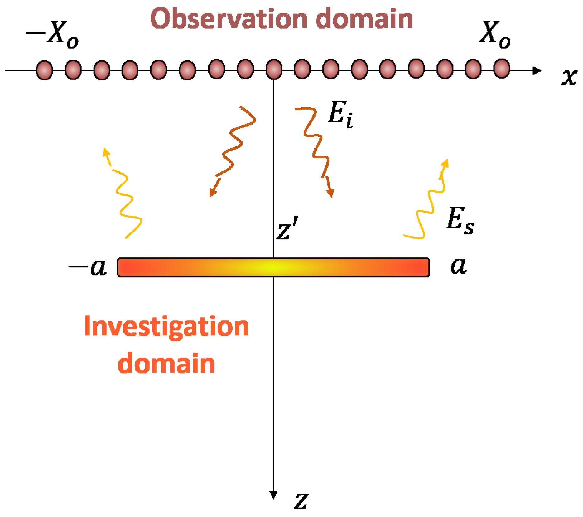
Consider the two dimensional scattering configuration shown in Figure 1. A strip scatterer is supported over the interval $I=[-a,a]$ along the x-axis, located at $z=z^{\prime }$. Invariance is assumed along the polarisation direction of the incident field, which in turn is orthogonal to the strip. The scattering scene is illuminated by a filamentary current located at $x_i$ on the x-axis. Moreover, along the interval $O=[-X_o,X_o]$ of the same axis, the only y component of the scattered field is collected in Fresnel zone.

When a multi-view measurement configuration is exploited, one can take advantage of incident field coming from different directions to improve the performance achievable in the reconstruction. Suppose obtaining such a multi-view configuration by moving the current position $x_i$ along the interval $S_i\subseteq O$.

Instead, when the frequency diversity is exploited, the illumination frequency varies within the interval $[f_{min},f_{max}]$ that corresponds to the interval $S_k=[k_{min},k_{max}]$ of the wavenumber domain. Accordingly, under the Fresnel approximation, the scattering operator is (apart from some unessential scalar factors)

$${\mathcal{A}}_{if}:\chi \left(x\right)\in {\mathcal{L}}_I^2⟶E_S(x_o,x_i,k)=\frac{1}{z^{\prime }}{\int }_{-a}^a{e}^{-j(2k{z}^{\prime }+\frac{k}{2z^{\prime }}{(x_o-x^{\prime })}^2+\frac{k}{2z^{\prime }}{(x_i-x^{\prime })}^2)}\chi (x^{\prime })d{x}^{\prime }\in {\mathcal{L}}_{(O\times S_i\times S_k)}^2$$

(14)

When only view or frequency diversity is exploited, the corresponding operators are denoted as ${\mathcal{A}}_i$ and ${\mathcal{A}}_f$, respectively. To obtain the singular values of the scattering operator, the following eigenvalues problem must be solved

$${\mathcal{A}}_l^{†}{\mathcal{A}}_l{u}_{ln}={\lambda }_n{u}_{ln}$$

(15)

with $l=\{i,f\}$, ${\mathcal{A}}_l^{†}$ being the adjoint operator of ${\mathcal{A}}_l$. In fact, it is well known that the singular values ${\sigma }_n[{\mathcal{A}}_l]$ of ${\mathcal{A}}_l$ are equal to $\sqrt{{\lambda }_n[{\mathcal{A}}_l^{†}{\mathcal{A}}_l]}$, while $u_{ln}$ are the right singular functions of ${\mathcal{A}}_l$.

3.1. View Diversity

In this section, the impact of view diversity on the singular values of the scattering operator is analysed. Accordingly, suppose that the scattered field is collected for different directions of the incident field and at a single frequency. The scattering operator is

$${\mathcal{A}}_i:\chi \left(x\right)\in {\mathcal{L}}_I^2\to E_s(x_o,x_i)=\frac{1}{z^{\prime }}{\int }_{-a}^a{e}^{-j(2k_0{z}^{\prime }+\frac{k_0}{2z^{\prime }}{(x_o-x^{\prime })}^2+\frac{k_0}{2z^{\prime }}{(x_i-x^{\prime })}^2)}\chi (x^{\prime })d{x}^{\prime }\in {\mathcal{L}}_{(O\times S_i)}^2$$

(16)

where $k_0$ is the wavenumber at the fixed frequency.

At first, let us suppose that $S_i$ is a discrete subset of O. Let M be the number of views taken by uniformly sampling O. Thus, the left side of Equation (15) is written as

$${\mathcal{A}}_i^{†}{\mathcal{A}}_i{u}_{in}=\sum _{m=1}^M\frac{\lambda }{z^{\prime }}{\mathcal{T}}^{†}{\mathcal{P}}_I{\mathcal{B}}_{{\mathsf{\Omega }}_m}{\mathcal{P}}_I\mathcal{T}{u}_{in}$$

(17)

where $\mathcal{T}$ is an unitary operator defined as

$${\mathcal{T}}_{k_0}:u_{in}\in L_I^2⟶{\overline{u}}_{in}(x,k_0)=e^{-j\frac{k_0}{z^{\prime }}{x}^2}{u}_{in}(x)\in L_I^2$$

(18)

${\mathsf{\Omega }}_m=\left[\frac{k_0}{z^{\prime }}{x}_{im}-\frac{k_0}{z^{\prime }}{X}_o,\frac{k_0}{z^{\prime }}{x}_{im}+\frac{k_0}{z^{\prime }}{X}_o\right]$. The unitary operator ${\mathcal{T}}_{k_0}$ does not affect the eigenvalues of ${\mathcal{A}}_i^{†}{\mathcal{A}}_i$ but introduces a phase term on $u_{in}\left(x\right)$. Accordingly, by including such a phase term in the eigenfunctions, the eigenvalues problem in Equation (15) is equivalent to

$${\mathcal{A}}_i^{†}{\mathcal{A}}_i{\overline{u}}_{in}={\lambda }_n{\overline{u}}_{in}$$

(19)

where, now,

$${\mathcal{A}}_i^{†}{\mathcal{A}}_i{\overline{u}}_{in}=\sum _{m=1}^M\frac{\lambda }{z^{\prime }}{\mathcal{P}}_I{\mathcal{B}}_{{\mathsf{\Omega }}_m}{\mathcal{P}}_I{\overline{u}}_{in}$$

(20)

For simplicity, consider the case of $M=2$ and $M=3$. In the first case, $S=\{-X_o,X_o\}$ and (20) becomes

$${\mathcal{A}}_i^{†}{\mathcal{A}}_i{\overline{u}}_{in}=\frac{\lambda }{z^{\prime }}{\mathcal{P}}_I{\mathcal{B}}_{{\mathsf{\Omega }}_1}{\mathcal{P}}_I{\overline{u}}_{in}+\frac{\lambda }{z^{\prime }}{\mathcal{P}}_I{\mathcal{B}}_{{\mathsf{\Omega }}_2}{\mathcal{P}}_I{\overline{u}}_{in}.$$

(21)

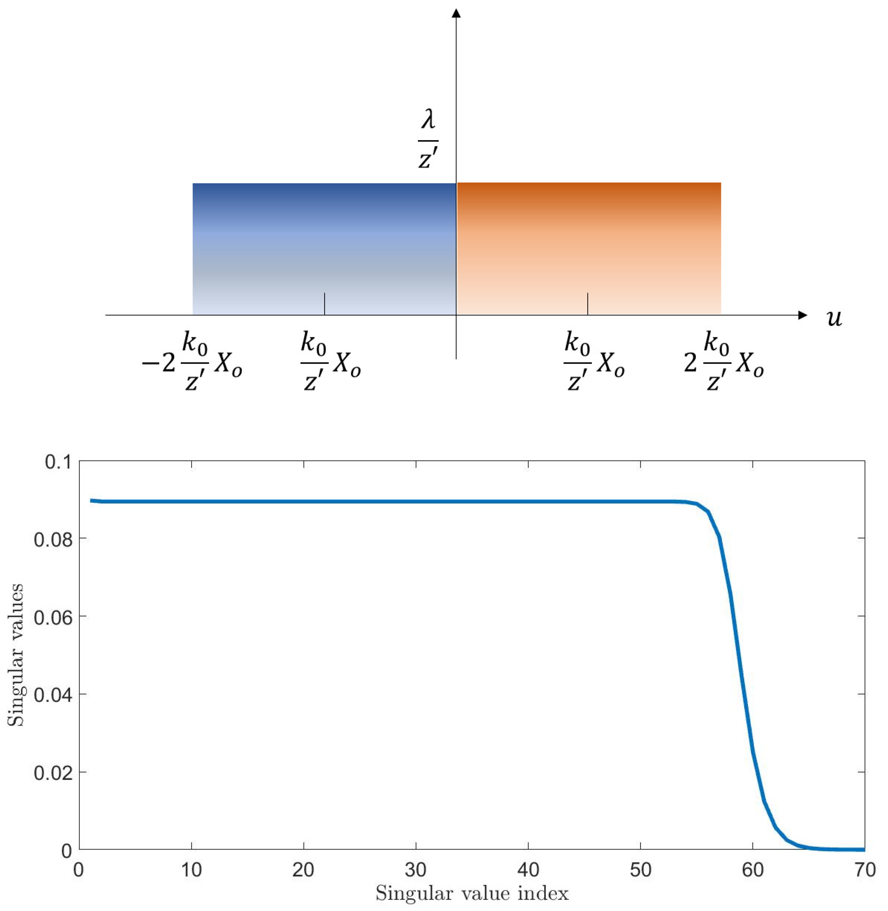
Now, since the two considered views are the extremal once (at $-X_o$ and $X_o$), ${\mathsf{\Omega }}_1\cap {\mathsf{\Omega }}_2=\varnothing$ and Equation (7) holds. Accordingly, the eigenvalues ${\lambda }_n[{\mathcal{A}}_i^{\ast }{\mathcal{A}}_i]$ exhibit a step-like behaviour with a flat part equal to $\frac{\lambda }{z^{\prime }}$ until the index $N=2\left[\frac{2c}{\pi }\right]$ with $c=a\frac{k_0}{z^{\prime }}{X}_o$, and after they decay exponentially. The same behaviour can be also observed for the singular values of the scattering operator. This single step behaviour allows identifying N as the number of degrees of freedom (NDF) ideally independent on the noise. By comparing such result with respect to the single view configuration, it is evident that adopting two different views, equal to the extremal ones, entails doubling the NDF. An example of this result is shown in Figure 2.

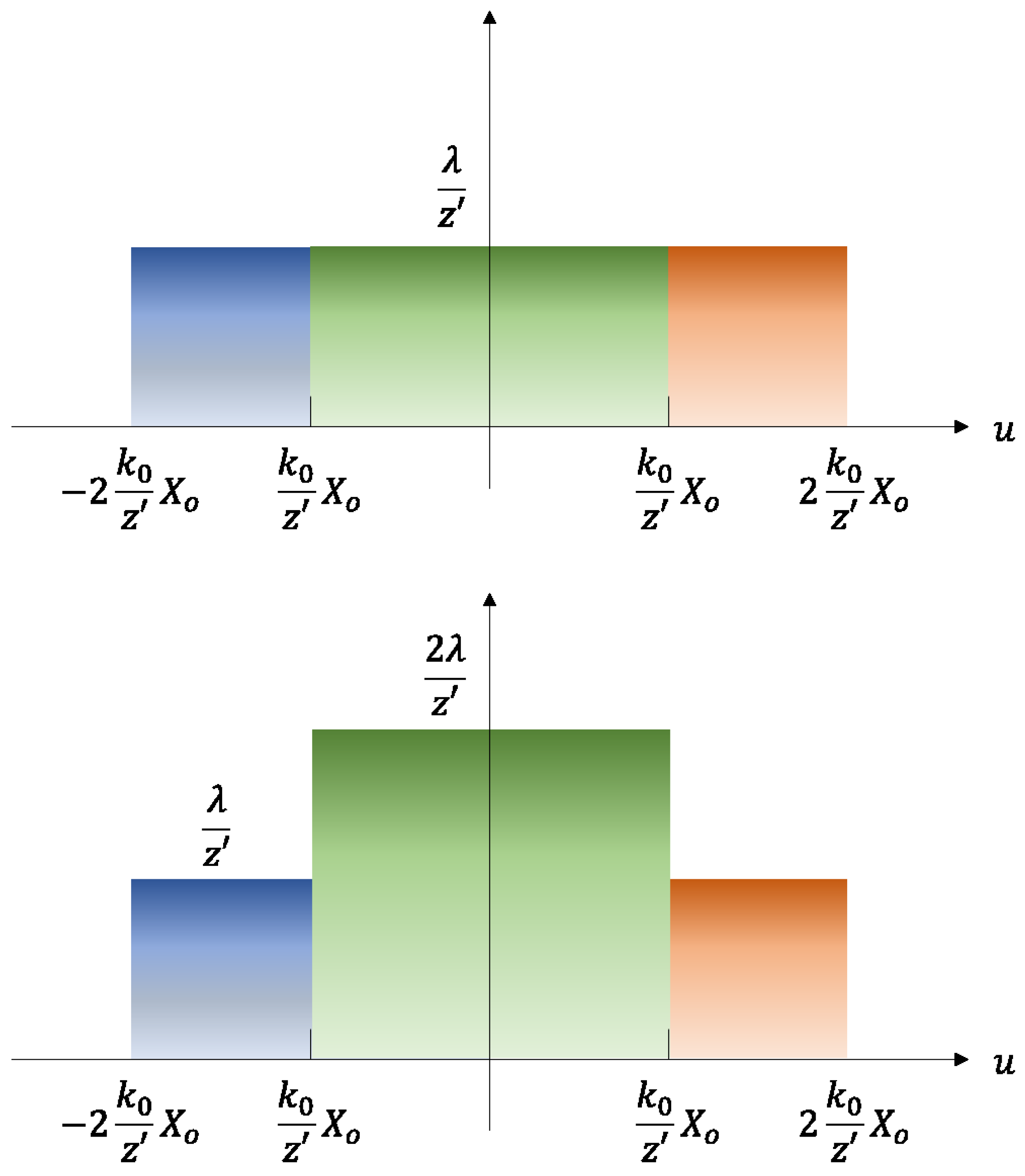
Consider the case of $M=3$, since the discrete set of views is $S_i=\{-X_o,0,X_o\}$, Equation (20) becomes

$${\mathcal{A}}_i^{†}{\mathcal{A}}_i{\overline{u}}_{in}=\sum _{m=1}^3\frac{\lambda }{z^{\prime }}{\mathcal{P}}_I{\mathcal{B}}_{{\mathsf{\Omega }}_m}{\mathcal{P}}_I{\overline{u}}_{in}$$

(22)

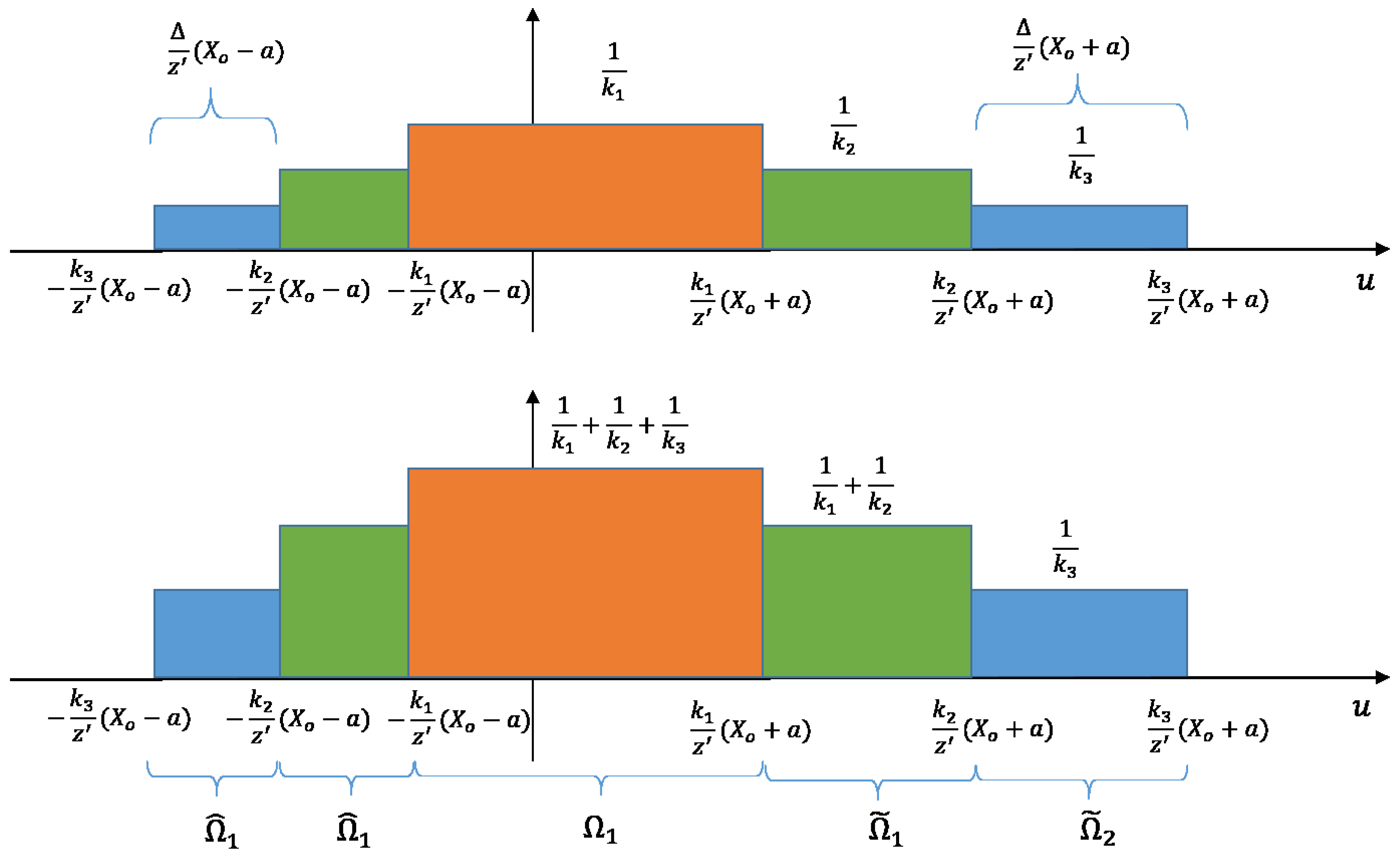
where ${\mathsf{\Omega }}_1=\left[-2\frac{k_0}{z^{\prime }}{X}_o,0\right]$, ${\mathsf{\Omega }}_2=\left[-\frac{k_0}{z^{\prime }}{X}_o,\frac{k_0}{z^{\prime }}{X}_o\right]$ and ${\mathsf{\Omega }}_3=\left[0,2\frac{k_0}{z^{\prime }}{X}_o\right]$. This situation is slightly different from the one addressed above. This is because for $M=3$ the bands ${\mathsf{\Omega }}_m$ overlap and the result given in Equation (7) cannot be exploited. However, such an inconvenience can be overcome by recasting those bands to make them disjoint. In fact, instead of ${\mathsf{\Omega }}_1$, ${\mathsf{\Omega }}_2$ and ${\mathsf{\Omega }}_3$, the operator ${\mathcal{A}}_i^{\ast }{\mathcal{A}}_i$ can be expressed in terms of the disjoint bands ${\tilde{\mathsf{\Omega }}}_1=\left[-\frac{k_0}{z^{\prime }}{X}_o,\frac{k_0}{z^{\prime }}{X}_o\right]$, ${\tilde{\mathsf{\Omega }}}_2=\left[-2\frac{k_0}{z^{\prime }}{X}_o,-\frac{k_0}{z^{\prime }}{X}_o\right]$ and ${\tilde{\mathsf{\Omega }}}_3=\left[\frac{k_0}{z^{\prime }}{X}_o,2\frac{k_0}{z^{\prime }}{X}_o\right]$. Figure 3 gives some explanations about the recasting of the bands. In particular, the top panel shows the Fourier transform of the kernel functions of each operator appearing in Equation (22), and the bottom one their overlapping. Accordingly, Equation (22) can be rewritten as

$${\mathcal{A}}_i^{\ast }{\mathcal{A}}_i{\overline{u}}_{in}=\frac{\lambda }{z^{\prime }}{\mathcal{P}}_I{\mathcal{B}}_{{\tilde{\mathsf{\Omega }}}_1}{\mathcal{P}}_I{\overline{u}}_{in}+2\frac{\lambda }{z^{\prime }}{\mathcal{P}}_I{\mathcal{B}}_{{\tilde{\mathsf{\Omega }}}_2}{\mathcal{P}}_I{\overline{u}}_{in}+\frac{\lambda }{z^{\prime }}{\mathcal{P}}_I{\mathcal{B}}_{{\tilde{\mathsf{\Omega }}}_3}{\mathcal{P}}_I{\overline{u}}_{in}.$$

(23)

Now, Equation (7) holds. Hence, as long as $c_1=c_3=a\frac{k_0}{2z^{\prime }}{X}_o>4$ and $c_2=a\frac{k_0}{z^{\prime }}{X}_o>4$, the eigenvalues of the operator in Equation (23) (and, thus, also the singular values) exhibit a two-step behaviour with knees occurring at the indexes $N_1=\left[\frac{2c_1}{\pi }\right]$ and $N_2=\left[N_1+\frac{2c_2}{\pi }+\frac{2c_3}{\pi }\right]$. Unlike before, a non-uniform increase in the singular values level can be observed that shapes the singular values behaviour so as to make the NDF dependent on the truncation threshold (hence, noise dependent). This affects the information metrics positively. In fact, having fixed the noise, higher singular values can lead to a more stable inversion procedure. However, the number of singular values different from zero does not change with respect to the the case of two extremal views.

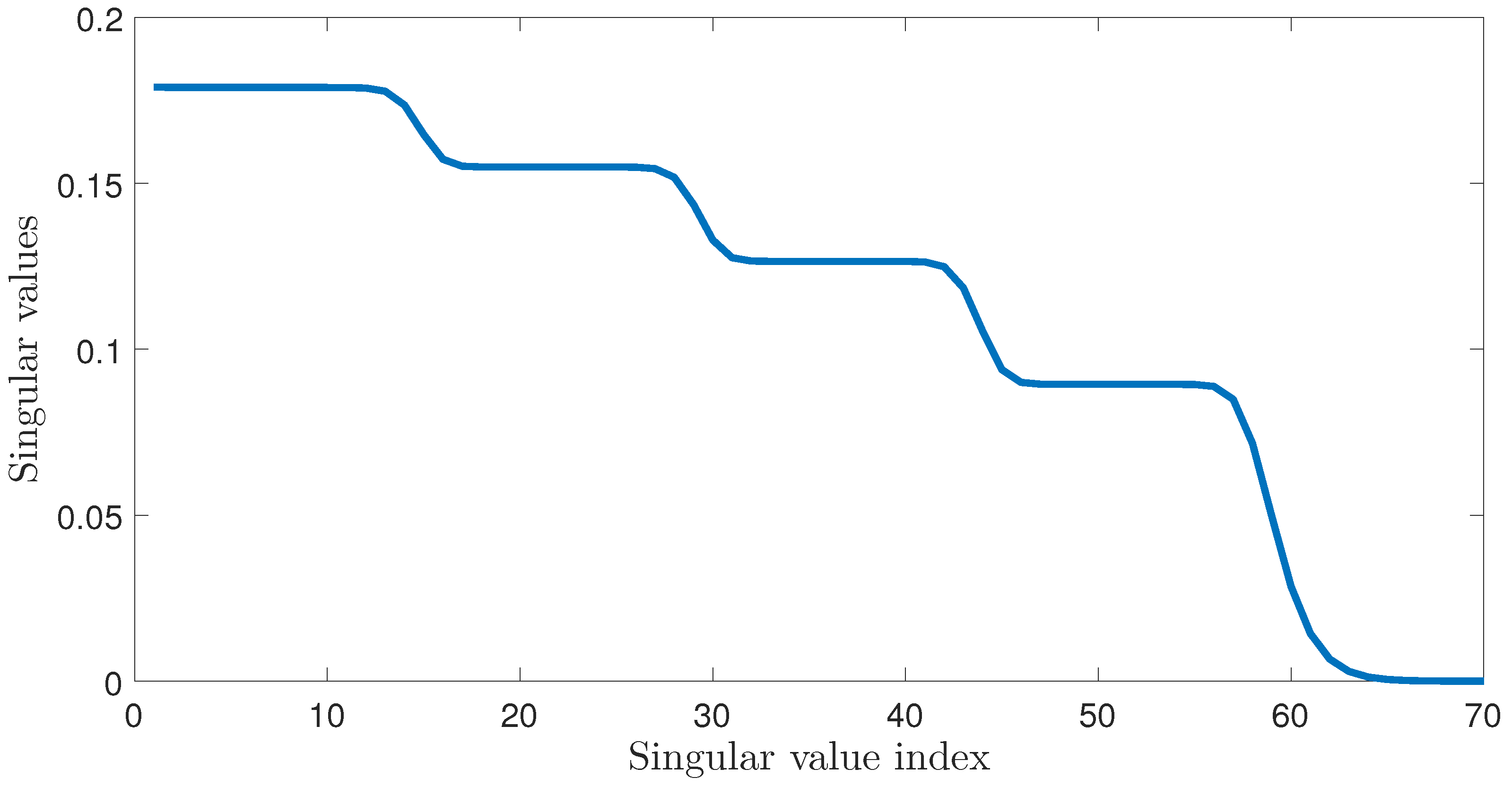
The same reasoning can also be applied to a generic number M (for simplicity odd) of views taken uniformly in O. The Fourier transform of the kernel of operator in Equation (20) is a band-limited function with support on $[-2\frac{k_0}{z^{\prime }}{X}_o,2\frac{k_0}{z^{\prime }}{X}_o]$ and consists in $2M-3$ steps. In particular, each step is supported over a spatial frequency interval $\Delta =\frac{2\frac{k_0}{z^{\prime }}{X}_o}{M-1}$ in size except for the one centred around the frequency zero, which is $2\Delta$ large. Accordingly, the singular values exhibit a $(M-1)$ step-like behaviour and the number of singular values on each step is $4\frac{c_M}{\pi }$ with $c_M=a\Delta /2$. Moreover, on the mth step the singular values are equal to $\sqrt{(M-m)\frac{\lambda }{z^{\prime }}}$ with $m=\{1,\dots ,M-1\}$. This result is very well verified by the example reported in Figure 4.

The singular values exhibit the expected $M-1=4$ steps and their value estimation is also in strict accordance to the numerical result. For example, on the first step, the previous formula returns $0.178$, which well agrees with the value given by the numerical simulation. Hence, summarising, the results obtained show that the maximum number of significant (different from zero) singular values can be obtained by using only two views at $-X_o$ and $X_o$, while introducing more views increases the singular values level. The latter affects positively the performances because it makes the reconstruction more stable against the noise.

Let us consider the case of views varying continuously, so that $S_i=O$ and the operator ${\mathcal{A}}_i^{†}{\mathcal{A}}_i$ is now given by

$${\mathcal{A}}_i^{†}{\mathcal{A}}_i{\overline{u}}_{in}(x)={\int }_{-a}^a{\lambda }^2\frac{{sin}^2\left[\frac{k_0}{z^{\prime }}{x}_o(x-y)\right]}{{\pi }^2{(x-y)}^2}{\overline{u}}_{in}(x)dy.$$

(24)

This operator has already been studied in the literature [29,30]. Unfortunately, its eigenvalues are not known in closed form and we were not able to address such a lack. However, by following the same procedure recalled in Section 2 and reported in [4], we manage to introduce upper and lower bounds for eigenvalues of such operator. We start by observing that the Fourier transform of the kernel in Equation (24) is a triangular window given by $K\left(u\right)=\frac{{\lambda }^2}{2\pi }\left(2\frac{k_0}{z^{\prime }}{X}_o-|u|\right)$ with $|u|\le 2\frac{k_0}{z^{\prime }}{X}_o$. After dividing the frequency interval $[-2\frac{k_0}{z^{\prime }}{X}_o,2\frac{k_0}{z^{\prime }}{X}_o]$ in $2M$ disjoint subintervals ${\mathsf{\Omega }}_m,m\in \{1,2,\dots ,2M\}$ of size $\Delta u=4\frac{k_0}{z^{\prime }}{X}_o/2M$ and defining two sequences $\{{\tilde{K}}_m\}$ and $\{{\widehat{K}}_m\}$ as in Equations (9) and (10), we can build up the auxiliary operators $\widehat{{\mathcal{A}}_i^{†}{\mathcal{A}}_i}$ and $\widetilde{{\mathcal{A}}_i^{†}{\mathcal{A}}_i}$. The proposition in Section 2 states that the eigenvalues of such operators bound those of ${\mathcal{A}}_i^{†}{\mathcal{A}}_i$, that is, ${\lambda }_n[\widetilde{{\mathcal{A}}_i^{†}\mathcal{A}}]\le {\lambda }_n[{\mathcal{A}}_i^{†}\mathcal{A}]\le {\lambda }_n[\widehat{{\mathcal{A}}_i^{†}\mathcal{A}}]$. The operators $\widetilde{{\mathcal{A}}_i^{†}\mathcal{A}}$ and $\widehat{{\mathcal{A}}_i^{†}\mathcal{A}}$ are in form given by Equation (5). Accordingly, provided that $c_m=c_M=\Delta ua/2$ is greater than 4, Equation (6) holds and we can foresee an M and $M-1$ step-like behaviour for ${\lambda }_n[\widetilde{{\mathcal{A}}_i^{†}{\mathcal{A}}_i}]$ and ${\lambda }_n[\widehat{{\mathcal{A}}_i^{†}{\mathcal{A}}_i}]$, respectively. In particular, on each step there are $4c_M/\pi$ eigenvalues, all almost constant at the values ${\tilde{K}}_m$ and ${\widehat{K}}_m$, respectively. We can summarise these results in the following statement.

Statement 1:

Let $N({\tau }_{th},c)=♯({\lambda }_n[{\mathcal{A}}_i^{†}{\mathcal{A}}_i])\ge {\tau }_{th}$ the number of eigenvalues of ${\mathcal{A}}_i^{†}{\mathcal{A}}_i$ which are greater than ${\tau }_{th}$. If $c_M\gg 1$ and hence $c=2a\frac{k_0}{z^{\prime }}{X}_o\gg 1$, then it approximately holds that

$$\left\{\begin{array}{cc}N({\tau }_{th},c)\le (m-1)[4c_M/\pi ]\hfill & {\tilde{K}}_m<{\tau }_{th} and m\in \{2,\dots ,M\}\hfill \\ N({\tau }_{th},c)\ge m[4c_M/\pi ]\hfill & {\tau }_{th}<{\widehat{K}}_m and m\ne M\hfill \\ N({\tau }_{th},c)\simeq [4c/\pi ]\hfill & {\tilde{K}}_M>{\tau }_{th}\hfill \end{array}\right..$$

(25)

Obviously, these results also apply to the singular values given by ${\sigma }_n[{\mathcal{A}}_i]=\sqrt{{\lambda }_n[{\mathcal{A}}_i^{†}{\mathcal{A}}_i]}$ when the threshold is set equal to $\sqrt{{\tau }_{th}}$.

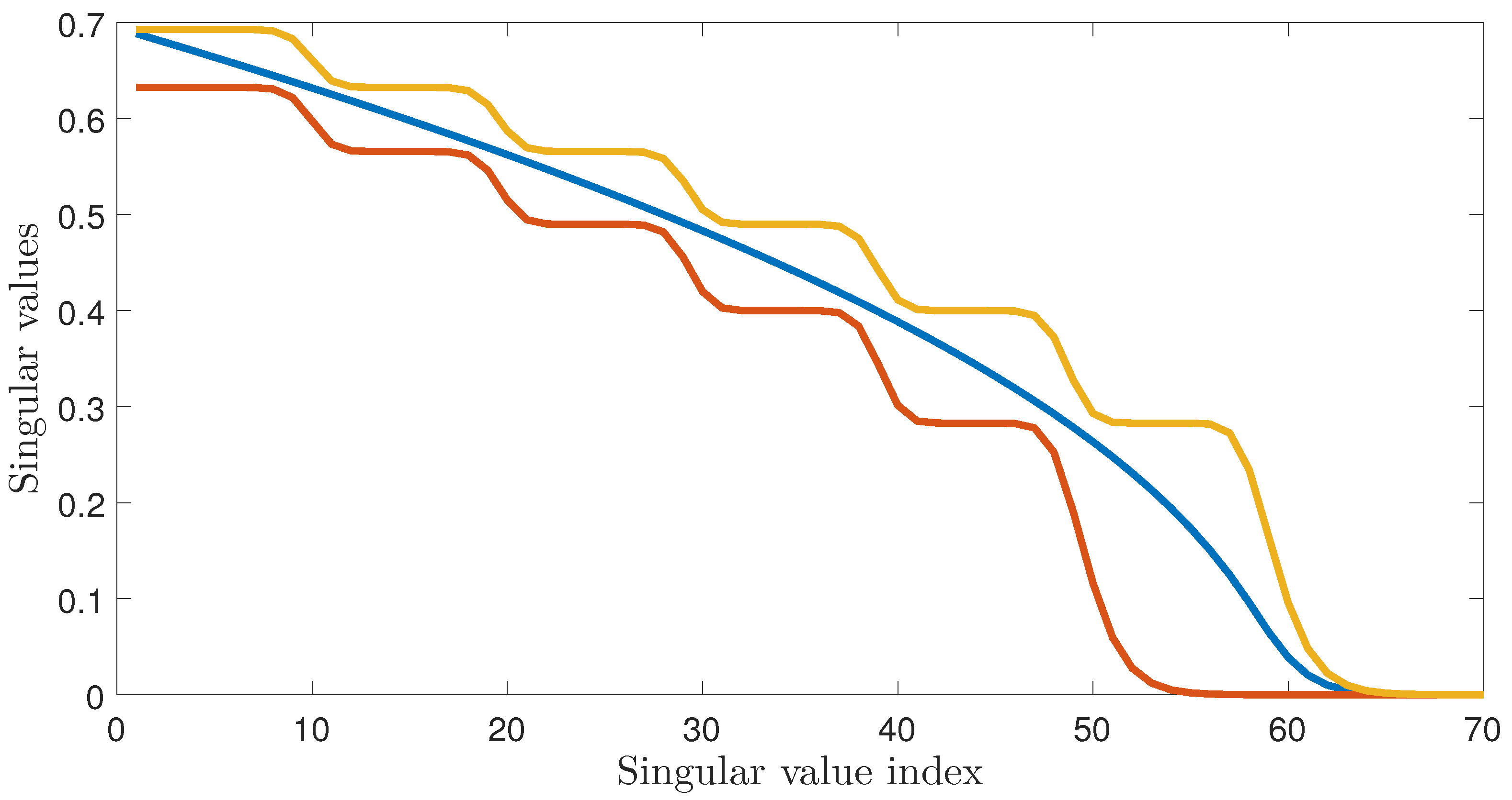
In Figure 5, it can be appreciated that the singular values of the operator ${\mathcal{A}}_i$ are bounded by $\sqrt{{\lambda }_n[\widetilde{{\mathcal{A}}_i^{†}{\mathcal{A}}_i}]}$ and $\sqrt{{\lambda }_n[\widehat{{\mathcal{A}}_i^{†}{\mathcal{A}}_i}]}$, which show a M and $M-1$ step-like behaviour. Moreover, if we choose a noise threshold $\sqrt{{\tau }_{th}}=0.42$ the number of relevant singular values above this threshold is 36, whereas the lower and upper bounds foreseen by Equation (25) are 28 and 38, respectively.

Obviously, by increasing M, the range bounding the effective relevant singular values becomes narrower and the estimation of their number improves. Finally, we can notice that also in the continuous case adding more views simply shapes the singular value behaviour.

3.2. Frequency Diversity

In this section we consider the impact of the frequency diversity on the singular values of the scattering operator. Hence, we suppose to collect the scattering field for a fixed incidence direction (for the sake of simplicity, $x_i=0$) by varying the illumination frequency within the interval $S_k=[k_{min},k_{max}]$. Accordingly, the scattering operator is

$${\mathcal{A}}_f:\chi \left(x\right)\in {\mathcal{L}}_I^2⟶E_S(x_o,k)=\frac{1}{z^{\prime }}{\int }_{-a}^a{e}^{-j(2k{z}^{\prime }+\frac{k}{2z^{\prime }}{(x_o-x^{\prime })}^2+\frac{k}{2z^{\prime }}{x}^{\prime 2})}\chi (x^{\prime })d{x}^{\prime }\in {\mathcal{L}}_{(O\times S_k)}^2.$$

(26)

As in Section 3.1, at first assume that $S_k$ is a discrete set consisting of M uniformly spaced frequencies $k_1=k_{min},k_2=k_{min}+\Delta ,\dots ,k_M=k_{max}$, belonging to the interval $[k_{min},k_{max}]$ and spaced of $\Delta =\frac{(k_{max}-k_{min})}{(M-1)}$. Accordingly, the operator ${\mathcal{A}}_f^{†}{\mathcal{A}}_f$ can be written as

$${\mathcal{A}}_f^{†}{\mathcal{A}}_f{u}_n=\frac{1}{z^{\prime }}\sum _{m=1}^M\frac{2\pi }{k_m}{\mathcal{T}}_{k_m}^{†}{\mathcal{P}}_I{\mathcal{B}}_{{\mathsf{\Omega }}_m}{\mathcal{P}}_I{\mathcal{T}}_{k_m}{u}_{fn}$$

(27)

where now ${\mathsf{\Omega }}_m=[-\frac{k_m{X}_o}{z^{\prime }},\frac{k_m{X}_o}{z^{\prime }}]$. On the contrary, as before, the presence of the operator ${\mathcal{T}}_{k_m}$ can affect the eigenvalues of ${\mathcal{A}}_f^{†}{\mathcal{A}}_f$ because it introduces a modulating term that can change the way in which the bands ${\mathsf{\Omega }}_m$ overlap. To describe the effect of such a modulating term, we can do the following approximation

$$e^{j\frac{k_m}{z^{\prime }}(x^2-y^2)}=e^{j\frac{k_m}{z^{\prime }}(x+y)(x-y)}\approx e^{j\frac{k_m}{z^{\prime }}a(x-y)}$$

(28)

Posing $x+y=a$ is equivalent to choosing the intermediate frequency of modulation [31]. Accordingly, this term translates the frequency band ${\mathsf{\Omega }}_m$ of a $\frac{k_m}{z^{\prime }}a$ factor. It is evident that, if $X_0>a$, such translation does not change the way in which the bands ${\mathsf{\Omega }}_m$ overlap and the effect of such a modulating term is only to introduce a phase factor over the eigenfunctions. Conveniently, Equation (27) can be recast as

$${\mathcal{A}}_f^{†}{\mathcal{A}}_f{u}_{fn}=\frac{2\pi }{z^{\prime }}\sum _{m=1}^M\frac{1}{k_m}{\mathcal{P}}_I{\mathcal{B}}_{{\mathsf{\Omega }}_1}{\mathcal{P}}_I{u}_{fn}+\sum _{m=1}^{M-1}\frac{2\pi }{z^{\prime }}\sum _{l=m+1}^M\frac{1}{k_{0l}}\left({\mathcal{P}}_I{\mathcal{B}}_{{\tilde{\mathsf{\Omega }}}_m}{\mathcal{P}}_I{u}_{fn}+{\mathcal{P}}_I{\mathcal{B}}_{{\widehat{\mathsf{\Omega }}}_m}{\mathcal{P}}_I{u}_{fn}\right)$$

(29)

where ${\mathsf{\Omega }}_1=[-\frac{k_{min}}{z^{\prime }}(X_o-a),\frac{k_{min}}{z^{\prime }}(X_o+a)]$, ${\tilde{\mathsf{\Omega }}}_m=[\frac{k_{min}}{z^{\prime }}(X_o+a)+(m-1)\Delta \frac{(X_o+a)}{z^{\prime }},\frac{k_{min}}{z^{\prime }}(X_o+a)+m\Delta \frac{(X_o+a)}{z^{\prime }},]$ and ${\widehat{\mathsf{\Omega }}}_m=[-\frac{k_{min}}{z^{\prime }}(X_o-a)-m\Delta \frac{(X_o-a)}{z^{\prime }},-\frac{k_{min}}{z^{\prime }}(X_o-a)-(m-1)\Delta \frac{(X_o-a)}{z^{\prime }}]$ (see Figure 6 for a graphical explanation).

If $\Delta$ is chosen to have $\tilde{c}=\frac{a\Delta (X_o+a)}{2z^{\prime }}\gg 4$, $\widehat{c}=\frac{a\Delta (X_o-a)}{2z^{\prime }}\gg 4$ and $c_1=a\frac{k_{min}}{z^{\prime }}{X}_o\gg 4$, by exploiting the same reasoning as before, the eigenvalues exhibit M steps with knees occurring at $N_m=\frac{2a{k}_{min}{X}_o}{\pi z^{\prime }}+(m-1)\frac{2a\Delta X_o}{\pi z^{\prime }}$, with $m=1,\dots ,M$. On the mth step, the eigenvalues are equal to $\frac{2\pi }{z^{\prime }}{\sum }_{l=m}^M\frac{1}{k_l}$. In Figure 7, an example referred to the case $M=3$ is shown: the expected three steps are evident and there is also an accordance between the theoretical and numerical values of ${\sigma }_n[{\mathcal{A}}_f]$. As a result of the discussion above, if $X_0>a$, we find that the maximum number of significant singular values depends on the highest adopted frequency and using more frequency simply shapes the singular value to have a multistep-like behaviour. If $X_0\le a$, the modulating term affects the way in which the bands ${\mathsf{\Omega }}_m$ overlap and the previous conclusions cannot be deduced. In such a case, the translation term introduces a different shaping on the eigenvalues and also an increasing of the number of significant singular values can be obtained. However, such situation does not have a practical interest because it is always assumed to collect the measures over a domain greater than the investigation one.

By following the same logical steps followed in the previous section, we can address also the case of a continuous interval $S_k$ with the assumption $X_o>a$. Thus, the operator ${\mathcal{A}}_f^{†}{\mathcal{A}}_f$ becomes

$${\mathcal{A}}_f^{†}{\mathcal{A}}_f{u}_{fn}=\frac{2\pi }{z^{\prime }}{\int }_{-a}^a{\int }_{k_{min}}^{k_{max}}\frac{1}{k}{e}^{j\frac{k}{z^{\prime }}(x^2-y^2)}\frac{sin\left[\frac{k}{z^{\prime }}{X}_o(x-y)\right]}{\pi (x-y)}d{k}_0{u}_{fn}\left(y\right)dy$$

(30)

Due to Equation (28), we can re-write Equation (30)

$${\mathcal{A}}_f^{†}{\mathcal{A}}_f{u}_{fn}=\frac{2\pi }{z^{\prime }}{\int }_{-a}^a{\int }_{k_{min}}^{k_{max}}\frac{1}{k}{e}^{j\frac{ka}{z^{\prime }}(x-y)}\frac{sin\left[\frac{k}{z^{\prime }}{X}_o(x-y)\right]}{\pi (x-y)}d{k}_0{u}_{fn}\left(y\right)dy$$

(31)

The Fourier transform of the kernel in Equation (31) is given by

$$K\left(u\right)=\left\{\begin{array}{cc}\frac{2\pi }{z^{\prime }}ln(k_{max}/k_{min})\hfill & |u-k_{min}\frac{a}{z^{\prime }}|\le k_{min}\frac{X_0}{z^{\prime }}\hfill \\ \frac{2\pi }{z^{\prime }}ln(k_{max}\frac{X_0+a}{z^{\prime }}/u)\hfill & k_{min}\frac{X_0+a}{z^{\prime }}\le u\le k_{max}\frac{X_0+a}{z^{\prime }}\hfill \\ \frac{2\pi }{z^{\prime }}ln(k_{max}\frac{X_0-a}{z^{\prime }}/(-u))\hfill & -k_{max}\frac{X_0-a}{z^{\prime }}\le u\le -k_{min}\frac{X_0-a}{z^{\prime }}\hfill \\ 0\hfill & elsewhere.\hfill \end{array}\right.$$

(32)

Suppose discretising the frequency interval $[k_{min},k_{max}]$ as before in M intervals with a step $\Delta$. Accordingly, the two spatial frequency intervals $[k_{min}\frac{X_0+a}{z^{\prime }},k_{max}\frac{X_0+a}{z^{\prime }}]$ and $[-k_{max}\frac{X_0-a}{z^{\prime }},-k_{min}\frac{X_0-a}{z^{\prime }}]$ are divided into M intervals with steps $\Delta \frac{X_0+a}{z^{\prime }}$ and $\Delta \frac{X_0-a}{z^{\prime }}$, respectively. We can construct the two auxiliary operators $\widetilde{{\mathcal{A}}_f^{†}{\mathcal{A}}_f}$ and $\widehat{{\mathcal{A}}_f^{†}{\mathcal{A}}_f}$ by adopting the same strategy as in the previous section. Hence,

$$\widetilde{{\mathcal{A}}_f^{†}{\mathcal{A}}_f}=\frac{2\pi }{z^{\prime }}ln(k_{max}/k_{min}){\mathcal{P}}_I{\mathcal{B}}_{{\mathsf{\Omega }}_1}{\mathcal{P}}_I+\sum _{m=1}^M{\tilde{K}}_m({\mathcal{P}}_I{\mathcal{B}}_{{\tilde{\mathsf{\Omega }}}_m}{\mathcal{P}}_I+{\mathcal{P}}_I{\mathcal{B}}_{{\widehat{\mathsf{\Omega }}}_m}{\mathcal{P}}_I)$$

(33)

and

$$\widehat{{\mathcal{A}}_f^{†}{\mathcal{A}}_f}=\frac{2\pi }{z^{\prime }}ln(k_{max}/k_{min}){\mathcal{P}}_I{\mathcal{B}}_{{\mathsf{\Omega }}_1}{\mathcal{P}}_I+\sum _{m=1}^M{\widehat{K}}_m({\mathcal{P}}_I{\mathcal{B}}_{{\tilde{\mathsf{\Omega }}}_m}{\mathcal{P}}_I+{\mathcal{P}}_I{\mathcal{B}}_{{\widehat{\mathsf{\Omega }}}_m}{\mathcal{P}}_I)$$

(34)

Now, by exploiting the same approach as before, the eigenvalues of $\widetilde{{\mathcal{A}}_f^{†}{\mathcal{A}}_f}$ and $\widehat{{\mathcal{A}}_f^{†}{\mathcal{A}}_f}$ can be foreseen and used to upper and lower bound those of ${\mathcal{A}}_f^{†}{\mathcal{A}}_f$. The way to achieve that is summarised in the following statement.

Statement 2:

Let $N({\tau }_{th},c)=♯({\lambda }_n[{\mathcal{A}}_f^{†}{\mathcal{A}}_f])\ge {\tau }_{th}$ be the number of eigenvalues of ${\mathcal{A}}_f^{†}{\mathcal{A}}_f$ that are greater than ${\tau }_{th}$. For example, $N_0=[2k_{min}\frac{a{X}_0}{z^{\prime }\pi }]$. If $X_o>a$, $\tilde{c},\widehat{c}\gg 1$, and hence $c=k_{max}\frac{a{X}_0}{z^{\prime }}\gg 1$, then it approximately holds that

$$\left\{\begin{array}{cc}N({\tau }_{th},c)\le N_0+(m-1)[2(\tilde{c}+\widehat{c})/\pi ]\hfill & {\tilde{K}}_m<{\tau }_{th} and m\in \{2,\dots ,M\}\hfill \\ N({\tau }_{th},c)\ge N_0+m[2(\tilde{c}+\widehat{c})/\pi ]\hfill & {\tau }_{th}<{\widehat{K}}_m and m\ne M\hfill \\ N({\tau }_{th},c)\simeq [2c/\pi ]\hfill & {\tilde{K}}_M>{\tau }_{th}\hfill \end{array}\right..$$

(35)

Of course, the statement rephrases with ${\sigma }_n[{\mathcal{A}}_f^{†}{\mathcal{A}}_f]$ and $\sqrt{{\tau }_{th}}$ in place of ${\lambda }_n[{\mathcal{A}}_f^{†}{\mathcal{A}}_f]$ and ${\tau }_{th}$ for the singular value decomposition of the multifrequency scattering operator.

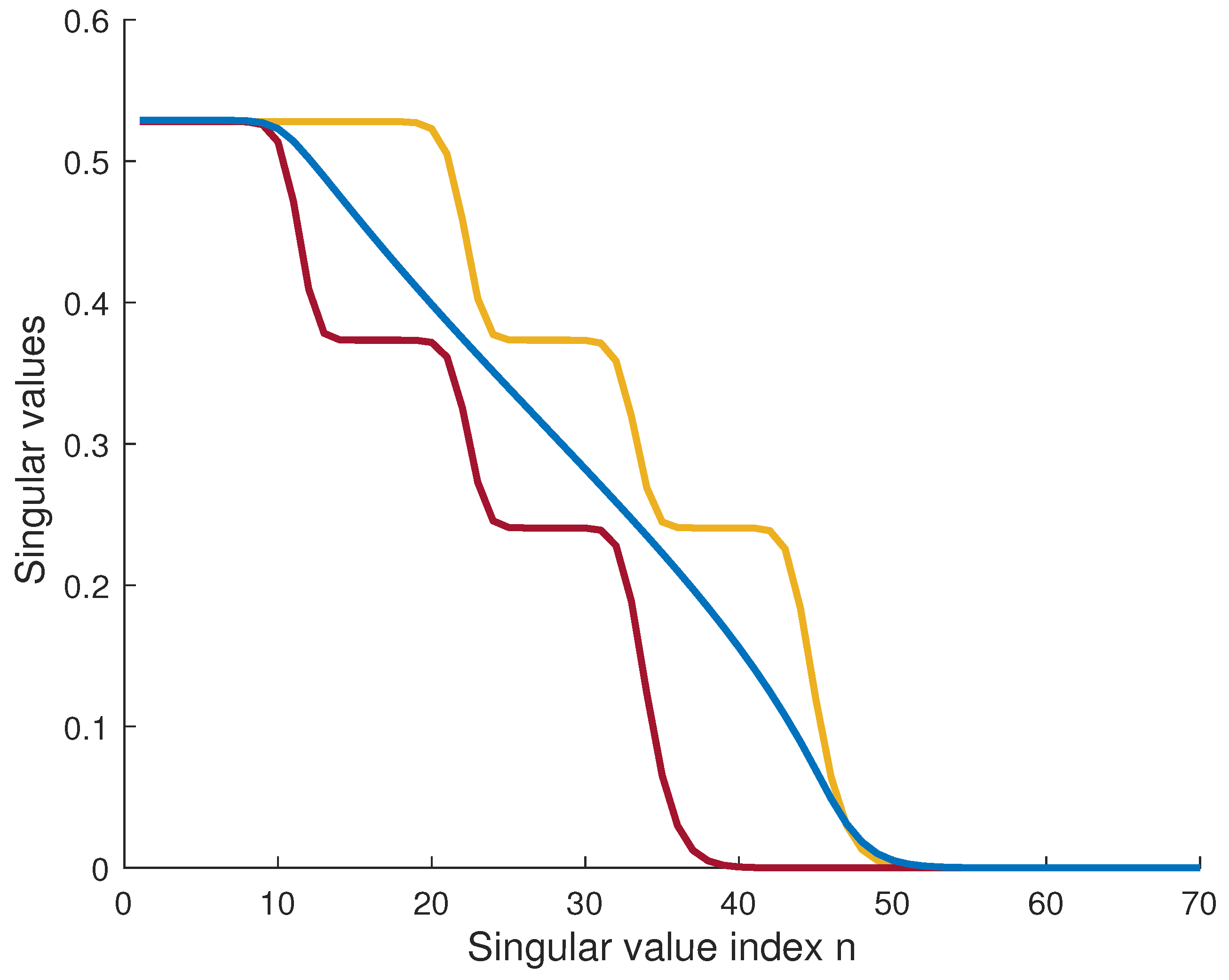
In Figure 8, we show the singular value behaviour of ${\mathcal{A}}_f$ and its bounds. By setting a noise threshold $\sqrt{{\tau }_{th}}$ equal to $0.34$, the number of singular values above this threshold is 24 while the upper and lower bounds estimated with the statement in Equation (35) are 32 and 21, respectively. According to the analysis above, if $X_o>a$, it can be concluded that, to increase the number of significant singular values, the highest adopted frequency should be increased as well. As for view diversity, the use of more frequencies shapes the singular value behaviour by increasing the corresponding numerical values and making the NDF dependent on the tolerable level of noise.

4. Conclusions

In this paper, the role played by the view and frequency diversities on the singular value decomposition of the scattering operator has been analysed. The analysis has been performed by assuming that the observation domain is located in Fresnel zone. The interest in the singular values is due to their link with the metrics (NDF, information content, resolution, etc.) commonly used to assess the performance in linear inverse scattering problems.

Both the cases of discrete and continuously varying incidence directions and frequencies have been addressed. For the discrete cases, the results shown in Section 2 allow obtaining the singular values in closed form and relating their behaviour to the scattering parameters. Instead, for continuous cases, this is not possible. However, a procedure allowing to obtain upper and lower bounds on the singular values behaviour has been introduced. Accordingly, for both diversities, two statements linking the singular values behaviour and the scattering parameters are provided. These can be exploited within imaging applications to properly set the geometrical parameters in order to reach the desired performances.

Under the assumption $X_o>a$, the obtained statements are the same as derived in [4] with the only difference being that the role of variable $u_{max}=sin{\theta }_{max}$ (with ${\theta }_{max}$ the observation angle) is replaced by $\frac{X_0}{z^{\prime }}=tan{\theta }_{max}$. Accordingly, similar conclusions about the role of the illumination diversities can be deduced. In fact, to achieve the maximum number of NDF, two extremal views and the highest adopted frequency are sufficient. By adding views or frequency, we only introduce a shaping on the singular values that makes the NDF noise-dependent. Thus, we can conclude that multiple views and frequencies are redundant. However, adding more views or frequency leads to higher singular values and, hence, to a more stable inversion procedure.

The scenario considered is quite simple but the procedure is general and applicable to more complex scenarios, such as a multi-dimensional case. However, the presented results have been obtained for a specific configuration.

References

- Marks, D.L. A family of approximations spanning the Born and Rytov scattering series. Opt. Express 2006, 14, 8837–8848. [Google Scholar] [CrossRef] [PubMed]
- Tikhonov, A.N.; Arsenine, V.I. Solution to Ill-Posed Problems; Halsted Press: New York, NY, USA, 1977. [Google Scholar]
- Bertero, M.; Boccacci, P. Introduction to Inverse Problems in Imaging; IOP: Bristol, UK, 1998. [Google Scholar]
- Solimene, R.; Maisto, M.A.; Pierri, R. Role of diversity on the singular values of linear scattering operators: the case of strip objects. J. Opt. A 2013, 30, 2266–2272. [Google Scholar] [CrossRef] [PubMed]
- Riesz, F.; Nagy, B. Functional Analysys; Dover: New York, NY, USA, 1990. [Google Scholar]
- Den Dekker, A.J.; Van den Bos, A. Resolution: a survey. J. Opt. A 1997, 14, 547–557. [Google Scholar] [CrossRef]
- Francia, D.; Toraldo, G. Degrees of freedom of an image. J. Opt. A 1969, 59, 799–804. [Google Scholar] [CrossRef]
- Shannon, C.E. A mathematical theory of communication. Bell Syst. Tech. J. 1948, 27, 379–566. [Google Scholar] [CrossRef]
- Kolmogorov, A.N.; Tikhomirov, V.M. ϵ-entropy and ϵ-capacity of sets in function spaces. Am. Math. Soc. Transl. 1961, 17, 277–364. [Google Scholar]
- Raffaele, S.; Maisto, M.A.; Pierri, R. Information Content in Inverse Source with Symmetry and Support Priors. Prog. Electromagn. Res. C 2018, 80, 39–54. [Google Scholar]
- Newsam, G.; Barakat, R. Essential dimension as a well-defined number of degrees of freedom of finiteconvolution operators appearing in optics. J. Opt. Soc. Am. A 1985, 2, 2040–2045. [Google Scholar] [CrossRef]
- Miller, D.A. How complicated must an optical componet be? J. Opt. Soc. Am. A 2013, 30, 238–251. [Google Scholar] [CrossRef] [PubMed]
- Miller, D.A. Communicating with waves between volumes: evaluating orthogonal spatial channels and limits on coupling strengths. App. Opt. 2000, 39, 1681–1699. [Google Scholar] [CrossRef]
- Piestun, R.; Miller, D.A.B. Electromagnetic degrees of freedom of an optical system. J. Opt. Soc. Am. A 2000, 17, 892–902. [Google Scholar] [CrossRef]
- Somaraju, R.; Trumpf, J. Degrees of freedom of a communication channel: Using DOF singular values. IEEE Trans. Inf. Theory 2010, 56, 1560–1573. [Google Scholar] [CrossRef]
- Thaning, A.; Martinsson, P.; Karelin, M.; Friberg, A.T. Limits of diffractive optics by communication modes. J. Opt. A 2003, 5, 153–158. [Google Scholar] [CrossRef]
- Burvall, A.; Martinsson, P.; Friberg, A.T. Communication modes applied to axicons. Opt. Exp. 2004, 12, 377–383. [Google Scholar] [CrossRef]
- Frazin, R.A.; Fischer, D.G.; Carney, P.S. Information content of the near field: Two-dimensional samples. J. Opt. Soc. Am. A 2004, 21, 1050–1057. [Google Scholar] [CrossRef]
- Fischer, D.G.; Frazin, R.A.; Asipauskas, M.; Carney, P.S. Information content of the near field: Three dimensional samples. J. Opt. Soc. Am. A 2011, 28, 296–306. [Google Scholar] [CrossRef] [PubMed]
- Maisto, M.A.; Solimene, R.; Pierri, R. Metric entropy in linear inverse scattering. Adv. Electromagn. 2016, 5, 46–52. [Google Scholar] [CrossRef]
- Magnoli, N.; Viano, G.A. On the eigenfunction expansions associated with Fredholm integral equations of first kind in the presence of noise. J. Math. Anal. Appl. 1996, 197, 188–206. [Google Scholar] [CrossRef]
- De Micheli, E.; Viano, G.A. Metric and probabilistic information associated with Fredholm integral equations of the first kind. J. Int. Eq. Appl. 2002, 14, 283–310. [Google Scholar] [CrossRef]
- Enrico, D.M.; Magnoli, N.; Viano, G.A. On the regularization of Fredholm integral equations of the first kind. SIAM J. Math. Anal. 1998, 29, 855–877. [Google Scholar]
- David, S.; Pollak, H.O. Prolate spheroidal wave functions, Fourier analysis and uncertainty?—I. Bell Syst. Tech. J. 1961, 40, 43–63. [Google Scholar]
- Landau, H.J.; Pollak, H.O. Prolate spheroidal wave functions, Fourier analysis and uncertainty?—II. Bell Syst. Tech. J. 1961, 40, 65–84. [Google Scholar] [CrossRef]
- Raffaele, S.; Pierri, R. Localization of a planar perfect-electric-conducting interface embedded in a half-space. J. Opt. A Pure Appl. Opt. 2005, 8, 10. [Google Scholar]
- Solimene, R.; Mola, C.; Gennarelli, G.; Soldovieri, F. On the singular spectrum of radiation operators in the non-reactive zone: The case of strip sources. J. Opt. 2015, 17, 025605. [Google Scholar] [CrossRef]
- Solimene, R.; Maisto, M.A.; Pierri, R. Inverse scattering in the presence of a reflecting plane. J. Opt. 2015, 18, 025603. [Google Scholar] [CrossRef]
- Gori, F. Integral equations for incoherent imagery. JOSA 1974, 64, 1237–1243. [Google Scholar] [CrossRef]
- Gori, F.; Palma, C. On the eigenvalues of the sinc2 kernel. J. Phys. A Math. Gen. 1975, 8, 1709. [Google Scholar] [CrossRef]
- Solimene, R.; Maisto, M.A.; Romeo, G.; Pierri, R. On the singular spectrum of the radiation operator for multiple and extended observation domains. Int. J. Antennas Propag. 2013, 2013, 585238. [Google Scholar] [CrossRef]
Figure 1.
Geometry of the problem.
Figure 2.
Case of two views . The top panel shows the two frequency bands, while in the bottom panel the singular values of the relative scattering operator are plotted. For the simulation, the configuration parameters are , and .
Figure 3.
Case of three views . The top panel gives a qualitative view of the frequency bands that now overlap. The bottom panel shows the spectrum of the kernel in terms of disjoint bands.
Figure 4.
Singular values behaviour of for views (the other parameters are setted as in Figure 2). The foreseen values for the s on each step are , , and , while for the knees are 14, 28, 43 and 57. They agree with the values indicated in figure.
Figure 5.
Singular values behaviour of for the case of continuous views and (the other parameters are set as in Figure 2). Yellow and red lines represent the square root of the eigenvalues of and , respectively.
Figure 6.
Illustration of how to rearrange the frequency bands to obtain Equation (29) with the assumption .
Figure 7.
Singular values behaviour of for frequencies The configuration parameters are , , , and m. The foreseen values for the on each step are , and , while for the knees are 10, 27 and 43. They agree with the values indicated in figure.
Figure 8.
Singular values behaviour of for the case of continuous frequencies for . The other parameters are set as in Figure 7. Yellow and red lines represent the square root of the eigenvalues of and , respectively.
© 2019 by the authors. Licensee MDPI, Basel, Switzerland. This article is an open access article distributed under the terms and conditions of the Creative Commons Attribution (CC BY) license (http://creativecommons.org/licenses/by/4.0/).
Share and Cite
MDPI and ACS Style
Maisto, M.A.; Munno, F. The Role of Diversity on Linear Scattering Operator: The Case of Strip Scatterers Observed under the Fresnel Approximation. Electronics 2019, 8, 113. https://doi.org/10.3390/electronics8010113
AMA Style
Maisto MA, Munno F. The Role of Diversity on Linear Scattering Operator: The Case of Strip Scatterers Observed under the Fresnel Approximation. Electronics. 2019; 8(1):113. https://doi.org/10.3390/electronics8010113
Chicago/Turabian StyleMaisto, Maria Antonia, and Fortuna Munno. 2019. "The Role of Diversity on Linear Scattering Operator: The Case of Strip Scatterers Observed under the Fresnel Approximation" Electronics 8, no. 1: 113. https://doi.org/10.3390/electronics8010113
Note that from the first issue of 2016, this journal uses article numbers instead of page numbers. See further details here.