A Divisia User Cost Interpretation of the Yield Spread Recession Prediction

1
The Center for Financial Stability, 1120 Avenue of the Americas, 4th Floor, New York, NY 10036, USA
2
Department of Accounting, Economics and Finance, West Texas A&M University, 2501 4th Avenue, Canyon, TX 79016, USA
J. Risk Financial Manag. 2019, 12(1), 7; https://doi.org/10.3390/jrfm12010007
Submission received: 30 November 2018
/
Revised: 28 December 2018
/
Accepted: 30 December 2018
/
Published: 6 January 2019
(This article belongs to the Special Issue Financial Crises, Macroeconomic Management, and Financial Regulation)
Abstract
:A re-evaluation of the role of interest rates is necessary in the wake of the Great Recession. This paper will re-evaluate the interpretation and empirical use of the yield spread as a predictor of recessions, focusing on the simplified methodology in a New York Federal Reserve Bank paper by Estrella and Trubin. Using the user cost difference formula to calculate bond prices following the methodology in the Divisia literature begun by William A. Barnett and a unique data set from the Center for Financial Stability, the yield spread is shown to be a form of the user cost difference, and use of the user cost is shown to marginally improve the predictive abilities of the yield spread. Further research into this view of the link of interest rates and economic activity is proposed.
1. Introduction
In the wake of the 2008–2009 financial crisis and great recession, short term yields pushed down to the zero lower bound. The lack of information produced by the Federal Reserve’s preferred intermediate targets for monetary policy left ambiguity regarding the effectiveness of lower short term interest rates as indicators of monetary easing, while Divisia monetary aggregates demonstrated a clear contraction throughout 2009 and into 2010 (see Barnett et al. (2012) and Belongia and Ireland (2012)). A re-thinking and refocus on the aggregates and their user costs could produce a new perspective and explanation for macroeconomic trends (for example Mattson and Valcarcel (2016) treatment of the compression of the user costs of liquid and non-liquid monetary assets). This paper will take a new look at the relationship between the inverted yield spread and recessions begun by Harvey (1988). The yield spread will be demonstrated be a form of a Divisia user cost difference, which when used as a recession prediction in the same simple manner as Estrella and Trubin (2006) shows improved predictability. Further the interpretation of the inverted difference between the user cost price lends credence to the liquidity preference outcome, and places the yield spread inversion in a more intuitive microeconomic context of supply and demand determining price differences.
The recession predictive abilities of the yield spread have been well established starting in Harvey (1988) and empirically solidified in Estrella and Mishkin (1996) and Estrella and Trubin (2006). It is well established that since the 1970s, once the yield spread drops below 0 that a recession will occur within a year’s time. What is less understood is the reason behind this relationship. An established literature provides a menu of potential explanations such as the segmented markets hypothesis and the expectations hypothesis. More specifically, literature supporting the role of liquidity is well developed starting in Andres et al. (2004), Zagaglia (2013), Canzoneri et al. (2011), and most recently Marzo and Zagaglia (2018), which refer explicitly the substitutability of longer maturity bond assets and more liquid monetary assets as measure of risk preference. This strand of literature points out the key fact that different maturities of bonds can behave as substitutes, using the interest rate difference to price the holding of the bond. This paper will further support that literature in developing the interest difference pricing of these bonds as a “durable service” as is done with monetary assets in the Divsia literature. This allows for a simplified explanation through supply and demand of substitute services of medium of exchange (liquidity) and store of value. This paper will re-interpret the yield spread as an opportunity cost spread of holding a longer term store of value asset over a shorter term medium of exchange (liquid) asset, as used in Barnett (1978, 1980) to develop the Divisia monetary aggregates. This “user cost spread” which demonstrates the current relative price difference between the store-of-value services of bonds will provide the motivation for a recession prediction. The paper will use a simple replication and comparison exercise based on Mishkin and Estrella (1996) and provide an intuitive proof the equivalence of the user cost difference and the yield spread. This is a naïve and simplistic approach to testing the efficacy of the forecast by the user cost spread over the yield spread.
2. Materials and Methods
The methodology for calculating the user cost spread follows the literature begun in Barnett (1978, 1980) and collected in Barnett and Serletis (2005). The benchmark lending rate used by the Center for Financial Stability (CFS) in their calculation of the Divisia monetary aggregate is based on the calculation of the Divisia aggregates in Offenbacher and Kellerman (2013) at the Bank of Israel, as described in Barnett et al. (2012). This lending rate is available by request from the CFS, while other important user cost and monetary aggregate data can be found on their website. Some of the lending rate data can be found outside the CFS resource through the resources described in Barnett et al. (2012).
The ten year and three month yield spread is found through the available data on interest rates provided by the St. Louis Federal Reserve’s Economic Dataset (FRED). These spreads and user costs are compared with the OECD definition of a recession, with the indicator again provided by FRED. The benchmark rate is the same benchmark lending rate selected by the CFS for the calculation of their user costs, which for the 1960s through the 1980s is the upper envelope rate of a basket of various long term rates, the maximum being selected. Since the 1990s, this corresponds to the short term lending rate from the E.2 Survey of Firms provided by the Federal Reserve. Most recently an envelope rate from a basket of available lending rates is used since the discontinuation of the E.2 Survey. The data is monthly observations from January 1968 to September of 2018.
The theory behind the user cost is developed first in Barnett (1978) with roots in Diewert (1974) pricing of durable goods. Following Diewert’s methodology, the durable service of an asset can be priced by the opportunity cost of holding it instead of another benchmark asset; or the difference of the rates of return on these assets relative to the benchmark return. In the Divisia case, monetary assets are durable services, and thus their prices should be measured by a user cost rather than a spot price. The simple equation for calculating the price of holding a monetary asset which provides both the services of a store of value and a medium of exchange (liquidity)at time , with some return , and a benchmark “pure store of value” return (approximated in this case by the short term lending rate), :
which are used as a price in order to determine the expenditure share on each monetary asset within a “liquidity portfolio” of some aggregation level of M1, M2, or M3, which could include extremely liquid forms of monetary assets such as cash, to illiquid forms like overnight repurchase agreements and commercial paper1. For the purposes of this paper we will focus exclusively on the concept of the user cost price, which provides an economic price to the durable service of a means of exchange and store of value that money provides. For the bond markets, it is then argued that they provide two services of liquidity (similar to the medium of exchange service of money) and store of value. As in liquidity premium theory, bonds of different maturities are imperfect substitutes, the elasticities of which are then determined by these user cost prices.
A user cost spread between a ten and two year treasury bond is then defined as the difference:
and note that the user cost of holding on to a shorter term bond is normally larger because the own rate of return of the shorter bond is usually lower than the own rate on the longer term bond. In a similar manner, the yield spread is then the difference between the longer term bond and the shorter term bond, where an inversion represents the signal of a recession in the future:
We then have two signals of price inversion and interest rate inversion to signal the recession, and as will be argued in Section 4, the price inversion intuition is more easily followed than the interest rate inversion.
The user cost spread is used to predict recessions through a logit procedure similar to that outlined in Estrella and Trubin (2006). First, the Estrella and Trubin (2006) method is replicated for the simple probit regression
where is the cumulative normal distribution such that
And is the probability of recession one year ahead in the monthly data.
Those results are then compared with the recession prediction provided by the user cost data. In this case the single variable case is used as in the Estrella and Trubin (2006) case rather than the Mishkin and Estrella (1996) case for simplicity. The methodology can be extended and improved, as is done in the spread literature, by adding control variables for output, equity markets, and other indicators. However, as this paper intends to focus solely on the spreads as signal, we follow the Estrella and Trubin methods.
All estimations are done in R, and the code is provided in Appendix A. R is a free and easily available statistical software program used extensively in academic research and industry. Code is provided for ease of confirmation as well was potential teaching opportunities in Econometrics or Money and Banking courses. Similar programs can be written in SAS, Stata, or Matlab at the discretion of the replicator. With the methodologies firmly established we will move on the results, intuition, and conclusions regarding the interpretation of the yield spread as a user cost difference.
3. Results
The results of the user cost spread and the yield spread provide an improvement in the significance of the prediction using user costs. The normalization of the spread distance using the benchmark rate improves the predictive abilities of the logit model for a recession one year in advance. While this is not a surprising finding given the significance just using the spread, it is noteworthy in that as the spread approaches a zero lower bound, the normalization will allow for better prediction within the binary dependent variable context. The intuitive proof of the normalized equivalence of the user cost spread and the yield spread will be first demonstrated. Then the empirical results of the replication with recent data, and the adjustment to a user cost spread will be compared.
3.1. The User Cost Spread and the Yield Spread
Theorem 1.
The user cost spread of long term and short term bonds is equivalent to the yield spread normalized to the return on a benchmark store of value asset.
This intuitive theorem is easily shown with some algebra, and provides a nice intuitive relationship between the user cost prices of bonds and their rates of return.
Proof of Theorem 1.
For a long term bond denoted and the short term bond denoted is such that , then . By the user cost definition, , and the definition of a yield spread,
such that the spread of the long term and short term bond normalized to the benchmark rate is equal to the spread of the user costs. □
Corollary 1.
If the yield spread is less than zero for some short term bond and some long term bond such that and then the yield spread and the user cost spread are negative, and
The proof of Corollary 1 is trivially true based on the definition of the yield spread and user cost spread. There is then very little intuitive difference in the yield spread and the user cost spread, with a slight comparative advantage for the user cost spread as it is able to normalize the difference in interest rates to the current returns on a pure store of value asset.
3.2. Empirical Results Using the User Cost Spread
The empirical results are provided for both the yield spread and user cost difference in Table 1. Based on the McFadden Pseudo Goodness of Fit and the Akaike Information Criterion, the User Cost difference marginally improves the 10 year and 3 month Treasury Yield Spread. The yield spread predictions line up with the user cost difference predictions, with a marginal difference between the two. The mean absolute error and root mean squared error of an in-sample forecast in lower when using the user cost spread. The sample was split into a 500 observation in sample forecast and 109 observation out of sample forecast with a similar result of lower forecast errors using the user cost differences. The user cost spread provides a more stable recession predictor than the interest rate spreads on their own.
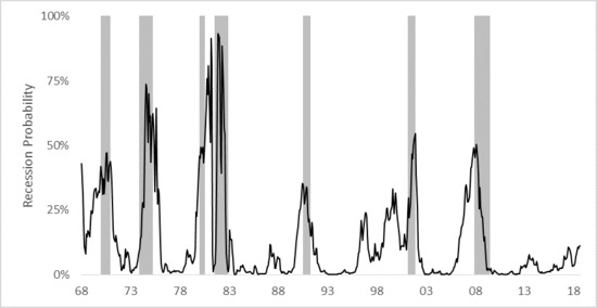
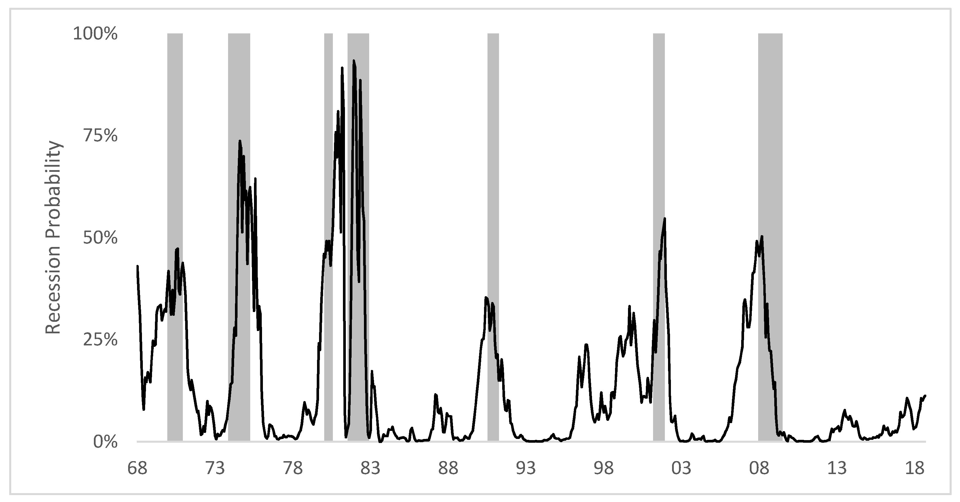
Figure 1 graphs the twelve month advanced recession predictions similar to those in Estrella and Trubin (2006) are demonstrated in Figure 1, showing the prediction probabilities based on the user cost difference rising before the gray recession bar indicators. This is similar to Estrella and Trubin (2006)’s “Figure 2”, with the recession probabilities decreasing in magnitude. While similar, there is a missing bit of information in Estrella and Trubin’s approach, which is this benchmark rate of return in the denominator. The yield spread may be picking up the right recession signals in the decreasing difference of the long and short term yields, but it lacks a relative comparison of these yields to a pure store of value type asset. Both methods stumbled in the 1990s with an increased recession probability predicted, but no recession between 1995 and 1999. Indeed comparing the in-sample and out of sample predictions does not provide a large improvement, however it also does not fare any worse. The similarities between the empirical results confirms the utility of the user cost difference, despite its marginal improvement by including the normalization in the numerator. There is some improvement and no deterioration in forecasting with the user cost spread. The proceeding section will discuss the intuitive reasons for using the user cost over the interest rates.
4. Discussion
In the case of a user cost spread, the relative price of holding on to short term assets for liquidity and store of value purposes is exceeded by the long term asset prices for store of value and liquidity of assets. Consider a normal case where the user cost price of holding on to a short term asset is the store of value return given up of not holding on to the longer maturity asset. In the case of a negative user cost difference, the long term asset provides no premium return over the short term asset. Relative to a pure store of value benchmark represented by the long term asset is a liability compared to holding the short term asset. The price inflection then signals that holding the short term asset with its liquidity provision is preferable to holding the long term asset with its store of value option, indicating the potential for poor economic conditions in the future.
This can be interpreted in the simple microeconomic framework for substitute goods. If the demand for the store of value service drops, the demand for its substitute with more medium of exchange and less store of value rises. In the case of an inflection, the demand for store of value is decreasing at such a rate that the liquidity service cost of holding short term substitutes signaling a preference by holders of these assets for the short term ability to unload assets if necessary. Such an environment would be described as recessionary, with bondholders “unfreezing” the locked in future value for potential present spending power. As conditions improve, holders would then convert their present spending back to the less liquid store of value state provided by longer term bonds. Such an interpretation through the user cost price of holding a long term versus a short term asset would unify what Estrella and Trubin refer to as the “multiplicity of channels” that explain why the spread is related to recessions, into that previously elusive and simple explanation of quantity and price changes among substitute services provided by the assets.
Further the normalization of the interest rate difference to a benchmark rate is important. At the current time period, the pure store of value return is scaling the spread relative to what investors observe at time t, rather than their expectations of future value. The pricing of holding the long term versus short term bond is contained to observed variables in the present time period, rather than determined by an estimated future expectation. If the short term interest rate within the yield spread and user cost spread calculations are potentially a reelection of monetary easing as proposed by Estrella and Trubin (2006), then the normalizing effect of the benchmark rate and the long term rate are the effects of the private markets. For example a monetary tightening that raises interest rates may not be met with an accommodating rise in lending rates and long term bond rates, driving the spreads (user cost and yield) closer to the zero or inversion.
In addition to the availability of observable data at time , the Divisia user cost interpretation provides a “durable service” view on bonds, incorporating both their liquidity service in the short run and their store of value service in the long run. The Divisia monetary aggregate methodology, fully developed in Barnett and Serletis (2005), and empirically utilized in papers such as Anderson, Jones, and Nesmith (1997), Barnett et al. (2012), and Belongia and Ireland (2014), can be extended to the bond markets in their ability to produce a durable liquidity and store of value within the same vein as the analysis of monetary assets like deposits and cash. This user cost approach is well defined within the durable goods literature starting in Diewert (1974), in which the service flow of a durable good is priced within its user cost based on rates of return.
The above interpretation places this discussion firmly in the segmented markets hypothesis groundwork for the predictive effects of term structure on macroeconomic activity. Zagaglia (2013) and Marzo and Zagaglia (2018) for example analyze the cost of bond transaction services and analyzing the liquidity service of bonds. In this context, the interest rate spread is a key measure of risk preference. This research is based on Andres et al. (2004), which outlines imperfect substitution among assets a la Tobin (1969). The Divisia user cost literature shares a heritage with this approach in separating out monetary assets like currency, savings, and money market mutual funds (which are treated as perfect substitutes in the textbook M1 and M2 simple sum measures) as imperfect substitutes. The yield spread, and its similarity to the user cost difference of holdings between short term and long term assets is influenced by the relative holdings of different varieties of bonds. This difference captures changes in aggregate demand and monetary policy which may not be reflected in other macroeconomic indicators, contributing to the predictive nature of the yield spread on macroeconomic activity. However, as Barnett et al. (2012) in terms of constructing monetary aggregates and Barnett (1980) in terms of statistical and index theory point out, it is important for measurement to “get it right”. Placing the yield spread in the context of a user cost price of the durable service of financial assets provides a firmer theoretical foundation for explaining the link.
This interpretation could potentially be expanded to the spreads between corporate bonds and government bonds, or equities. The methodology could be expanded to international cases as the Divisia user cost is normalized by the present benchmark rate of return. If we consider the absolute difference between long term and short term US bonds, then that has little relative comparison to China. However, if the differences between long and short term bonds for both China and the US are normalized to a benchmark loan rate in each country which can provide a starting point for comparison. The potential for empirical and theoretical research using the Divisia user cost interpretation is fertile ground for revisiting previously ambiguous results and expanding comparisons in other contexts.
5. Conclusions
The purpose of the paper is to re-examine the summary empirical analysis of Estrella and Trubin (2006) to a Divisia user cost interpretation. By considering the spread as part of a user cost of the store of value service of differing maturity bonds, the relationship between the inversion of price differences and recessions can be explained by supply and demand behavior among substitutes. Further, the use of the user cost formulation marginally improves the forecast in the univariate regression case. Further research into this interpretation is needed to link the user cost and yield spread relationship with a functional from as in Barnett (1980), and control for other macroeconomic variables that could improve the empirical forecast as in Estrella and Mishkin (1996).
This interpretation is inspired by the long duration of short term interest rates at the zero lower bound in the wake of the Great Recession. Since the 1980s and 1990s, the focus on interest rate changes as a leading indicator has sidelined the more fundamental analysis of the supply of liquidity and store of value available in the economy (the analysis of money). A selection of vibrant literature has re-surfaced with the availability of the CFS Divisia data and research into the superior results from using Divisia monetary aggregates, which can be expanded into also describing the store of value and liquidity services provided by the bond market. In the wake of the Great Recession, a re-evaluation of interest rate relationships with macroeconomic indicators is necessary and powerful. I believe that the Divisia interpretation from the monetary aggregate literature can pair successfully with the segmented markets literature of Andres et al. (2004) which focuses on the relationship between aggregate demand measures, imperfect substitutions, and the yield spread.
Funding
This research received no external funding.
Acknowledgments
Thank you to two anonymous referees for their valuable input and suggestions. Thank you as well to Biyan Tang for her critiques and suggestions.
Conflicts of Interest
The author declares no conflict of interest and has received no outside funding or grants for this research.
Appendix A. Code
The following R Code was used with the spread data. The packages installed and used precede the code, comments are insert with “##”. The table in Table 1 can be generated using the stargazer program for R. The estimates were used to generate Figure 1 in Excel rather than R.
##Installing and loading the necessary packages.
install.packages(“AER”)
install.packages(“stargazer”)
install.packages(“DescTools”)
library(“AER”)
library(“stargazer”)
require(“lattice”)
library(ggplot2)
library(plotly)
library(DescTools)
## Read the CSV file of the spread data.
spread <- read.csv(file=“Location of Data Set”)
## Probit models.
probits <- glm(r ~ s, data=spread, family=binomial(link=“probit”))
summary(probits)
probitu <- glm(r ~ u, data=spread, family=binomial(link=“probit”))
summary(probitu)
## Generates the Pseudo R2 measure.
PseudoR2(probits)
PseudoR2(probitu)
## In sample and out of sample forecasts.
probitsin <- glm(r ~ s, data=spread [1:500,], family=binomial(link=“probit”))
probitsout <- predict(probitsin,newdata=spread[5 01:609,],type=“response”)
residouts <- spread$r[501:609]-probitsout
probituin <- glm(r ~ u, data=spread[1:500,], family=binomial(link=“probit”))
probituout <- predict(probituin,newdata=spread[501:609,],type=“response”)
residoutu <- spread$r[501:609]-probituout
accuracy(probituout, spread$r[501:609])
accuracy(probitsout, spread$r[501:609])
## Generates a stargazer table with the comparison of the spreads.
## Note in the “add.lines” command that the McFadden Pseudo R squared
## value is determined as “0.3111” and “0.3163”. These come from the lines
## of code above that generated the Pseudo R squared in R; I am manually
## inputting them into the stargazer table. Similarly the mean absolute errors
## and root mean squared errors are put in using “add.lines”.
stargazer(probits, probitu,
type=“html”, dep.var.labels = “Probability of Recession”,
covariate.labels=c(“Treasury Spread”,”User Cost Spread”),
add.lines = list(c(“McFadden Pseudo R”, “0.3111”, “03163”),
c(“In Sample MAE”, “0.1684”, “0.1678”),
c(“In Sample RMSE”, “0.2908”, “0.2899”),
c(“Out of Sample MAE”, “0.0430”, “0.0364”),
c(“Out of Sample RMSE”, “0.0562”, “0.0494”),
out=“mishkin.htm”)
References
- Andres, Javier, J. David Lopez-Salido, and Edward Nelson. 2004. Tobin’s Imperfect Asset Substitution in optimizing General Equilibrium. Journal of Money, Credit, and Banking 36: 665–90. [Google Scholar] [CrossRef]
- Barnett, William A. 1978. The User Cost of Money. Economics Letters 1: 145–49. [Google Scholar] [CrossRef]
- Barnett, William A. 1980. Economic Monetary Aggregates. Journal of Econometrics 14: 11–48. [Google Scholar] [CrossRef]
- Barnett, William A., and Apostolis Serletis. 2005. The Theory of Monetary Aggregation. North Holland: Elsevier, ISBN 0-444-50119-3. [Google Scholar]
- Barnett, William A., Jia Liu, Ryan S. Mattson, and Jeff van den Noort. 2012. The New CFS Divisia Monetary Aggregates: Design, Construction, and Data Sources. Open Economies Review 24: 125–45. [Google Scholar] [CrossRef]
- Belongia, Michael T., and Peter N. Ireland. 2012. Interest Rates and Money in the Measurement of Monetary Policy. Journal of Business and Economic Statistics 33: 255–69. [Google Scholar] [CrossRef]
- Canzoneri, Matthew B., Robert Cumby, Behzad Diba, and DavidLópez-Salido. 2011. The Role of Liquid Government Bonds in the Great Transformation of American Monetary Policy. Journal of Economic Dynamics and Control 35: 282–94. [Google Scholar] [CrossRef]
- Diewert, Walter E. 1974. Intertemporal Consumer Theory and the Demand for Durables. Journal of Econometrics 14: 11–48. [Google Scholar] [CrossRef]
- Estrella, Arturo, and Frederic S. Mishkin. 1996. The Yield Curve as a Predictor of US Recessions. Federal Resrve Bank of New York. Current Issues in Economics and Finance 2. [Google Scholar] [CrossRef]
- Estrella, Arturo, and Mary R. Trubin. 2006. The Yield Curve as a Leading Indicator: Some Practical Issues. Federal Reserve Bank of New York. Current Issues in Economics and Finance 12: 5. [Google Scholar]
- Harvey, Campbell R. 1988. The Real Term Structure and Consumption Growth. Journal of Financial Economics 22: 305–33. [Google Scholar] [CrossRef]
- Marzo, Massimiliano, and Paolo Zagaglia. 2018. Macroeconomic Stability in a Model with Bond Transaction Services. International Journal of Financial Studies 6: 27. [Google Scholar] [CrossRef]
- Mattson, Ryan S., and Victor J. Valcarcel. 2016. Compression in Monetary User Costs in the Aftermath of the Financial Crisis: Implications for the Divisia M4 Monetary Aggregate. Applied Economics Letters 23: 1294–300. [Google Scholar] [CrossRef]
- Offenbacher, Edward A., and Mayaan Kellerman. 2013. Divisia Monetary Aggregates for Israel: Background Note and Metadata. Jerusalem: Bank of Israel Research Department, Monetary/Finance Division. [Google Scholar]
- Tobin, James. 1969. A General Equilibrium Approach to Monetary Theory. Journal of Money Credit and Banking 1: 15–29. [Google Scholar] [CrossRef]
- Zagaglia, Paolo. 2013. Forecasting Long Term Interest Rates with a General Equilibrium Model of the Euro Area: What Role for Liquidity Services of Bonds? Asia Pacific Financial Markets 20: 383–430. [Google Scholar] [CrossRef]
| 1 | The CFS provides up to Divisia M4, which includes short term 3-month Treasury Bills with overnight repurchase agreements, commercial paper, and large denomination time deposits. |
Figure 1.
Probability of Recession Using the User Cost Difference.


Table 1.
R Stargazer Results Table for User Cost and Yield Spread Recession Predictions. MAE refers to Mean Absolute Error and RMSE to Root Mean Squared Error. McFadden Pseudo R refers to the McFadden Pseudo R-squared measure.
Table 1.
R Stargazer Results Table for User Cost and Yield Spread Recession Predictions. MAE refers to Mean Absolute Error and RMSE to Root Mean Squared Error. McFadden Pseudo R refers to the McFadden Pseudo R-squared measure.
| User Cost Spread Recession Probabilities | Dependent Variable: | |
|---|---|---|
| Probability of Recession | ||
| (1) | (2) | |
| Treasury Spread | ||
| User Cost Spread | ||
| Constant | ||
| McFadden Pseudo R | 0.3111 | 0.3163 |
| In Sample MAE | 0.1684 | 0.1678 |
| In Sample RMSE | 0.2908 | 0.2899 |
| Out of Sample MAE | 0.0430 | 0.0364 |
| Out of Sample RMSE | 0.0562 | 0.0494 |
| Observations | 609 | 609 |
| Log Likelihood | −167.046 | −165.776 |
| Akaike Inf. Crit. | 338.093 | 335.553 |
Note: *** p < 0.01.
© 2019 by the author. Licensee MDPI, Basel, Switzerland. This article is an open access article distributed under the terms and conditions of the Creative Commons Attribution (CC BY) license (http://creativecommons.org/licenses/by/4.0/).
Share and Cite
MDPI and ACS Style
Mattson, R.S. A Divisia User Cost Interpretation of the Yield Spread Recession Prediction. J. Risk Financial Manag. 2019, 12, 7. https://doi.org/10.3390/jrfm12010007
AMA Style
Mattson RS. A Divisia User Cost Interpretation of the Yield Spread Recession Prediction. Journal of Risk and Financial Management. 2019; 12(1):7. https://doi.org/10.3390/jrfm12010007
Chicago/Turabian StyleMattson, Ryan S. 2019. "A Divisia User Cost Interpretation of the Yield Spread Recession Prediction" Journal of Risk and Financial Management 12, no. 1: 7. https://doi.org/10.3390/jrfm12010007