MinInversion: A Program for Petrophysical Composition Analysis of Geophysical Well Log Data


Department of Geology & Geophysics, Texas A&M University, College Station, TX 77843, USA
*
Author to whom correspondence should be addressed.
Geosciences 2018, 8(2), 65; https://doi.org/10.3390/geosciences8020065
Submission received: 16 December 2017
/
Revised: 3 February 2018
/
Accepted: 5 February 2018
/
Published: 9 February 2018
Abstract
:Knowledge of the composition (mineral and fluid proportions) of rock formation lithologies is important for petrophysical and rock physics analysis. The mineralogy of a rock formation can be estimated by solving a system of linear equations that relate a class of geophysical log measurements to the petrophysical properties of known minerals and fluids. This method is useful for carbonate rocks with complex mineralogies and a wide range of other lithologies. Although this method of linear inversion for rock composition is well known, there are no interactive, open-source programs for routinely estimating rock mineralogy from standard digital geophysical wireline logs. We present an interactive open-source program, MinInversion, for constructing a balanced system of linear equations from digital geophysical logs and estimating the rock mineralogy as an inverse problem. MinInversion makes use of a library of petrophysical properties that can be easily expanded and modified by the users. MinInversion also provides several options for solving the system of linear equations and executing the linear matrix inversion including least squares, LU-decomposition and Moore-Penrose generalized inverse methods. In addition, MinInversion enables the estimation of the joint probability distributions for constituent minerals and measured porosity. The joint probability distributions are useful for revealing and analyzing depositional or diagenetic composition trends that affect porosity. The program introduces ease and flexibility to the problems of rock formation composition analysis and the study of the effects of rock composition on porosity.
1. Introduction
Geophysical logs are continuous recordings of a geophysical parameter along a borehole. They are routinely used for the lithological identification of rock formation units. Gamma-ray and spontaneous-potential logs are useful to distinguish between shale and sandstone units. A special class of logs that are recorded for porosity estimation are particularly useful in composition analysis of rock formations. Their measurements of bulk density, photoelectric factor, acoustic slowness, and neutron porosity capture the bulk or resultant property of all rock constituents combined. Porosity is a measure of the void space in rocks that is filled with fluids; the fluids are also treated as one of the rock constituents. The relationship between the log measurements and the properties of the mineral and fluid constituents can be modeled using a set of linear equations [1,2] expressed as:
where C is a matrix of the petrophysical properties of the rock constituents, V is a vector of the unknown proportions of the rock constituents and L is a vector of geophysical log measurement which represent the bulk petrophysical properties of the rock formation. An additional unity equation is included which states that the sum of all mineral and fluid proportions is unity. For example, Equation (1) with the predominant components of quartz, calcite, clay and brine and log measurements of sonic travel time, density and photoelectric absorption factor can be written out explicitly as:
where , , , V stand for density, photoelectric factor, sonic travel time and volume fraction respectively, is porosity. The subscripts q, , cl, f and l stand for quartz, calcite, clay, fluid (brine) and log measurement respectively. Equation (1) can be solved using a forward modeling procedure where geological models with different mineral and fluid combinations are used to generate alternate log measurements for comparison to the actual logs [2]. The more useful method for solving Equation (1) is to cast it as an inverse problem and solve for V:
Although the above procedure is well established, there are no interactive open source programs for constructing and solving Equation (1) directly from the digital geophysical logs. Doveton et al. [3] demonstrated the use of an Excel spreadsheet add-on capable of calculating well log composition for defined petrofacies, however the constant modification to Excel spreadsheet functionality means that the spreadsheet add-ons also require constant modification and effort duplication. Other software like PfEFFER-java (Kansas Geological Society, Wichita, KS, USA), Geolog (Paradigm, Houston, TX, USA), PowerLog (CGG, Paris, France), TechLog (Schlumberger Limited, Houston, TX, USA) are capable of estimating lithology composition, however, these programs are not open-source; this significantly limits their use, expansion and modification by users. In addition the methods used by these programs for computing the mineral composition volumes are often not revealed, hence it is difficult to compare the performance of different methods. We present here an interactive open-source program, MinInversion, for constructing a balanced system of linear equations and estimating the rock mineralogy as an inverse problem. The program is open-source and can be easily modified and expanded by users. In addition the program facilitates the comparison of the performance of different inversion methods for composition analysis. The program interactively reads in log files in the standard LAS file format or Excel spread sheet format and provides choices of mineral and fluid constituents from a library of petrophysical properties compiled from several sources (see Table 1). The library of petrophysical properties contains various minerals and composite mineral mixtures and can be easily expanded and modified by the user. The program also provides the options on the method for executing the inversion computation including the least squares, LU-decomposition and the Moore-Penrose generalized inverse methods.
2. Geophysical Log Descriptions
The class of useful logs for rock composition analysis includes porosity logs (sonic, density and neutron logs) and litho-density logs. Sonic logs measure the interval travel time or slowness (inverse of velocity) of a formation as a continuous function of depth. The slowness varies with lithology and porosity. Wyllie’s time averaging equation [4], gives a simple relationship between velocity and porosity:
where is the porosity, is the fluid sonic velocity, is the matrix sonic velocity and is the logged velocity. Wyllie’s equation can be written in terms of slowness as:
where is the interval travel-time of the saturating fluid, is the interval travel-time of the rock matrix, and is the logged interval travel-time. The density logs measures the bulk density of a rock formation as a continuous function of depth. The bulk density is a combination of the densities of mineral and fluid components. It is used to calculate porosity and is good for lithology identification. Equation (6) shows the bulk density log response equation
where is the measured bulk density, is the density of the rock matrix, is the density of the saturating fluid.
Neutron logs are a continuous measurement of the fast neutron bombardment of rock formations as a function of depth. It targets the hydrogen density of the rock volume, which modifies neutrons rapidly; hence it is primarily a measure of the rock formation’s fluid and gas content. It is reported in neutron porosity units and is generally calibrated to a default of equivalent limestone porosity units. On this porosity scale, zero porosity is matched with the mineral calcite and so the equivalent zero reading for other minerals must be used to accommodate other lithologies. The neutron porosity is sensitive to hydrogen in all forms, so that minerals that contain water of crystallization, such as gypsum, register high equivalent neutron porosities which can then be used in the volumetric estimation of these minerals. Equation (7) shows neutron log response equation.
where is the neutron log measurement, is the neutron value of the rock matrix, is the neutron value of the saturating fluid.
The photoelectric log was introduced as a curve on the lithodensity log by Schlumberger, but is now recorded routinely by most logging companies. It measures the photoelectric absorption factor cross-section index of a rock formation, which is defined as , where Z is the average atomic number of the rock constituents. It is useful as a matrix indicator especially if cross-multiplied with the corresponding density value to produce a volumetric-scaled parameter. However, this is closely correlated with the photoelectric factor, so that effective volumetric composition analysis can be made directly from values recorded on LAS files. Use of the photoelectric factor in inversion is limited if the drilling mud used while logging contains barite because the photoelectric absorption index of barite is significantly larger than that of most minerals. Equation (8) shows the photoelectric factor log response equation.
where is the photoelectric factor log measurement, is the photoelectric factor of the rock matrix, is the photoelectric factor of the saturating fluid.
We will use the known petrophysical properties of specific minerals to invert for the proportions of the minerals that sum together to give the actual log measurements at a particular depth. For each depth point within the well or a selected zone, MinInversion automatically constructs the linear system of equations using the log response equations for each log together with the unity equation (which states that the sum of all components is unity) and the above mentioned petrophysical properties. The system of linear equations is then solved using whichever method is currently highlighted in the methods panel of the program. The inversion model used in solving the system of equations has no inherent constraints to prevent negative proportion estimates. If negative proportions occur, they may be used as diagnostic tools for the better choice of mineral components. Other things that could lead to negative proportions are: tool error and adverse borehole environments [2]; it is therefore advisable to check for these problems before using logs in the inversion procedure.
Carbonate rocks in general have more complex mineralogy than siliciclastic rocks hence, inversion for petrophysical properties is most important for carbonate rocks [5]. The method has been used effectively to estimate the complex mineralogy of carbonate rocks in the Permian basin, West Texas [2,5].
3. Software Description
3.1. Linear Inversion Theory
The MinInversion program enables the solving a system of linear equations using any of three methods: least squares inversion, the LU-decomposition and Moore-Penrose generalized inverse methods. A least squares solution for Equation (1) can be found by solving for a particular vector V that minimizes a measure of the misfit between the data L and . Equation (9) shows the residual (r) between L and . The least squares method seeks to minimize the sum of the square of the residuals (r). The normalized least squares solution is expressed in Equation (10).
where C is a matrix of the petrophysical properties of the rock constituents, V is a vector of the unknown proportions of the rock constituents and L is a vector of geophysical log measurement which represent the bulk petrophysical properties of the rock formation. T is the transpose operator.
In LU-decomposition, given that matrix C is non-singular, it is separated or decomposed into a lower triangle matrix () and an upper triangle matrix () using the Gaussian elimination forward elimination steps. Equation (1) is then replaced with two new Equations (11) and (12). The solution is found by solving for W in Equation (11) and then back substituting W in Equation (12).
The Moore-Penrose generalized inverse [6,7], is a generalized inverse method that can be used if the inverse of C does not exist. The pseudo inverse is constructed by finding the set of all vectors () such that the euclidean norm reaches its least possible value. is defined as the unique matrix that satisfies the Equations (13)–(16) and can be computed using singular value decomposition (SVD) [7].
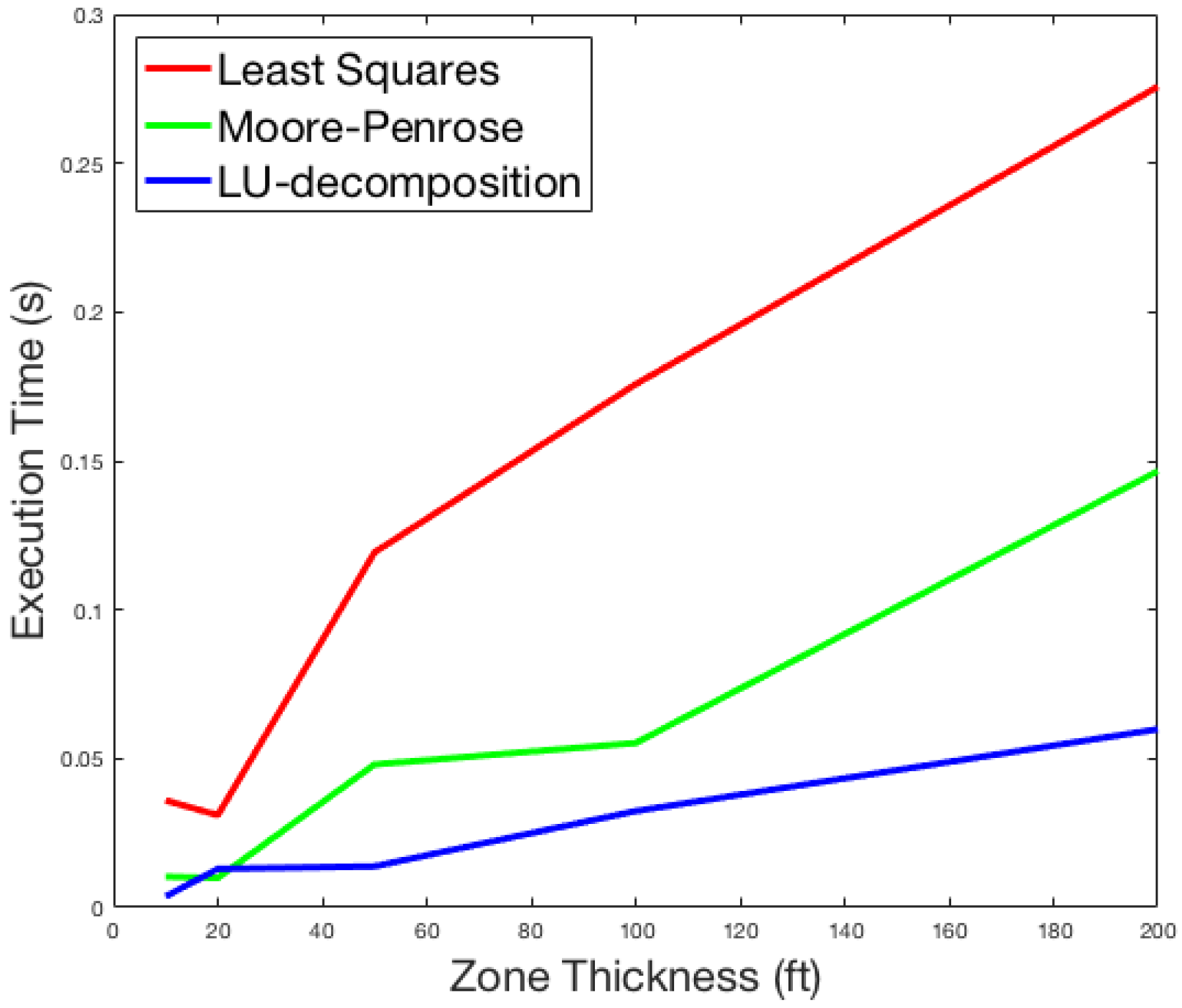
The execution times for the LU-decomposition methods and Moore-Penrose generalized inverse methods are generally smaller than the required execution time of the least squares method, however the LU-decomposition methods and Moore-Penrose generalized inverse methods are not guaranteed to always be stable. Figure 1 shows the execution times for the three methods as a function of well zone thickness.
3.2. Program Usage
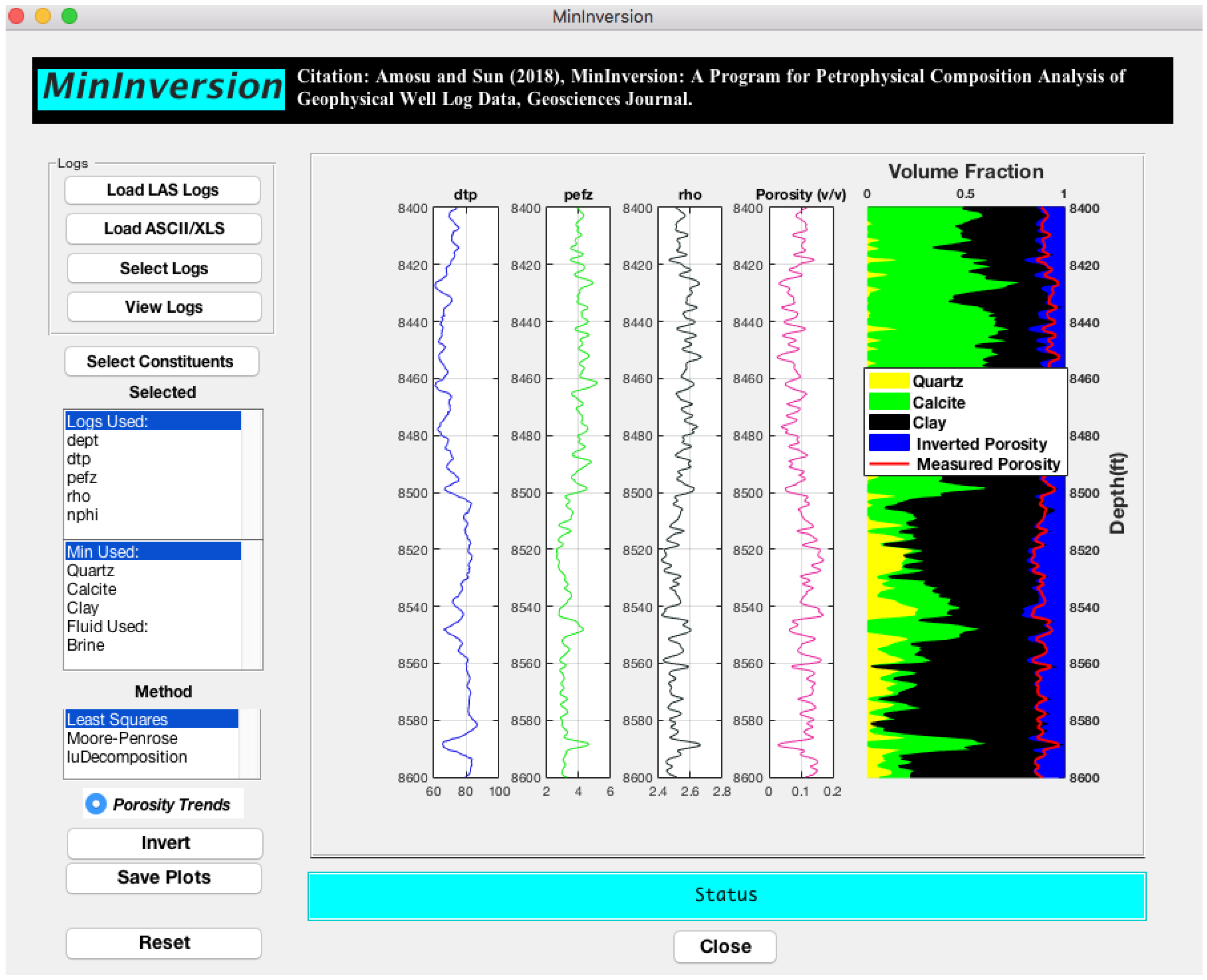
The MinInversion program is written in Matlab and has an interactive graphical user interface (GUI). Figure 2 shows the graphical user interface for the program with an inset example. The program usage is described below:
- Input: The “Load LAS Logs” program allows the user to interactively select geophysical logs in the standard LAS (Log ASCII Standard) file format. The LAS format is a standard file format common in the oil and gas and water well industries for storing well logging data. The “Load ASCII/XLS” button lets the user input geophysical well log data in tabular ascii format, Microsoft Excel or comma-separated-value formats.
- Choosing Logs: After loading the input data, the “Select Logs” button lets the user choose the logs to be used in the inversion and match the selected logs with mnemonics recognized by the program. The selected logs appear in the first panel on the left in the GUI.
- Viewing Logs: The “View Logs” button allows the user to display the selected logs in the program’s main display axes.
- Selecting Rock Constituents: The “Select Constituents” button is used to select the mineral and fluid components with make up the rock. The program suggests the number of components to select based on the number logs available from the previous selection. The constituents are selected from the library of petrophysical properties (which can be easily expanded by the user). The selected constituents appear in the second panel on the left in the GUI. Table 1 shows a section of the library of petrophysical properties.
- Inversion Method: The program currently permits inversion using three methods: least squares, Moore-Penrose generalized inversion and LU-decomposition methods. The “Invert” button calculates a solution to the linear system of equations constructed from the selected logs and constituents using the method selected in the “Method” panel. The results composition volume is then displayed alongside the logs in the main display axes. If the “Porosity Trends” button is toggled on and the porosity logs have been loaded, the program generates plots of joint probability distribution of measured porosity with constituent proportions.
- Other features: The status bar displays the current status of the program during any of the above processes. The “Save plots” generates high resolution images of the logs, the composition volume, a combination plot of logs and composition, and the joint probability distribution plots in a folder labeled “MinInversion_Output” located in the current Matlab folder. The “Reset” button is used to clear the memory and reset the program.
4. Applications and Examples
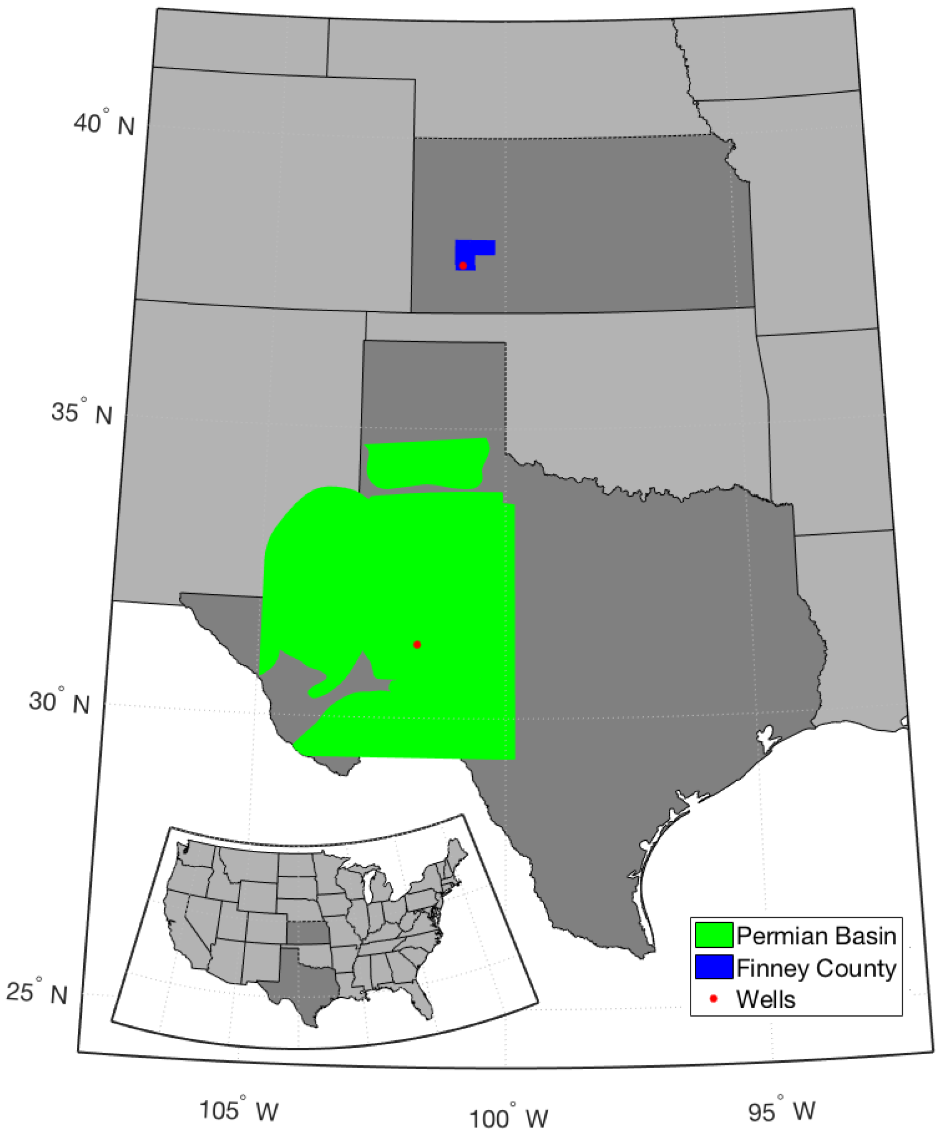
We demonstrate the application and usage of the MinInversion program using geophysical log data from the Permian Basin, West Texas and the Atokan and Cherokee Pennsylvanian sandstone formations, Kansas. Figure 3 shows the location of the wells used in this study.
4.1. Permian Basin, West Texas
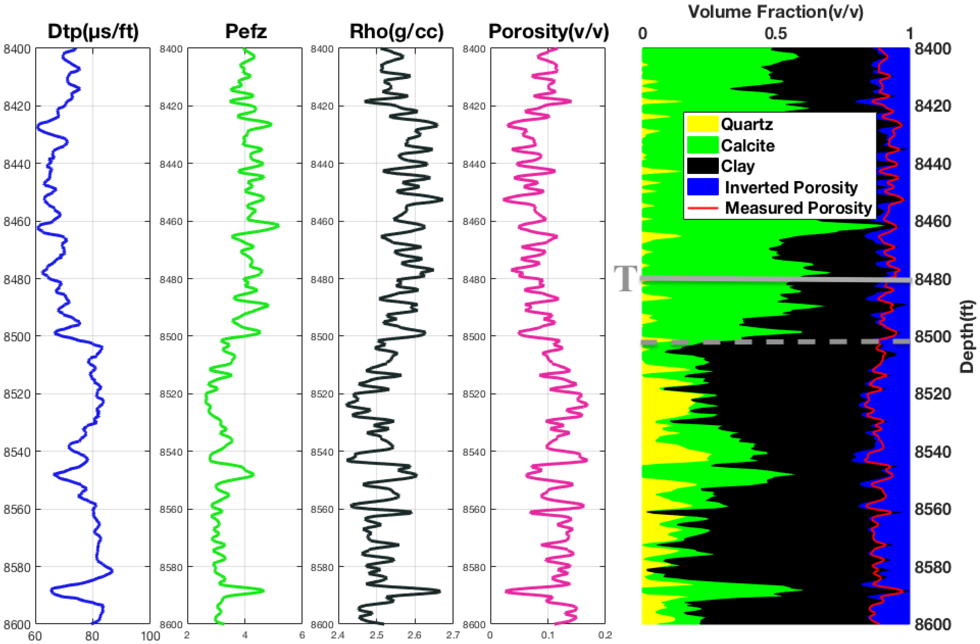
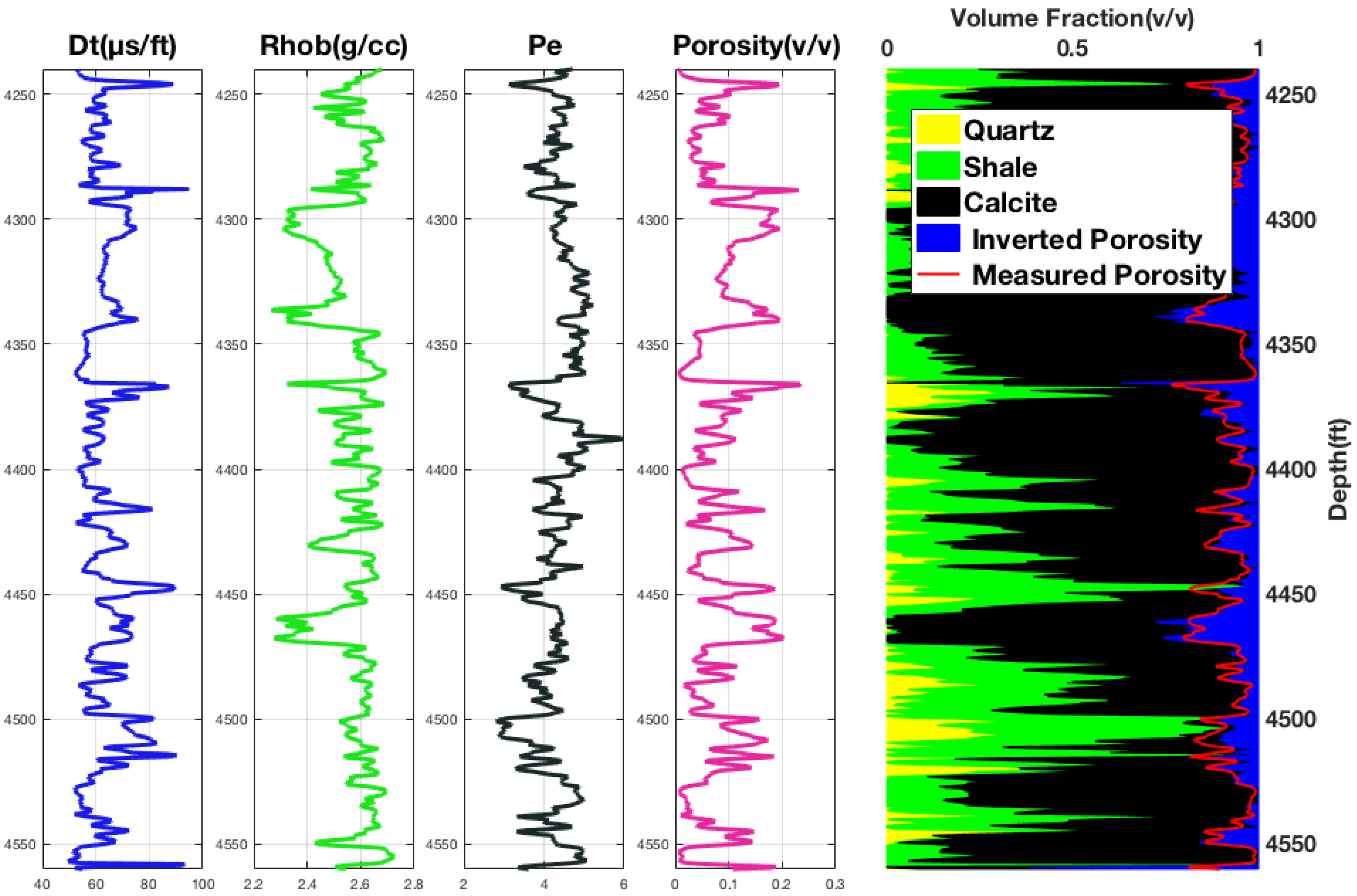
The Permian basin located on the northwestern border of Texas and the southeastern border of New Mexico is one of most prolific oil producing areas onshore of the US. The Permian basin is a foredeep basin that developed during the late Mississippian and early Pennsylvanian [8]. Reservoir rocks of the Wolfcamp carbonate platform, consists of cyclic shallow-water facies affected by diagenesis [9]. X-ray diffraction measurements on sparse core samples reveal that the three predominant components are quartz, calcite and clay. Using MinInversion, we invert for the proportion of the components. Figure 4 shows the results calculated using the least squares method. The inverted porosity (blue) is obtained from the unity equation by subtracting the estimated mineral volumes from unity. A good match can be observed between the inverted and measured porosity (neutron porosity). A division between the quartz rich zone and the calcite rich zone can also be observed (broken line).
4.2. Pennsylvanian Sandstone, Kansas
We apply MinInversion to the late Atokan aged sandstone formation and the early Desmoinesian (Cherokee group), from a well located in Finney County, Kansas. The middle Pennsylvanian sediments are made up of both marine and nonmarine rocks containing mixed clastic sediments, shales and limestone. The amount of limestone is indicative of a increasingly wide spread marine invasion of the area during the middle and later Pennsylvanian time [10]. The Atokan stage consists of dark interbedded cherty limestones and black shales. Gradational contact occurs between Atokan and Desmoinesian rocks in the basinward parts of the Hugoton embayment [11]. The lithofacies of the Cherokee group consists of sandstone, sandy shale and widely extensive carbonate formations interbedded with thinner shale units; the carbonate rocks thicken basinward. We invert for the predominant components of quartz shale and calcite. Figure 5 shows logs used and the composition analysis results computed using the Moore-Penrose generalized inverse method. The inverted porosity (blue) is obtained from the unity equation by subtracting the estimated mineral volumes from unity. A good match can be observed between the inverted and measured porosity (neutron porosity).
4.3. Depositional/Diagenetic Composition Trends
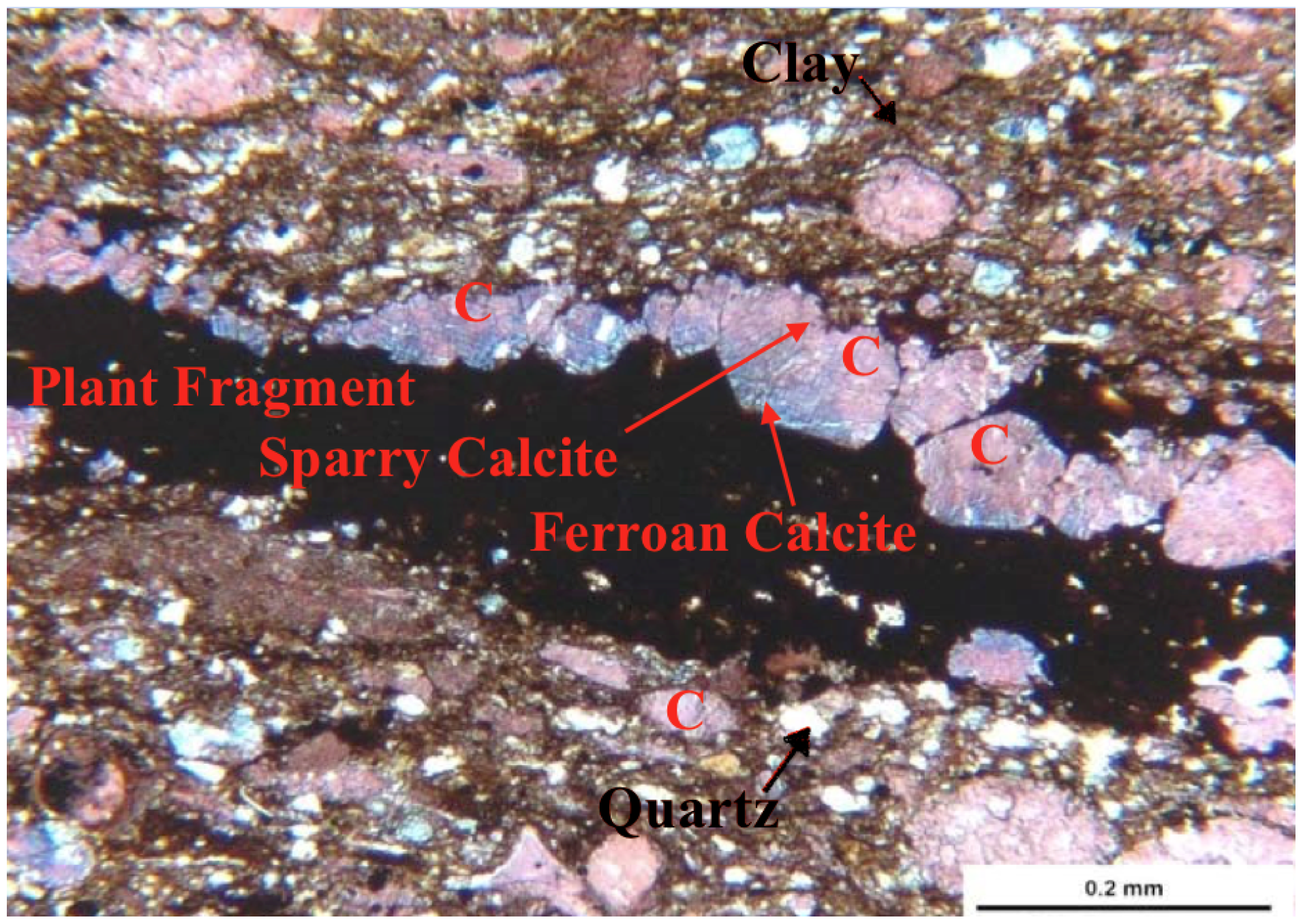
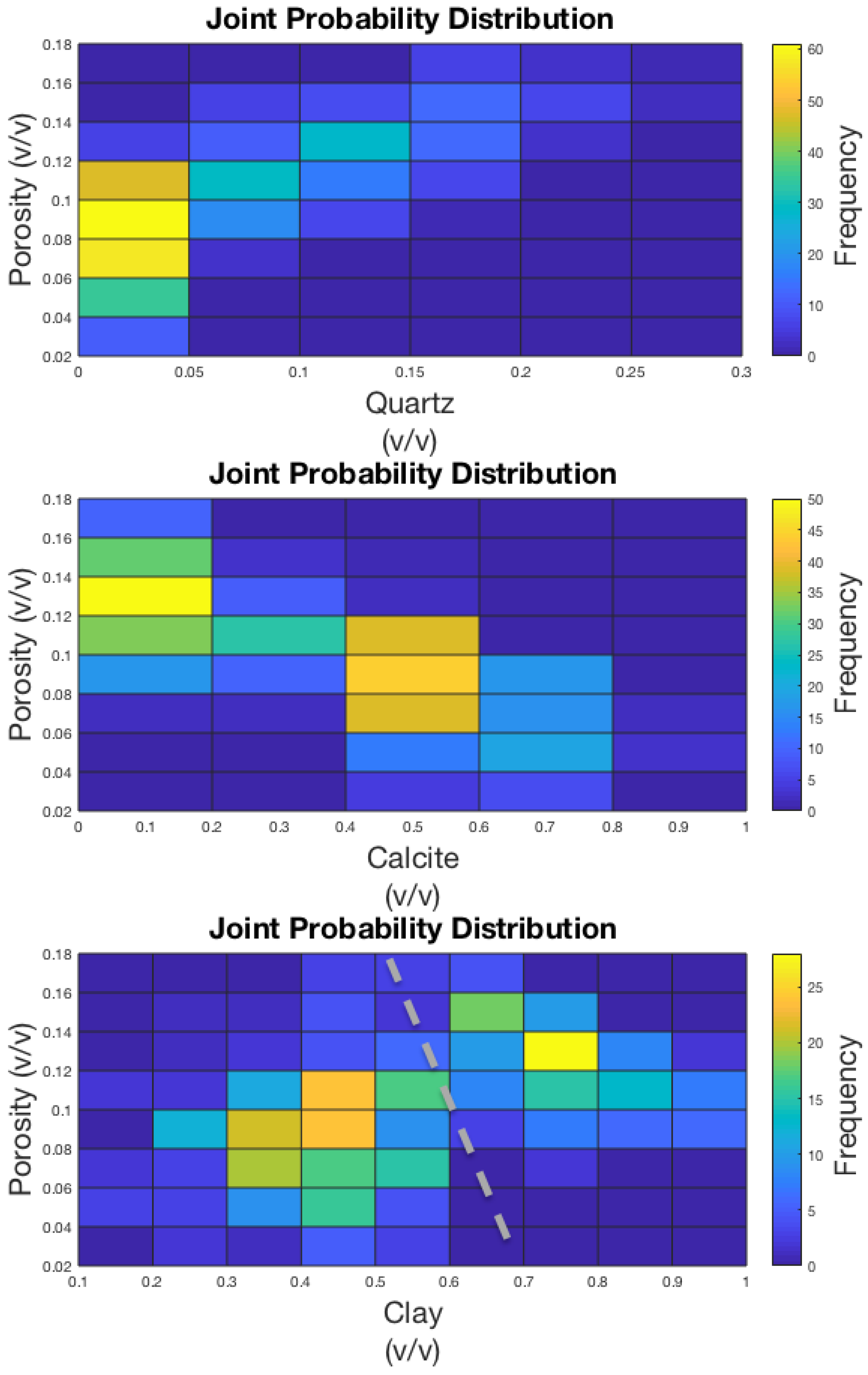
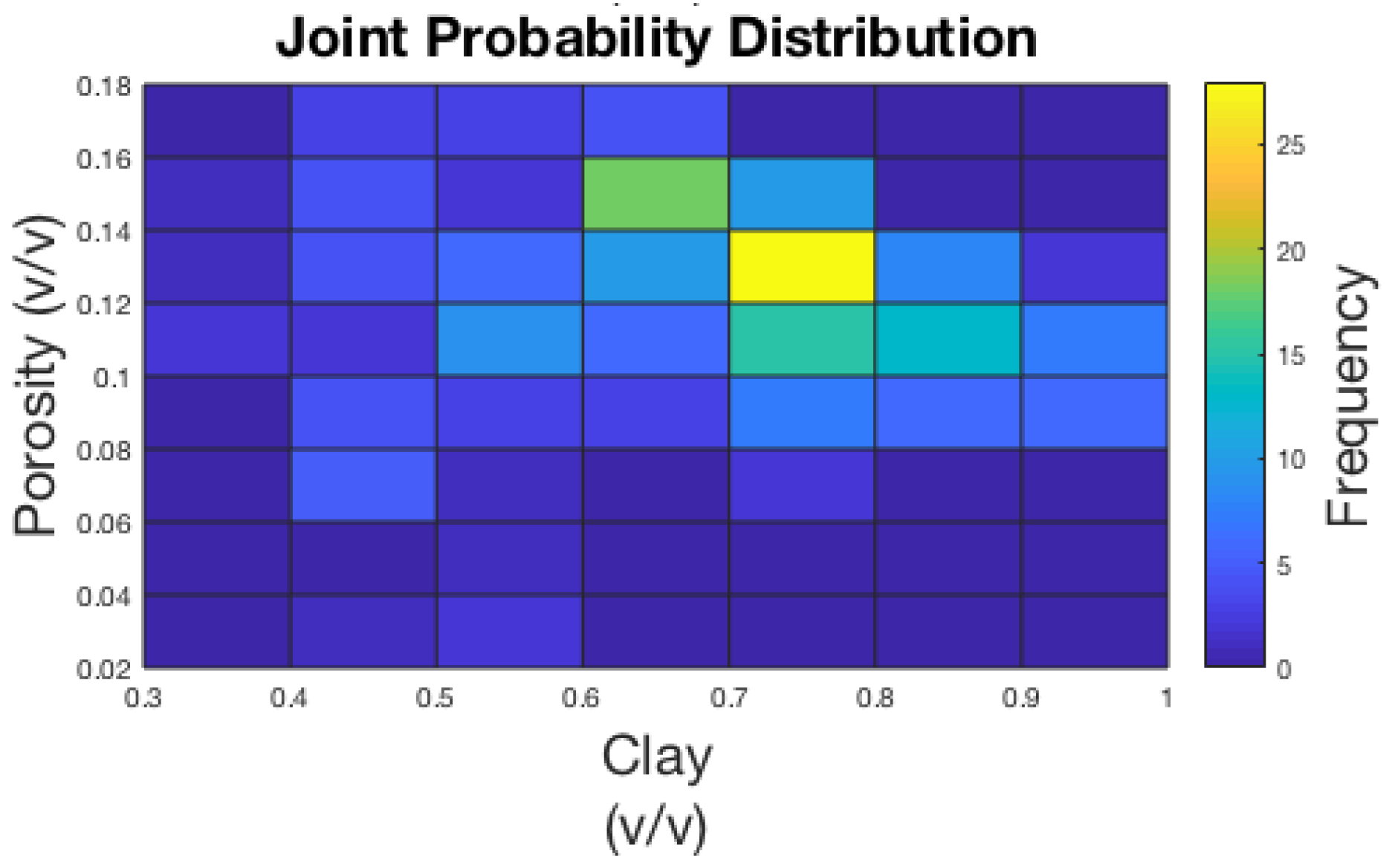
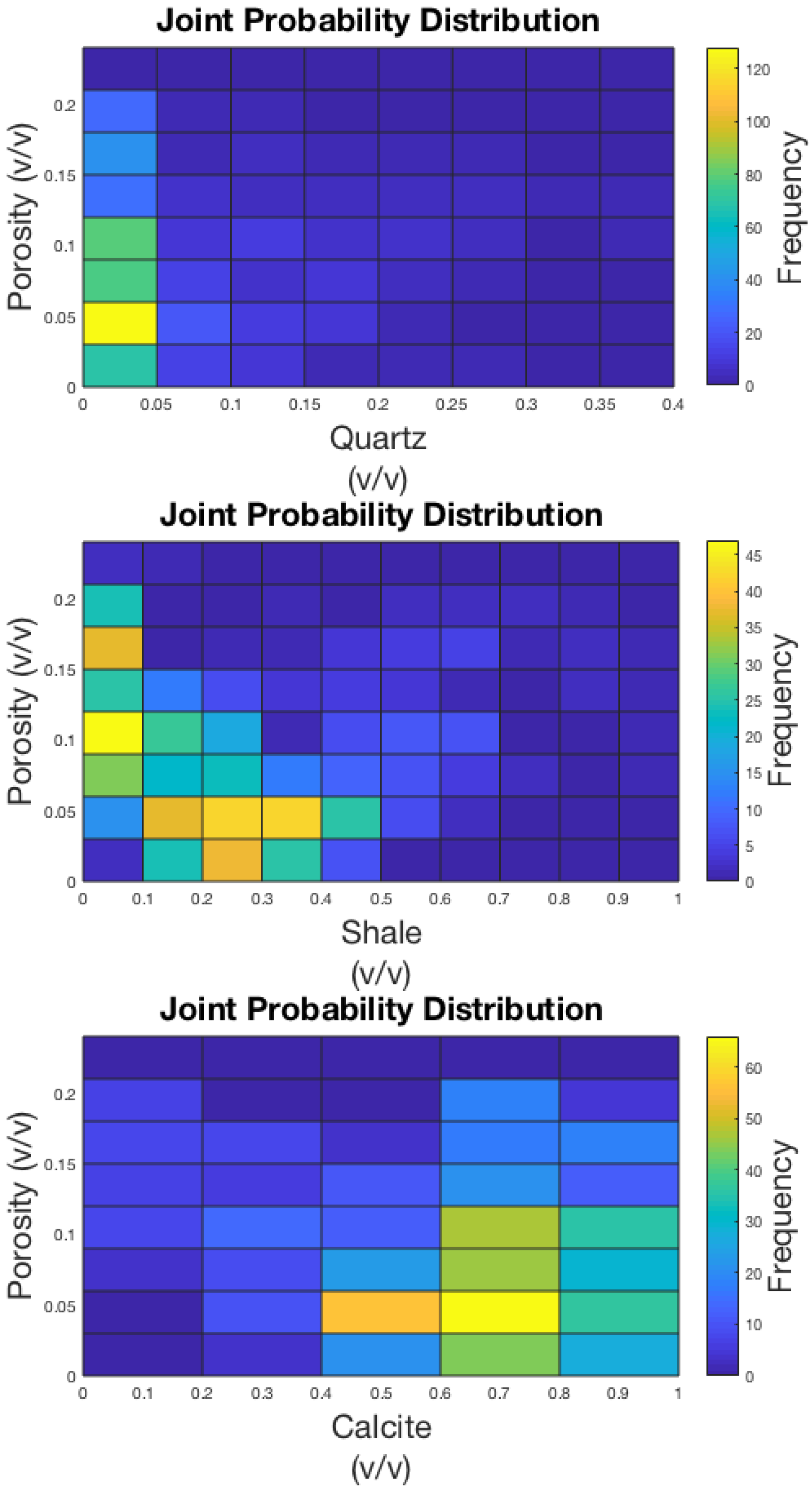
MinInversion can be used to investigate depositional or diagenetic composition trends that affect porosity. Interpretation of composition analysis results can be juxtaposed with other data types such as thin-section photomicrographs and core data. Figure 6 shows thin section photomicrographs obtained from samples corresponding to the location marked T within the well in the Permian Basin (Figure 4). The photomicrographs show by calcite (marked C), Quartz particles and clay; porosity is mainly from microporosity in organic matter and interparticle porosity. Calcite acts as cement and the multiple stages of calcite cementation imply that the calcite cementation is diagenetic. Figure 7 shows the joint probability distribution of measured porosity and rock constituents for the Permian Basin well calculated using MinInversion. An increase in calcite can be observed to correspond to a decrease in porosity indicating the effect of calcite cementation; this is in agreement with the photomicrograph observations. An increase in quartz content can be observed to correspond to an increase in porosity; this is caused by interparticle porosity between the grains. The distribution of clay with porosity reflects differences in the quartz rich and the calcite rich zone (separated with the broken line). We calculate the joint probability of measured porosity and clay for the two zones separately (Figure 8). The calcite rich zone, which has less clay, shows no obvious trend between clay and porosity. The quartz rich zone, which has more clay, shows a decrease in porosity with increasing clay content, indicating clay may be pore-filling. However the quartz rich zone has higher porosity than the calcite rich zone, which reflects a combination of the effect of less calcite cement and more quartz.
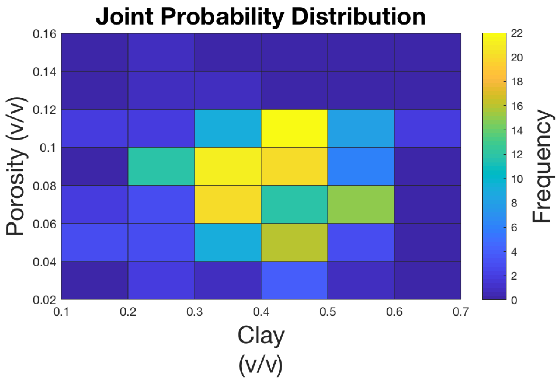
Figure 9 shows the joint probability distribution of measured porosity and rock constituents for a well in the late Atokan and early Desmoinesian deposits of the Pennsylvanian, Kansas. An increase in calcite can be observed to correspond to a decrease in porosity indicating calcite cementation. Quartz content increases with porosity, indicating interparticle porosity, however the data generally has more samples with a smaller proportion of quartz content. An increase in shale content corresponds to a decrease in porosity indicating the high compressibility of shale.
5. Conclusions
We present an interactive open source program for constructing and solving a balanced system of linear equations and estimating the rock mineralogy as an inverse problem. The program interactively reads in log files in the standard LAS file format or excel spread sheet format, provides choices of mineral and fluid constituents from a library of petrophysical properties and constructs a system of linear equations for inversion. The program also provides the options on the method of executing the linear matrix inversion computation including the Least squares, the Moore-Penrose generalized inverse and the LU-decomposition methods. In addition MinInversion facilitates the study of depositional or diagenetic composition trends that affect porosity in the data by generating plots of the joint probability distributions of measured porosity and rock constituents. The program introduces ease and flexibility to the problems of mineral composition analysis and the depositional or diagenetic effects of rock composition on porosity using geophysical logs; this will aid in better decision-making in subsurface resource exploration especially when composition analysis is juxtaposed with other types of data.
Supplementary Materials
The following are available at https://www.mdpi.com/2076-3263/8/2/65/s1. MinInversion Package. The software source code and demonstration video are available online at https://goo.gl/spdwMf.
Acknowledgments
The authors thank the Berg-Hughes Center for Petroleum and Sedimentary systems, the Crisman Institute of Petroleum Engineering and the Kansas Geological Survey for making available the data used in this study.
Author Contributions
Adewale Amosu and Yuefeng Sun developed the code and wrote the paper.
Conflicts of Interest
The authors declare no conflict of interest.
References
- Doveton, J.H.; Cable, H.W. KOALA–Minicomputer Log Analysis System for Geologists. AAPG Bull. 1979, 63, 441. [Google Scholar]
- Doveton, J.H. Compositional Analysis of Mineralogy. In Principles of Mathematical Petrophysics; International Association for Mathematical Geosciences: Houston, TX, USA, 2014; Volume 9, pp. 94–121. [Google Scholar]
- Doveton, J.H.; Guy, W.; Watney, W.L.; Bohling, G.C.; Ullah, S.; Adkins-Heljeson, D. Log Analysis of Petrofacies and Flow-Units with Microcomputer Spreadsheet Software. In Proceedings of the Transactions of the 1995 AAPG Mid-Continent Section Meeting, Oklahoma City, OK, USA, 30 September–3 October 1996. [Google Scholar]
- Wyllie, M.R.J.; Gregory, A.R.; Gardner, L.W. Elastic Wave Velocities in Heterogeneous and Porous Media. Geophysics 1956, 21, 41–70. [Google Scholar] [CrossRef]
- Savre, W.C. Determination of a more accurate porosity and mineral composition in complex lithologies with the use of the sonic, neutron, and density surveys. J. Pet. Technol. 1963, 15, 945–959. [Google Scholar] [CrossRef]
- Moore, E.H. On the reciprocal of the general algebraic matrix. Bull. Am. Math. Soc. 1920, 26, 394–395. [Google Scholar]
- Penrose, R. A Generalized Inverse for Matrices. Math. Proc. Camb. Philos. Soc. 1955, 51, 406–413. [Google Scholar] [CrossRef]
- Hills, J.M. Sedimentation, tectonism, and hydrocarbon generation in Delaware basin, west Texas and southeastern New Mexico. AAPG Bull. 1984, 68, 250–267. [Google Scholar]
- Saller, A.H.; Dickson, J.A.D.; Matsuda, F. Evolution and distribution of porosity associated with subaerial exposure in upper Paleozoic platform limestones, west Texas. AAPG Bull. 1999, 83, 1835–1854. [Google Scholar]
- Ebanks, W.J., Jr.; James, G.W. Heavy-Crude Oil Bearing Sandstones of the Cherokee Group (Desmoinesian) in Southeastern Kansas; Final Report: BERC/RU-77/20; Canadian Society of Petroleum Geologists: Calgary, AB, Canada, 1974; p. 110. [Google Scholar]
- McManus, D.A. Stratigraphy of Lower Pennsylvanian Rocks in Northeastern Hugoton Embayment, South-Central Kansas: Guidebook; Kansas Geological Society: Wichita, KS, USA, 1959; pp. 107–115. [Google Scholar]
Figure 1.
Comparison of average execution times for the three methods: Least squares, LU-decomposition and Moore-Penrose generalized inverse methods, as a function of well zone thickness. An input of three logs is used in all test cases. In general, the execution times increase with zone thickness.
Figure 1.
Comparison of average execution times for the three methods: Least squares, LU-decomposition and Moore-Penrose generalized inverse methods, as a function of well zone thickness. An input of three logs is used in all test cases. In general, the execution times increase with zone thickness.

Figure 2.
Interactive graphical user interface (GUI) for the MinInversion program. Inset image shows composition analysis of well log data from the Permian Basin calculated using the LU-decomposition method.
Figure 2.
Interactive graphical user interface (GUI) for the MinInversion program. Inset image shows composition analysis of well log data from the Permian Basin calculated using the LU-decomposition method.

Figure 3.
Map showing the location of wells used in this study. One well is located in the Permian Basin in Texas and the other well is located in Finney County in an oil-producing field within the Hugoton gas area in Kansas.
Figure 3.
Map showing the location of wells used in this study. One well is located in the Permian Basin in Texas and the other well is located in Finney County in an oil-producing field within the Hugoton gas area in Kansas.

Figure 4.
Composition analysis of geophysical well logs, Permian Basin, West Texas, calculated using the least-squares method. A good match can be observed between the inverted and measured porosity (neutron porosity). T marks the corresponding location of thin section photomicrograph in Figure 6. The broken line represents a division between the quartz rich zone and the calcite rich zone.

Figure 5.
Composition analysis of geophysical well logs, late Atokan and early Desmoinesian (Cherokee group), Middle Pennsylvanian, Kansas, calculated using the Moore-Penrose generalized inverse method. A good match can be observed between the inverted and measured porosity.
Figure 5.
Composition analysis of geophysical well logs, late Atokan and early Desmoinesian (Cherokee group), Middle Pennsylvanian, Kansas, calculated using the Moore-Penrose generalized inverse method. A good match can be observed between the inverted and measured porosity.

Figure 6.
Thin section photomicrographs corresponding to the calcite rich location (marked T in Figure 4) showing extensive calcite cementation (marked C) as well as Quartz particles and clay. The dark matter in the image is a plant fragment containing sparry and ferroan calcite. Variation in ferroan calcite indicates multiple stages of cementation and diagenesis.

Figure 7.
Joint probability distribution of measured porosity and rock constituents for the well in the Permian Basin. An increase in calcite can be observed to correspond to a decrease in porosity indicating the effect of calcite cementation. An increase in quartz content can be observed to correspond to an increase in porosity. The distribution of clay with porosity reflects the two zones (separated with the broken line).

Figure 8.
Joint probability distribution of measured porosity and clay for the well in the Permian Basin. Inversion is performed separately for the quartz rich zone and the calcite rich zone. The quartz rich zone, which has more clay shows a decrease in porosity with increasing clay content, indicating clay may be pore-filling. The quartz rich zone has higher porosity than the calcite rich zone, which reflects a combination of the effect of less calcite cement and more quartz.


Figure 9.
Joint probability distribution of measured porosity and rock constituents for a well in the late Atokan and early Desmoinesian deposits of the Pennsylvanian, Kansas. An increase in calcite can be observed to correspond to a decrease in porosity indicating the diagenetic effect of calcite cementation. Porosity increases with quartz content and decreases with shale content.


Table 1.
Table showing a section of the library of Petrophysical properties compiled from several sources. For composite constituents such as clays, values corresponding to dry samples should be used. The values can be edited by the user. DT and DTS stand for compressional and shear wave slowness respectively. The value −999.25 is used to represent values that are not available.
| Component | DENSITY (g/cc) | DT (sec/ft) | DTS (sec/ft) | PE |
|---|---|---|---|---|
| Quartz | 2.65 | 55.5 | 88.8 | 1.82 |
| Shale | 2.6 | 62.5 | 150 | 3.42 |
| Calcite | 2.71 | 47.2 | 89.9 | 5.09 |
| Clays | 2.65 | 64.3 | 98.9 | 3.03 |
| Dolomite | 2.87 | 43.9 | 74.8 | 3.13 |
| Anhydrite | 2.95 | 50 | 85 | 5.08 |
| Gypsum | 2.35 | 52.4 | 85.4 | 4.04 |
| Muscovite | 2.83 | 47.2 | 91.1 | 2.4 |
| Biotite | 3.2 | 55.5 | 100.6 | 8.59 |
| Kaolinite | 2.64 | 64.3 | 101.7 | 1.47 |
| Glauconite | 2.83 | 55.5 | 157.4 | 4.77 |
| Illite | 2.77 | 64.3 | 98.9 | 3.03 |
| Chlorite | 2.75 | 55.5 | 61.3 | 4.77 |
| Orthoclase | 2.54 | 68.9 | 84.9 | 2.87 |
| Siderite | 3.91 | 43.9 | 84.9 | 14.3 |
| Pyrite | 5 | 39.6 | 55.9 | 16.4 |
| Halite | 2.03 | 6.7 | 114.5 | 4 |
| FreshWater | 1 | 205 | −999.25 | 0.36 |
| Brine | 1.1 | 188 | −999.25 | 0.81 |
| Oil | 0.8 | 238 | −999.25 | 0.12 |
© 2018 by the authors. Licensee MDPI, Basel, Switzerland. This article is an open access article distributed under the terms and conditions of the Creative Commons Attribution (CC BY) license (http://creativecommons.org/licenses/by/4.0/).
Share and Cite
MDPI and ACS Style
Amosu, A.; Sun, Y. MinInversion: A Program for Petrophysical Composition Analysis of Geophysical Well Log Data. Geosciences 2018, 8, 65. https://doi.org/10.3390/geosciences8020065
AMA Style
Amosu A, Sun Y. MinInversion: A Program for Petrophysical Composition Analysis of Geophysical Well Log Data. Geosciences. 2018; 8(2):65. https://doi.org/10.3390/geosciences8020065
Chicago/Turabian StyleAmosu, Adewale, and Yuefeng Sun. 2018. "MinInversion: A Program for Petrophysical Composition Analysis of Geophysical Well Log Data" Geosciences 8, no. 2: 65. https://doi.org/10.3390/geosciences8020065
Note that from the first issue of 2016, this journal uses article numbers instead of page numbers. See further details here.