Testing Stylized Facts of Bitcoin Limit Order Books

Abstract

The majority of electronic markets worldwide employ limit order books, and the recently emerging exchanges for cryptocurrencies pose no exception. With this work, we empirically analyze whether commonly observed empirical properties from established limit order exchanges transfer to the cryptocurrency domain. Based on the literature, we establish a structured methodological framework to conduct analyses in a systematic and comprehensive way. We then present results from a unique and extensive limit order data set acquired from major cryptocurrency exchanges for the currency pair Bitcoin to US Dollar. We recover many observations from mature markets, such as a symmetry between the average ask and the average bid side of the order book, autocorrelation in returns on the smallest time scales only, volatility clustering and the timing of large trades. We also observe some idiosyncrasies: The distributions of trade size and limit order prices deviate from commonly observed patterns. Also, we find limit order books to be relatively shallow and liquidity costs to be relatively high when compared to established markets.

1. Introduction

With this paper, we aim to empirically characterize limit order books (LOBs) from several Bitcoin exchanges, and to examinine stylized facts typically observed at a large range of traditional markets. Cryptocurrency markets are of academic interest for several reasons: Leaving technological advances aside, cryptocurrency markets represent a unique opportunity to study properties of an emerging market for a largely unregulated asset, which does not (yet) “fulfill the main properties of a standard currency” (Bariviera et al. 2017). It is, therefore, of interest to contrast the extensive body of results on traditional limit order exchanges with analyses on cryptocurrency exchanges.

Despite the unprecedented ease of access to high-frequency and rich market data from cryptocurrency exchanges using their open interfaces, we found only a single study employing LOB data: Donier and Bouchaud (2015) focus on the role of liquidity in market crashes. Donier and Bonart (2015) use trade data to reconstruct “metaorders” and investigate the price impact of these orders. Other works focus on stylized facts of price time series (Bariviera et al. 2017; Brandvold et al. 2015; Chan et al. 2017; Chu et al. 2017; Easwaran et al. 2015; Zargar and Kumar 2019; Zhang et al. 2018) or the liquidity at the best bid and best ask—see Dimpfl (2017) and Dyhrberg et al. (2018).

Clearly, there is a vast body of literature on LOBs in traditional markets. For a comprehensive survey of literature on LOBs for traditional assets we refer to Gould et al. (2013). We review further works when we present our methodology and results. In one of the first empirical works on LOBs, Biais et al. (1995) report a symmetry in the average shape of the LOB from the Paris Bourse, and find that incoming orders are most likely placed close to the current price. In contrast, depth is largest further away from the current price. When analyzing conditional probabilities of certain events, they find that market participants place orders within the bid-ask spread when volume at the quotes is high or the bid-ask spread wide. Both Bouchaud et al. (2002) and Zovko and Farmer (2002) study the arrival rates of limit orders at the Paris Bourse and the London Stock exchange as a function of the price difference to the current price, and find that it follows a power law. Focusing on levels deeper in the LOB, Gomber et al. (2015) study liquidity costs for large volumes and their reaction after liquidity shocks in the form of large trades. Gopikrishnan et al. (2000) focus on statistics of trades from LOBs for many major US stocks, and report power laws in the distribution of trade size. Other works assess the price impact of limit orders, i.e., the change in price following a limit order. Bouchaud (2009) provides an overview of the concept. Cont et al. (2014) empirically demonstrate that short-term returns are mainly driven by order flow imbalances.

With this paper, we contribute to close the research gap in the cryptocurrency domain and make the following contributions:

• Structured framework for analyzing limit order book data: First, following the literature, we establish a structured framework for the extraction of empirical properties from LOB data and trade flows. The substantial body of literature addressing LOB data from established exchanges serves as a baseline for our work as well as other studies addressing cryptocurrencies.
• Recovery of common qualitative facts: Second, using a large-scale limit order data set, we can confirm that many empirical observations from more mature markets also transfer to major exchanges for the BTC/USD currency pair, most notably:
  • Symmetric average limit order book: We recover the commonly observed symmetry between the bid and the ask side of the time-averaged LOB.
  • Dispersion of liquidity: Liquidity is dispersed over many levels of the order book, and small values of depth at the best bid and ask occur with highest probability.
  • No autocorrelation in lower-frequency returns: We do not observe significant autocorrelation in the series of returns on time scales from minutes to days.
  • Negative autocorrelation in tick-level returns (bid-ask bounce): The series of trade-to-trade price changes exhibits negative autocorrelation in the first lags.
  • Volatility clustering: The autocorrelation of volatility measures exhibits significant positive values even after multiple days.
  • Non-normality of returns: The distribution of returns on different time scales shows heavy tails and deviates strongly from the normal distribution.
  • Timing of large trades: Trades of large size seem to be executed when liquidity costs are relatively low.
  • Power tails in trade size distribution: For trades larger than the minimum order size, we recover a power tail in the distribution of trade size.
• Idiosyncratic observations: Third, we can identify the following key idiosyncrasies:
  • Relatively shallow limit order book: Despite narrow bid-ask spreads, liquidity costs increase rapidly once higher volumes are traded. This finding is consistent with Bitcoin traders being retail traders rather than institutional investors.
  • Weak intraday patterns: Depending on the exchange, we observe either absent or weak intraday patterns in liquidity costs and weak patterns in trade frequency and size. Contrary to traditional markets, there is continuous trading at cryptocurrency exchanges, and our results might indicate a superposition of automated trading and worldwide market participation.
  • Frequent minor trades: Many trades are of very small size, i.e., close to the minimum size increment. Unlike most traditional assets, Bitcoin can be traded in increments of ${10}^{-8}\mathrm{BTC}$ with typical minimum order sizes in the order of ${10}^{-3}\mathrm{BTC}$. These two limits and the predominance of retail trading seems to explain the very broad empirical distribution of trade size with a minimum at the minimum size increment.
  • Broad distribution of limit order prices: A large part of limit order volume and changes thereof is located very far away from the current price. Possible reasons are the unlimited lifetime of orders at cryptocurrency exchanges, the speculative placement of orders far away from the current price and the absence of regulatory limits such as price caps for submitted orders.

The remainder of this paper is structured as follows: In Section 2, we provide a brief overview of cryptocurrency exchange market structure. Our data set is described in Section 3. We cover our methodology in Section 4 and embed analyses from the literature in a comprehensive framework, which then also guides the presentation of our results in Section 5. We conclude in Section 6.

2. Cryptocurrency Exchange Market Structure

There are several ways to acquire cryptocurrencies: First, units of a cryptocurrency can be earned through the process of mining, e.g., by contributing computing power to append blocks to the block chain (compare Böhme et al. (2015) for an introductory review). Second, cryptocurrencies can be used as form of payment, and be obtained by offering goods or services. Third, cryptocurrencies can be exchanged for traditional currencies and other cryptocurrencies at several exchange platforms, which are operated by private companies. Although the Bitcoin network itself is largely decentralized and the technical setup for an exchange is relatively straightforward, there are drivers that force exchanges to a small number of countries. Regulatory requirements and the need for a secure infrastructure limit the number of exchanges (Böhme et al. 2015). In addition, the origin of an investor determines a preference for certain base currencies, which in turn constitutes a preference for the exchange’s place of business.

Cryptocurrency exchanges come in several varieties: brokers offering exchange at fixed prices, direct peer-to-peer exchange venues and trading platforms similar to conventional currency or stock exchanges. In this paper, we focus on currency exchanges operating LOBs, which are also used by most traditional markets worldwide (Gould et al. 2013). In this respect, cryptocurrency limit order exchanges replicate common features from their traditional counterparts: Traders express their intention by submitting orders with a price limit and a fixed amount, which are then matched with other orders to yield transactions or are transferred to the LOB. One prominent difference to conventional exchanges is that cryptocurrency exchanges operate continuously and thus do not hold opening or closing auctions often found at (hybrid) stock exchanges.

In

Table 1. Comparison of cryptocurrency limit order exchanges along the dimensions order type, fee structure and resolution parameters.FOK: fill-or-kill orders, IOC: immediate-or-cancel orders, hidden: publicly invisible limit orders, taker fees: range of fees payable for taking liquidity from the market, maker fees: range of fees payable when submitting orders subsequently taken by other traders. All information is retrieved on 1 November 2018.

Exchange	Order Type					Fees				Resolution
	Market	Stop	FOK	IOC	Hidden	Taker [bp]	Maker [bp]	Deposit	Withdrawal	Tick Size(USD)	Min. OrderSize (BTC)
BitFinex ${}^1$	✓	✓	✓	✓	✓	20–5.5	10–0	10 bp/20 USD	10 bp/20 USD	${10}^{-1}$	$2\times {10}^{-3}$
BitStamp ${}^2$	✓	✓				25–10	25–10	5 bp/7.5 USD	9 bp/15 USD	${10}^{-2}$	≈${10}^{-3}$
Bittrex ${}^3$				✓		25	25	NA	NA	${10}^{-3}$	${10}^{-4}$
Coinbase/GDAX ${}^4$	✓	✓	✓	✓		30–10	0	10 USD	25 USD	${10}^{-2}$	${10}^{-3}$
Gemini ${}^5$	✓		✓	✓		100–10	100–0	none	none	${10}^{-2}$	${10}^{-5}$
Kraken ${}^6$	✓	✓				26–10	16–0	5 USD	5 USD	${10}^{-1}$	$2\times {10}^{-3}$
Poloniex ${}^7$		✓				20–10	10–0	none	10 bp/50 USD	${10}^{-8}$	${10}^{-4}$

${}^1$http://www.bitfinex.com/features; http://www.bitfinex.com/fees; http://api.bitfinex.com/v1/symbolsdetails; ${}^2$http://www.bitstamp.net/api/v2/trading-pairs-info/; http://www.bitstamp.net/faq/; http://www.bitstamp.net/feeschedule/; ${}^3$http://support.bittrex.com/hc/en-us/articles/115000199651-What-fees-does-Bittrex-charge-; http://support.bittrex.com/hc/en-us/articles/202227464-What-is-Time-in-Force-; http://support.bittrex.com/hc/en-us/articles/115003004171-What-are-my-trade-limits-; ${}^4$http://support.pro.coinbase.com/customer/en/portal/articles/2945310-fees; http://support.pro.coinbase.com/customer/en/portal/articles/2945313-overview-of-order-types-and-settings-stop-limit-market-; http://www.coinbase.com/legal/tradingrules; ${}^5$http://gemini.com/trading-fee-schedule/; http://gemini.com/transfer-fee-schedule/; http://gemini.com/marketplace/#order-types; http://docs.gemini.com/rest-api/#symbols-and-minimums; ${}^6$http://www.kraken.com/en-us/help/fees; http://support.kraken.com/hc/en-us/articles/360001389366-Price-and-volume-decimal-precision; http://support.kraken.com/hc/en-us/articles/360000423043-Fiat-currency-withdrawal-fees; http://support.kraken.com/hc/en-us/articles/360000279946-Fiat-currency-deposit-fees; ${}^7$http://poloniex.com/fees/; http://thecryptobot.com/2017/11/27/markets-minimum-trade-sizes-poloniex-bittrex-kraken/; http://support.usdc.circle.com/hc/en-us/articles/360015471331.

, we exemplarily compare several cryptocurrency exchanges along several dimensions for the currency pair Bitcoin (BTC) against US Dollar (USD). We list the availability of several special order types: Stop orders (also called stop-loss or take-profit orders) are executed once previously set conditions on the current price are met. Fill-or-kill orders are to be executed either immediately to the full requested quantity or canceled. Immediate-or-cancel orders are executed immediately and to the largest extent possible, and not transferred to the LOB. Hidden orders (also called iceberg orders) are not shown with their full quantity in the publicly visible order book and serve to hide liquidity. The table also lists the range of fees to be paid at the exchanges. Most exchanges charge fees following a fee schedule depending on traded volume, and differ between taker and maker fees, which we list separately: Maker fees are paid for trades following the provision of liquidity (e.g., after posting a new limit order), and taker fees are charged on trades taking liquidity out of the market by submitting some immediately executed order. We also list fees payable when withdrawing or depositing traditional fiat currency. The listed resolution parameters specify the smallest price increment (tick size) and the smallest order size (minimum order size).

3. Data

We select data from several different exchanges, and focus on the BTC/USD market, which is the leading cryptocurrency pair by traded volume and order book depth. For this currency pairs, we determine the largest exchanges by volume and collect data from BitFinex, Bitstamp and Coinbase1.

We retrieve data from selected exchanges and for selected currency pairs by directly connecting to the exchange’s application programming interface (API). We collect both transactions (trades) and limit order data. For trades, we record the timestamp of the transaction, its volume, price and a buy/sell flag. The collected limit order data contains the limit order book depth at all price steps. Our data set comprises data from 2 December 2017 to 12 October 2018, i.e., close to one calendar year and covers the time of peak interest in cryptocurrencies with the highest ever achieved prices and high volatility, as well as a time of relatively stable prices. In total, we have obtained over 140 GB of raw data.

To prepare limit order data for further analyses, we first reconstruct the state of the LOB at a minutely sampling frequency. We restore LOBs to the largest depth available during the time of retrieval via the exchange’s API. For example, we reconstruct roughly 450 thousand states of the LOB for our evaluation period and the BitFinex BTC/USD market. Finally, we aggregate order books to extract relevant measures.

4. Methodology

We continue by describing the methodology for our study. Section 4.1 introduces the basic notation used throughout the remainder of this paper. Then, Section 4.2 and Section 4.3 detail our approach for extracting the empirical properties of cryptocurrency data.

4.1. Basic Notation

Our notation builds upon the mathematical description of LOBs introduced by Gould et al. (2013). The atomic building block of a limit order exchange is the limit order denoted by the vector $x=(p_x,{\omega }_x,t_x)$. In case of a positive volume ${\omega }_x>0$ (negative volume ${\omega }_x<0$), the order is a sell-order (buy-order), expressing the intention to sell (buy) no more than $|{\omega }_x|$ of the traded asset at a price of at least $p_x$ (no more than $p_x$). $t_x$ denotes the time of submission of the order. Limit orders usually need to adhere to some discretization of price (tick size) and quantity (lot size) imposed by the exchange. A special case of the limit order is the market order. It constitutes the commitment to sell at any price (therefore, $p_x=-\infty$) or buy at any price (hence, $p_x=\infty$). Upon order submission, the trade matching algorithm of the exchange checks whether the newly submitted order can be matched with active limit orders, i.e., if the limit price $p_x$ to sell (buy) is below the limit price of any buy-order (above the limit price of any sell-order). A matched order leads to a transaction (trade) denoted by $M=(p_M,{\omega }_M,t_M)$. Herein, $|{\omega }_M|$ is the amount traded, and $p_M$ is the price of the transaction. The sign of ${\omega }_M$ is determined by the order initiating the trade. A partial execution of orders may lead to a trade covering only a fraction of the initial order, leaving the remainder in the LOB. An order enters the order book if it has not been fully executed and its execution flags do not specify a differing behavior. Orders in the LOB are called active and remain active until they are canceled, matched or expire. We denote the set of orders in the LOB at time t as $\mathcal{L}\left(t\right)$. The bid side $\mathcal{B}\left(t\right)$ at time t contains all buy-orders, i.e., $\mathcal{B}\left(t\right)=\{x\in \mathcal{L}\left(t\right)|{\omega }_x<0\}$. Similarly, the set of sell orders (ask side) is defined as $\mathcal{A}\left(t\right)=\{x\in \mathcal{L}\left(t\right)|{\omega }_x>0\}$. The evolution of an order book state $\mathcal{L}\left(t_1\right)$ to another order book state $\mathcal{L}\left(t_2\right),t_2>t_1$ is driven by the flow of incoming orders $\left\{x_t\right|t_1<t\le t_2\}$.

Hence, we can have two different approaches to analyze the evolution of LOBs: First, we can either look at the series of snapshots of the (static) state of the LOB, sampled at a $\Delta t$-second timescale. Second, alternatively, analyses can cover the (dynamic) flow of limit orders $\left\{x_i\right\}$ leading to changes of the order book or the resulting flow of trades $\left\{M_i\right\}$. Both perspectives are used in the literature, and for the sake of a clear structure of the remainder of this paper, we use this differentiation and practical considerations to guide our methodology and the presentation of results. Consequently, we first describe the statistics of static LOB states $\mathcal{L}\left(t\right)$ in Section 4.2. In the subsequent Section 4.3, we turn to the analysis of order flows $\left\{x_i\right\}$ and the resulting flow of transactions $\left\{M_i\right\}$.

4.2. Measures of the Static Limit Order Book

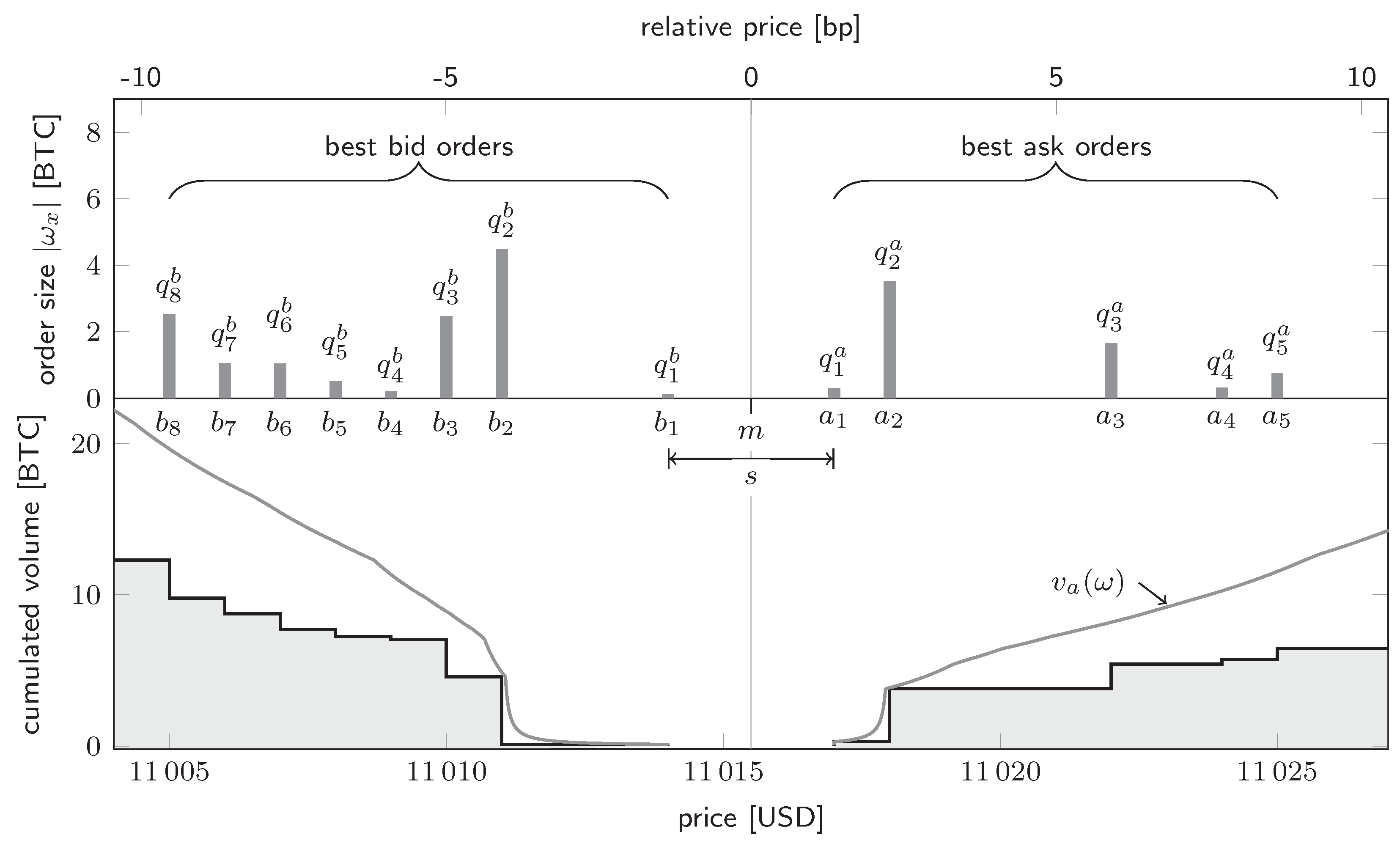
We first focus on derived measures of the static LOB at some time t, i.e., $\mathcal{L}\left(t\right)$. In other words, we consider some function f which we apply to the static state of the LOB, i.e., $f\left(\mathcal{L}\right(t\left)\right)$. Most of the quantities introduced in this section are visualized in Figure 1. One of the most important properties of $\mathcal{L}\left(t\right)$ is its depth profile, which is the total available limit order volume at a given price p and is given by

$$n^b(p,t)=\sum _{\{x\in \mathcal{B}\left(t\right)|p_x=p\}}{\omega }_x,$$

(1)

for the bid side, and similarly for the ask side. We write the i-th best price of the ask side (bid side) as $a_i\left(t\right),i\in \{1,\cdots ,|\mathcal{A}\left(t\right)\left|\right\}$ ($b_i\left(t\right),i\in \{1,\cdots ,|\mathcal{B}\left(t\right)\left|\right\}$). The total order volume at level i is given by $q_i^a\left(t\right)=n^a(a_i\left(t\right),t)$ and $q_i^b\left(t\right)=n^b(b_i\left(t\right),t)$, respectively. The first ask-side level $a_1\left(t\right)={min}_{x\in \mathcal{A}\left(t\right)}{p}_x$ is the best ask price of the order book, and $b_1\left(t\right)={max}_{x\in \mathcal{B}\left(t\right)}{p}_x$ is the best bid price. The average of best ask and best bid price is the mid price given by $m\left(t\right)=\left(a_1\left(t\right)+b_1\left(t\right)\right)/2$. The difference between the best ask and the best bid price is the bid-ask spread, i.e., $s\left(t\right)=a_1\left(t\right)-b_1\left(t\right)$. Similarly, we can define the volume-weighted average price (VWAP) function for the imaginary immediate execution of a market order of size $\omega$, assuming no other orders interfere at the same instant:

$$v_a(\omega ,t)=\frac{1}{\omega }\sum _i{a}_i\left(t\right)·min\left(max\left(\omega -\sum _{k=1}^i{q}_k^a\left(t\right),0\right),q_i^a\left(t\right)\right).$$

(2)

Herein, the index i iterates over price levels in a price-ordered fashion, and we assume that the order book is deep enough to provide the requested volume $\omega$. The definition for the bid-side VWAP function $v_b(\omega ,t)$ is analogous.

To increase the comparability of different order books at different times, it is common practice to consider prices relative to the current mid price. We define the transformation of a price $p\left(t\right)$ to the relative price scale as $\tilde{p}\left(t\right)=(p\left(t\right)-m\left(t\right))/m\left(t\right)$. In this scale, the relative bid-ask spread is given by $\tilde{s}\left(t\right)=\tilde{a}\left(t\right)-\tilde{b}\left(t\right)$. The bid-ask spread often serves as a measure of market liquidity, as it quantifies the liquidity premium one needs to pay for immediately executing a trade by submitting a market order. However, it is only an accurate estimate for the liquidity premium for order volumes smaller than the order book depth at the best bid/best ask price. To correctly valuate the liquidity cost for a given volume $\omega$, we can similarly define the two-sided VWAP spread as $\widetilde{vs}(\omega ,t)={\tilde{v}}_a(\omega ,t)-{\tilde{v}}_b(\omega ,t)$.2

We split further analyses on measures of the static LOB into three canonical subgroups: First, we can perform cross-sectional descriptive statistics in the sense that we ignore the time series nature of the data. Second, we can take the time series nature of the derived measures into account and study their evolution over time. Third, we can evaluate descriptive statistics of derived measures subject to some condition.3

Table 2. Overview of commonly found facts and supporting analyses on static limit order books. Type refers to the class of analysis and is one of U (unconditional statistic), TS (time series statistic) and C (conditional  statistic).

Common Fact	Measure Considered for Analysis	Key References	Type
Symmetric mean cumulative depth profiles	Time-averaged depth profile ${(\overline{\tilde{a}},\overline{\tilde{b}},\overline{q^a},\overline{q^b})}_i$ (Equations (3) and (4)) and time-averaged relative price differences between adjacent steps of the LOB ${(\overline{\Delta \tilde{a}},\overline{\Delta \tilde{b}})}_i$ (Equation (5))	Biais et al. (1995), Cao et al. (2009) and Potters and Bouchaud (2003)	U
Gamma-distributed depth at best bid and best ask	Unconditional empirical distribution of the total volume (depth) at the best bid (or ask), i.e., ${\left\{q_0^a\left(t\right)\right\}}_t$ and $\{{\left(q_0^b\left(t\right)\right\}}_t$	Bouchaud et al. (2002)	U
Hump-shaped mean depth profile	Empirical distribution of the time-averaged volume from the depth profile ($q_i^a\left(t\right)$ and $q_i^b\left(t\right)$) as a function of the (relative) price difference to the ask or bid price	Bouchaud et al. (2002), Potters and Bouchaud (2003) and Gu et al. (2008)	U
Increase in liquidity costs beyond the best bid/ask	Unconditional distribution of the relative bid-ask spread ${\left\{\tilde{s}\left(t\right)\right\}}_t$ and the relative VWAP spread ${\left\{\widetilde{vs}(\omega ,t)\right\}}_t$	Gomber et al. (2015)	U
Heavy tails of mid-price returns	Unconditional distribution of mid-price returns ${\left\{r(t,\Delta t)\right\}}_t$ analyzed with kurtosis estimates and Hill estimator (Equations (10) and (11))	Hill (1975), Balanda and MacGillivray (1990) and Lux and Marchesi (2000)	TS
No autocorrelation of returns	Autocorrelation of logarithmic mid-price returns $C\left(n\right)$ (Equation (8))	Lux and Marchesi (2000) and Cont (2001)	TS
Volatility clustering	Autocorrelation of absolute or squared logarithmic mid-price returns, i.e., the functions $C_1\left(n\right)$ and $C_2\left(n\right)$, respectively (Equation (9))	Lux and Marchesi (2000) and Cont (2001)	TS
Non-constant liquidity costs	Average daily liquidity costs (i.e., the bid-ask spread $\tilde{s}\left(t\right)$ and the VWAP spread $\widetilde{vs}(\omega ,t)$)	Dyhrberg et al. (2018)	TS
U-shaped intraday patterns of liquidity costs	Average liquidity costs (i.e., the bid-ask spread $\tilde{s}\left(t\right)$ and the VWAP spread $\widetilde{vs}(\omega ,t)$) conditional on the hour of the day	McInish and Wood (1992) and Gomber et al. (2015)	C
Liquidity resiliency and timed large trades	Distribution of average liquidity costs (i.e., the bid-ask spread $\tilde{s}\left(t\right)$ and the VWAP spread $\widetilde{vs}(\omega ,t)$) for large trades conditional on the event time $\tau$ of the trade (Equation (12))	Cummings and Frino (2010) and Gomber et al. (2015)	C

provides an overview of the analyses which we describe in the following, and includes the commonly observed fact under investigation as well as relevant references from works focusing on traditional limit order markets.

4.2.1. Descriptive Statistics of Unconditional Limit Order Book Measures

We can now introduce cross-sectional statistics of measures based on the static LOB $\mathcal{L}\left(t\right)$. We start from a set of T LOB states ${\left\{\mathcal{L}\left(t\right)\right\}}_{t=1}^T$ and derive the corresponding set of values of some measure f, i.e., ${\left\{f\left(\mathcal{L}\left(t\right)\right)\right\}}_{t=1}^T$. In a first set of analyses, we consider distributional characteristics of the values of f. Thereby, we focus on two important measures for liquidity costs, namely on the relative bid-ask spread ($f=\tilde{s}$) and on the two-sided VWAP spread for different order volumes $\omega$ ($f=\widetilde{vs}$). The second set of analyses considers the average depth profile, where we average over all states $\mathcal{L}\left(t\right)$ of the LOB at different points in time t. We first define the time-averaged relative ask (bid) price of LOB step i, i.e.,

$$\overline{{\tilde{a}}_i}=\frac{1}{T}\sum _{t=1}^T{\tilde{a}}_i\left(t\right)\mathrm{and}\overline{{\tilde{b}}_i}=\frac{1}{T}\sum _{t=1}^T{\tilde{b}}_i\left(t\right).$$

(3)

Following Biais et al. (1995), we consider the time-averaged cumulated depth up to a step i, i.e.,

$$\overline{q_i^a}=\frac{1}{T}\sum _{t=1}^T\sum _{j=1}^i{q}_j^a\left(t\right)\mathrm{and}\overline{q_i^b}=\frac{1}{T}\sum _{t=1}^T\sum _{j=1}^i{q}_j^b\left(t\right).$$

(4)

The vectors ${\left(\overline{\tilde{a}},\overline{\tilde{b}},\overline{q^a},\overline{q^b}\right)}_i$ represent the time-averaged shape of the cumulated LOB. A different definition is used by Bouchaud et al. (2002) to discuss the average shape of the LOB: They consider the time-averaged distribution of non-cumulated volume $q_i^a$ (or $q_i^b$) as a function of the difference in price to the current bid or ask. Complementing the analyses of the average shape of the order book, we also consider time-averaged differences between the relative price at level i and level $i+1$, i.e.,

$$\overline{\Delta {\tilde{a}}_i}=\frac{1}{T}\sum _{t=1}^T{\tilde{a}}_{i+1}\left(t\right)-{\tilde{a}}_i\left(t\right)\mathrm{and}\overline{\Delta {\tilde{b}}_i}=\frac{1}{T}\sum _{t=1}^T{\tilde{b}}_{i+1}\left(t\right)-{\tilde{b}}_i\left(t\right).$$

(5)

4.2.2. Time Series Properties of Limit Order Book Measures

Instead of considering cross-sectional properties of the LOB state $\mathcal{L}\left(t\right)$, we can consider the time series of values of some measure f, i.e., ${\left(f\left(\mathcal{L}\left(t\right)\right)\right)}_{t=1}^T$. Our analyses will focus on measures of liquidity costs (relative bid-ask spread $\tilde{s}$ and the two-sided VWAP spread $f=\widetilde{vs}$) and the mid price m. Also, we consider logarithmic mid-price returns on the time scale $\Delta t$ given by

$$r^{mid}(t,\Delta t)=ln\left(m(t+\Delta t)\right)-ln\left(m\left(t\right)\right).$$

(6)

We calculate the log-realized volatility $rv(t_1,t_2,\Delta t)$ between times $t_1$ and $t_2$ as

$$rv(t_1,t_2,\Delta t)=\sqrt{\sum _{t=t_1}^{t_2}{\left(r^{mid}(t,\Delta t)\right)}^2}.$$

(7)

Following Cont (2001), we also compute the autocorrelation function of logarithmic mid-price returns and the k-th power of absolute logarithmic mid-price returns, i.e.,

$$\begin{array}{ccc}\hfill C^{mid}\left(n\right)& =& \mathrm{corr}\left(r^{mid}(t,\Delta t),r^{mid}(t+n\Delta t,\Delta t)\right),\mathrm{and}\hfill \end{array}$$

(8)

$$\begin{array}{ccc}\hfill C_k^{mid}\left(n\right)& =& \mathrm{corr}\left({\left|r^{mid}(t,\Delta t)\right|}^k,{\left|r^{mid}(t+n\Delta t,\Delta t)\right|}^k\right).\hfill \end{array}$$

(9)

Herein, n denotes the lag, and corr is the sample correlation function.

Tails of the distribution of mid-price returns are analyzed in terms of two kurtosis measures and a tail index estimator. As kurtosis metrics we consider the empirical fourth standardized moment (henceforth: m${}_4$, compare Bacon (2008)) and a second metric based on Balanda and MacGillivray (1990), using quantiles (henceforth: ${\gamma }_{p,q}$). The computation of ${\gamma }_{p,q}$ is as follows:

$$\begin{array}{c}\hfill {\gamma }_{p,q}=\frac{F^{-1}\left(1-p\right)-F^{-1}\left(p\right)}{F^{-1}\left(1-q\right)-F^{-1}\left(q\right)},\mathrm{with}0<p<q<0.5.\end{array}$$

(10)

Please note that $F^{-1}$ denotes the quantile function and p and q are p-quantiles. If the underlying distribution F is symmetric, then we can use ${\gamma }_{p=0.025,q=0.125}$ to measure heavy tails (Büning 1991). To measure deviation from normality we compute the excess version of both metrics, i.e., ${\gamma }_{p=0.025,q=0.125}^e={\gamma }_{p=0.025,q=0.125}-1.706$ and $m_4^e=m_4-3$. A time series is classified as platykurtic if the excess metric of interest is smaller than zero, mesokurtic if the excess metric is equal to zero and leptokurtic if the excess metric is larger than zero. Thereby, for both metrics larger positive values are associated with heavier tails, while smaller negative values indicate lighter tails. Financial time series are typically leptokurtic (Cont 2001).

The tail index is a measure of the frequency of extreme returns (Lux and Marchesi 2000) and is estimated with a Hill estimator (Hill 1975). As a prerequisite to compute the Hill estimator the time series must be descendingly ordered, i.e., $r_n^{mid}\ge \cdots \ge r_{n-a}^{mid}\ge \cdots \ge r_1^{mid}$. Thereby, $r_n^{mid}$ denotes the largest mid-price return in the time series and $r_1^{mid}$ the smallest. The number of observations included in the tail analysis solely depends on the value for a. In recent decades a large body of literature has focused on how to determine a.4 Following Lux and Marchesi (2000) and Kelly and Jiang (2014), we set a to a fixed percentage p of data points, namely 10, 5 and $2.5$ percent. Given the ordered time series, we can compute the Hill estimator with the following equation (Lux and Marchesi 2000):

$$\begin{array}{c}\hfill H_p=\frac{1}{\frac{1}{a}\sum _{l=1}^a\left[ln\left(r_{n-l+1}^{mid}\right)-ln\left(r_{n-a}^{mid}\right)\right]}.\end{array}$$

(11)

4.2.3. Statistics of Conditional Limit Order Book Measures

In the third category, we subsume many analyses from the literature which evaluate measures of the static LOB conditional on some condition $\mathcal{C}$. Following our notation, we evaluate order book measures f for the subset given by $\mathcal{C}$, i.e., consider the set $\left\{f\right(\mathcal{L}\left(t\right)\left)\right|\mathcal{L}\left(t\right)\in \mathcal{C}\}$. We investigate the intraday dynamics of liquidity measures to test for commonly observed patterns—see, among others, McInish and Wood (1992), Biais et al. (1995), Danielsson and Payne (2001), Ranaldo (2004) and Gomber et al. (2015). In this case, $\mathcal{C}$ selects only those order book states from a given hour of the day, and we evaluate mean bid-ask spreads ($f=\tilde{s}$) and VWAP spreads ($f=\widetilde{vs}$). Another class of studies covers the concept of market resiliency, which we define in the sense of Foucault et al. (2005) and Gomber et al. (2015) as the recovery of market liquidity following liquidity shocks, and which is considered to be one of the main characteristics of liquid markets (Black 1971; Kyle 1985). We follow several previous studies (compare, for example, Degryse et al. (2005), Large (2007), Cummings and Frino (2010) and Gomber et al. (2015)) and analyze the evolution of market liquidity around large trades in a conditional event study: We condition the analysis onto a set of selected events ${\mathcal{E}}_{\mathcal{C}}$, which is given by the set of trades with exceptionally large volume, and transform the timestamp t of a LOB state $\mathcal{L}\left(t\right)$ to the event time scale $\tau$ of event e, i.e., calculate $\tau =t-t_e$. We then consider the average avg of a measure f over all LOB states that are a time difference $\tau$ away from a selected trade $e\in {\mathcal{E}}_{\mathcal{C}}$:

$$\overline{f}\left(\tau \right)=\mathrm{avg}\left(\left\{f\left(\mathcal{L}\left(t\right)\right)|t-t_e=\tau ,e\in {\mathcal{E}}_{\mathcal{C}}\right\}\right).$$

(12)

In the analyses presented in this paper, $\overline{f}$ evaluates averages of the bid-ask spread and the VWAP spread around large trades.

4.3. Dynamics of the Limit Order Book: Order and Trade Flows

We now turn to the analysis of the two event streams translating one static state of the LOB $\mathcal{L}\left(t_1\right)$ to a subsequent state $\mathcal{L}\left(t_2\right)$: the flow of limit orders $\left\{x_i\right\}$ leading to changes of the order book and the resulting flow of trades $\left\{M_i\right\}$. We use the index i to count limit order or trade events, while index t refers to the wall-clock time. We directly observe trades with information $M_i={(p_M,{\omega }_M,t_M)}_i$, with the traded amount $|{\omega }_M|$, the execution price $p_M$ and its time $t_M$. The sign of ${\omega }_M$ is determined by the order initiating the trade. In contrast, we are unable to observe every single limit order between LOB states at different times. Nevertheless, we can compute the change in depth profile between order book states sampled at times t and $t+\Delta t$ as the absolute change in limit order depth at a given price p, i.e.,

$$\Delta n^b(p,t)=|n^b(p,t+\Delta t)-n^b(p,t)|$$

(13)

for the bid side, and similarly for the ask side. For newly submitted or canceled limit orders that are not executed, $\Delta n^b(p,t)$ corresponds to the net limit order volume flow between t and $t+\Delta t$. The limit order volume flow close to the current price is underestimated as some orders are executed in between.

As for static LOB measures, we use three canonical subgroups (unconditional, time series and conditional properties) to structure our analyses.

Table 3. Overview of commonly found facts and supporting analyses on trades and limit orders. Type refers to the class of analysis and is one of U (unconditional statistic), TS (time series statistic) and C (conditional statistic).

Common Fact	Measure Considered for Analysis	Key References	Type
Number preference for trade sizes	Empirical distribution of trade size ${\omega }_M$	Mu et al. (2009)	U
Power tail in the distribution of trade size	Empirical distribution of trade size ${\omega }_M$	Gopikrishnan et al. (2000), Maslov and Mills (2001) and Mu et al. (2009)	U
Power-law decay of order frequency with relative price	Time-average of changed limit order volume, i.e., $\overline{\Delta n^b\left(p\right)}$ and $\overline{\Delta n^a\left(p\right)}$ (Equation (14))	similar to Bouchaud et al. (2002) and Zovko and Farmer (2002)	U
Negative autocorrelation of trade prices (bid-ask bounce)	Autocorrelation of the series of trade price changes $C^{tp}\left(n\right)$ (Equation (15))	Cont (2001) and Russell and Engle (2010)	TS
Autocorrelation of trade sizes	Autocorrelation in the series of trade sizes $C^{size}\left(n\right)$ (Equation (16))		TS
Intraday patterns in trade frequency and volume	Average trade frequency and average trade size conditional on the hour of the day	Biais et al. (1995) and Danielsson and Payne (2001)	C

provides an analogous overview of analyses with commonly found facts from other works.

4.3.1. Descriptive Statistics of Unconditional Measures

Several authors study the frequency of limit orders and their size as a function of the price difference to the current bid or ask (among others, Bouchaud et al. (2002), Potters and Bouchaud (2003) and Gu et al. (2008)). To analyze the limit order flow as a function of price using available data, we consider the time-averaged absolute change in limit order depth as a function of price, which is for the bid side given by

$$\overline{\Delta n^b\left(p\right)}=\frac{1}{T}\sum _{t=1}^T\Delta n^b(p,t),$$

(14)

and analogously for the ask side ($\overline{\Delta n^a\left(p\right)}$). Another class of works studies the empirical frequency distribution of transaction sizes, for example Gopikrishnan et al. (2000), Maslov and Mills (2001) and Mu et al. (2009). We repeat these analyses with the available cryptocurrency data and consider distributional properties of the series of trade size, i.e., $\left\{{\omega }_{M_i}\right\}$.

4.3.2. Time Series Properties

To evaluate the evolution of trade properties, we sample trade data onto lower timescales by considering some trade statistics $f_T$ of all transactions between time $t_1$ and $t_2$, i.e., the set $\left\{M_i\right|t_1\le t_{M_i}<t_2\}$. We consider the average trade size, the total trade volume as well as trade counts (i.e., the trade frequency).

Time series of changes in trade price are known to exhibit autocorrelation for the first few lags (compare, for example, Cont (2001) and Russell and Engle (2010)). We therefore define the series of changes between trade prices, i.e., $\Delta p_i=p_{M_{i+1}}-p_{M_i}$, and compute its autocorrelation as

$$C^{tp}\left(n\right)=\mathrm{corr}\left(\Delta p_i,\Delta p_{i+n}\right).$$

(15)

Similarly, we analyze the autocorrelation in the series of trade sizes by considering

$$C^{size}\left(n\right)=\mathrm{corr}\left({\omega }_{M_i},{\omega }_{M_{i+n}}\right).$$

(16)

4.3.3. Statistics of Conditional Trade Measures

Similar to the analysis of intraday patterns of liquidity costs, we consider average properties of cryptocurrency transactions conditional on the hour of the day (trade frequency, total traded volume, average trade size). Biais et al. (1995) and Danielsson and Payne (2001) perform similar analyses.

5. Results

Following the methodology outlined in the previous section, we now present results for the cryptocurrency exchange BitFinex and the currency pair BTC/USD. We focus our analyses on this exchange as it has the highest trading volume in the time period of our study. We also evaluate data for the currency pair BTC/USD for the second and third largest exchange (Coinbase and Bitstamp), and compare the results to check robustness. Parts of those results are included in the appendix, and we discuss major differences in the following. Most LOB measures are unlikely to be stationary, and might therefore differ with market phases. To check robustness in this regard, we divide our data into a subperiod of high volatility (SP1 from 2 December 2017 to 7 May 2018) and a subperiod with relatively stable prices (SP2 from 7 May 2018 to 12 October 2018).5 We first analyze statistics of measures of the static LOB in Section 5.1, which we divide into three parts to separately discuss unconditional, time series and conditional statistics. In Section 5.2, we analyze the dynamics of LOBs.

5.1. Analysis of the Static Limit Order Book

5.1.1. Descriptive Statistics of Unconditional Limit Order Book Measures

We first present unconditional descriptive statistics of measures of the static LOB, and begin by discussing the average shape of the LOB.

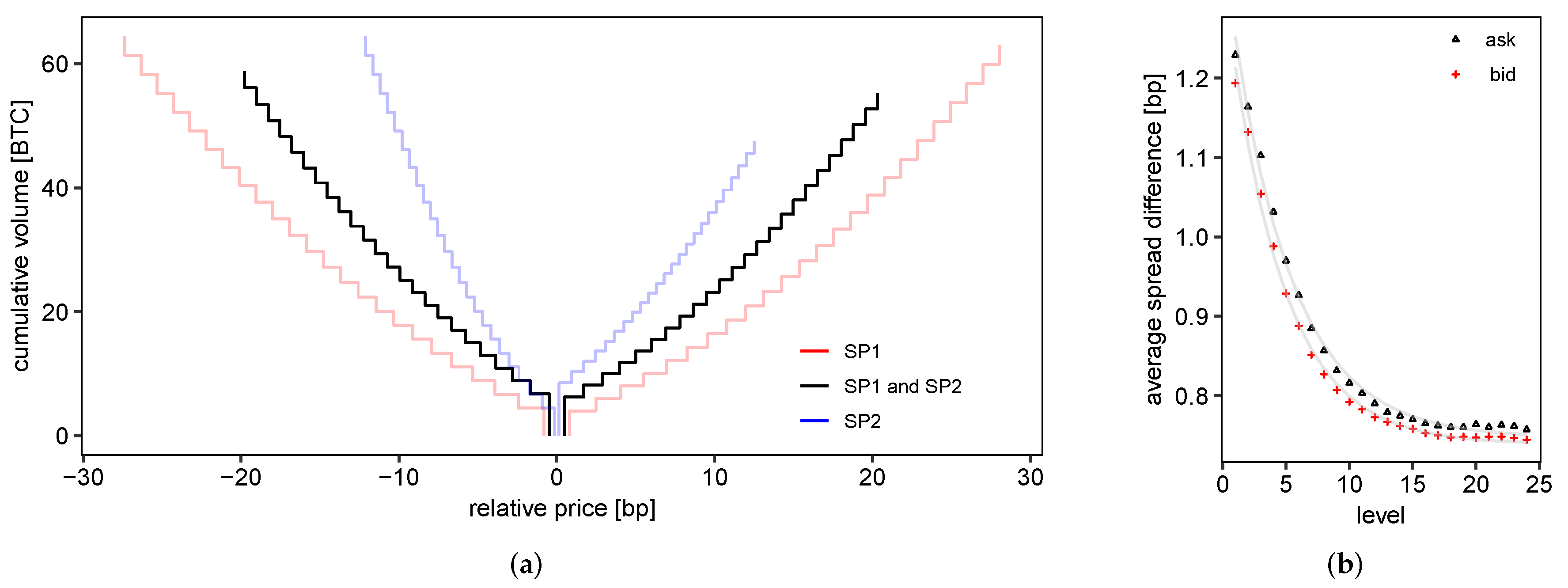
Time-averaged depth profile:Figure 2a displays the time-averaged cumulated depth profile of the LOB, i.e., plots the quantities ${(\overline{\tilde{a}},\overline{\tilde{b}},\overline{q^a},\overline{q^b})}_i$ (Equations (3) and (4)) for the first 25 limit orders of each side, on a relative price scale.

Table 4. Descriptive statistics of the average order book. The table reports descriptive statistics for the relative prices (${\tilde{a}}_i$ and ${\tilde{b}}_i$) and depths ($q_i^a$ and $q_i^b$) at the first ten steps of the LOB.

	${\tilde{\mathit{a}}}_1$ [bp]	${\tilde{\mathit{a}}}_2$ [bp]	${\tilde{\mathit{a}}}_3$ [bp]	${\tilde{\mathit{a}}}_4$ [bp]	${\tilde{\mathit{a}}}_5$ [bp]	${\tilde{\mathit{a}}}_6$ [bp]	${\tilde{\mathit{a}}}_7$ [bp]	${\tilde{\mathit{a}}}_8$ [bp]	${\tilde{\mathit{a}}}_9$ [bp]	${\tilde{\mathit{a}}}_{10}$ [bp]
mean	0.4831	1.7123	2.8763	3.9788	5.0104	5.9803	6.9070	7.7917	8.6484	9.4799
sd	1.2024	2.3147	2.9969	3.6133	4.1442	4.6576	5.1445	5.6122	6.0846	6.5424
q25	0.0675	0.3759	1.0092	1.6425	2.3193	2.9572	3.5081	4.0941	4.6438	5.1234
median	0.0777	1.0470	2.0961	3.0733	3.9880	4.8294	5.5362	6.2500	6.9267	7.5638
q75	0.4392	2.1786	3.7341	5.1103	6.4375	7.6628	8.8376	9.9623	11.0422	12.1047
	${\tilde{\mathit{b}}}_{\mathbf{1}}$[bp]	${\tilde{\mathit{b}}}_{\mathbf{2}}$[bp]	${\tilde{\mathit{b}}}_{\mathbf{3}}$[bp]	${\tilde{\mathit{b}}}_{\mathbf{4}}$[bp]	${\tilde{\mathit{b}}}_{\mathbf{5}}$[bp]	${\tilde{\mathit{b}}}_{\mathbf{6}}$[bp]	${\tilde{\mathit{b}}}_{\mathbf{7}}$[bp]	${\tilde{\mathit{b}}}_{\mathbf{8}}$[bp]	${\tilde{\mathit{b}}}_{\mathbf{9}}$[bp]	${\tilde{\mathit{b}}}_{\mathbf{10}}$[bp]
mean	−0.4831	−1.6766	−2.8087	−3.8629	−4.8509	−5.7797	−6.6675	−7.5188	−8.3457	−9.1531
sd	1.2024	2.2548	2.9204	3.4579	3.9502	4.4140	4.8690	5.3263	5.7785	6.2391
q25	−0.4392	−2.1422	−3.6505	−5.0113	−6.2035	−7.3812	−8.4742	−9.5624	−10.6170	−11.6707
median	−0.0777	−1.0301	−2.0679	−3.0492	−3.9324	−4.7487	−5.3844	−6.0720	−6.7132	−7.3242
q75	−0.0675	−0.3608	−0.9902	−1.6176	−2.2711	−2.9088	−3.4496	−4.0167	−4.5456	−5.0245
	${\mathit{q}}_{\mathbf{1}}^{\mathit{a}}$[BTC]	${\mathit{q}}_{\mathbf{2}}^{\mathit{a}}$[BTC]	${\mathit{q}}_{\mathbf{3}}^{\mathit{a}}$[BTC]	${\mathit{q}}_{\mathbf{4}}^{\mathit{a}}$[BTC]	${\mathit{q}}_{\mathbf{5}}^{\mathit{a}}$[BTC]	${\mathit{q}}_{\mathbf{6}}^{\mathit{a}}$[BTC]	${\mathit{q}}_{\mathbf{7}}^{\mathit{a}}$[BTC]	${\mathit{q}}_{\mathbf{8}}^{\mathit{a}}$[BTC]	${\mathit{q}}_{\mathbf{9}}^{\mathit{a}}$[BTC]	${\mathit{q}}_{\mathbf{10}}^{\mathit{a}}$[BTC]
mean	6.2519	1.9335	1.8313	1.8295	1.8376	1.8579	1.8727	1.8916	1.8991	1.9668
sd	20.2119	14.0038	9.5268	9.3860	10.6332	9.5688	9.6347	10.2464	9.9094	17.8200
q25	0.5049	0.1000	0.1000	0.1049	0.1093	0.1226	0.1270	0.1322	0.1300	0.1338
median	2.1400	0.5225	0.5008	0.5000	0.5000	0.5000	0.5000	0.5000	0.5000	0.5000
q75	6.6157	1.6600	1.5000	1.4802	1.4634	1.4722	1.4860	1.4990	1.5000	1.5000
	${\mathit{q}}_{\mathbf{1}}^{\mathit{b}}$[BTC]	${\mathit{q}}_{\mathbf{2}}^{\mathit{b}}$[BTC]	${\mathit{q}}_{\mathbf{3}}^{\mathit{b}}$[BTC]	${\mathit{q}}_{\mathbf{4}}^{\mathit{b}}$[BTC]	${\mathit{q}}_{\mathbf{5}}^{\mathit{b}}$[BTC]	${\mathit{q}}_{\mathbf{6}}^{\mathit{b}}$[BTC]	${\mathit{q}}_{\mathbf{7}}^{\mathit{b}}$[BTC]	${\mathit{q}}_{\mathbf{8}}^{\mathit{b}}$[BTC]	${\mathit{q}}_{\mathbf{9}}^{\mathit{b}}$[BTC]	${\mathit{q}}_{\mathbf{10}}^{\mathit{b}}$[BTC]
mean	6.7553	2.1255	2.0309	2.0423	2.0494	2.0255	1.9986	2.0195	2.0211	2.0247
sd	21.0636	10.3102	11.5825	12.0838	11.7907	12.6380	12.7130	12.8436	12.1750	10.6579
q25	0.5972	0.1000	0.1000	0.1000	0.1000	0.1063	0.1121	0.1194	0.1270	0.1251
median	2.2928	0.5394	0.5000	0.5000	0.5000	0.5000	0.5000	0.5000	0.5000	0.5000
q75	6.8141	1.7280	1.5360	1.5000	1.4770	1.4512	1.4300	1.4440	1.4743	1.5000

presents further descriptive statistics of the prices and volumes of the first ten steps of the depth profile. We make the following observations:

• Symmetry between bid and ask side: There is a high degree of symmetry in the average depth profile of the bid and the ask side: Average prices exhibit very similar absolute values, and depths agree surprisingly well at corresponding steps i. This symmetry is well-known for limit order stock markets (see, for example, Biais et al. (1995), Potters and Bouchaud (2003) and Cao et al. (2009)).
• Dispersion of liquidity: The liquidity provided at the best bid or the best ask price is only a very small part of overall liquidity, and the incremental liquidity provided by each level deeper in the LOB is comparably small. Biais et al. (1995) observe this pattern for equity data from the Paris Bourse, and we find that it is very pronounced in the Bitcoin market: The average level contributes an additional volume of $2\mathrm{BTC}$ (corresponding to roughly 20000 USD). These small depths may be driven by the fact that the cryptocurrency markets are still dominated by retail trading activity, and that there is still potential for further institutional market making activities—see Chaparro (2017) and Arnold (2018). Furthermore, we find that the average volume at the best ask/bid is triple the volume contributed by levels deeper in the book, which contrasts with Biais et al. (1995) who point out that it is slightly lower.
• Approximately linear price schedule: In agreement with Biais et al. (1995), we observe that the price schedule, i.e., the dependence of the price on demanded or offered quantity, can be approximated very well by linearity and is weakly concave. The concavity seems to be a consequence of an unequal spacing of average price levels rather than a consequence of increasing average volume at each price level. To analyze this in detail, Figure 2b displays the average relative spread between adjacent price levels ${\left(\overline{\Delta \tilde{a}},\overline{\Delta \tilde{b}}\right)}_i$ (Equation (5)) as function of the level number i. The bid and the ask side of the LOB behave very similarly. The largest average difference in price is found directly after the best bid/best ask and amounts to roughly 1.2 bp, which is larger than the average bid-ask spread (0.97 bp). This value then declines to lower values and remains constant at roughly 0.7 bp for higher price levels ($i\ge 15$).6 The first 25 price levels in the static LOB are therefore denser further away from the bid-ask spread. We might interpret this observation as a consequence of the execution of market orders reducing the limit order volume at the center of the LOB. Orders deeper in the book are less likely to be executed, leading to more densely spaced price levels on average.

Robustness checks: The observed symmetry between bid and ask side of the LOB and the roughly linear price schedule holds also for subperiods SP1 and SP2 (compare the light gray lines in Figure 2a) as well as for the Coinbase and Bitstamp exchanges (compare Figure A1 in the Appendix A). Surprisingly, for Coinbase, the price schedule is convex, and consequently, the average price spread between LOB levels increases with i.

Distribution of volume at the (best) bid and ask:Figure 3 shows the joint distribution of volume at the best bid and the best ask ($q_1^b$ and $q_1^a$, respectively). We calculate the common logarithm of the volume in units of the minimum order size (0.002 BTC, compare Table 1) and calculate the histogram. The empirical distribution shares the main characteristic properties with the results by Bouchaud et al. (2002) for the Paris Bourse: First, the empirical distributions agree very well and fit to a Gamma distribution $p\left(q_1\right)\propto q_1^{\gamma -1}exp\left(-q_1/\theta \right)$ with a shape parameter $\gamma \approx 0.28\le 1$ and a scale parameter $\theta \approx 10.94\mathrm{BTC}$. From the fit to the Gamma distribution follows that the most probable volume at the best bid or best ask is zero, but the expected value is rather large. Second, the distribution deviates from the Gamma distribution for specific, equally spaced values: Apparently, there is a number preference for the order size, which gets apparent for smaller depth values, where it is more likely that only a single limit order provides the complete depth. Preferred values seem to be 0.1 BTC, 0.5 BTC, and especially 1.0 BTC. Third, the distributions of the bid and the ask side are very similar (not shown).

Robustness checks: Despite differences in estimated parameters $\gamma$ and $\theta$, we find the empirical distribution for subperiods SP1 and SP2 to be very similar. When comparing results to those of the Coinbase and Bitstamp exchanges, we find that the volume at the best bid and best ask is considerably lower (compare

Table A1. Descriptive statistics of the average order book for the Coinbase BTC/USD market. The  table reports descriptive statistics for the relative prices (${\tilde{a}}_i$ and ${\tilde{b}}_i$) and depths ($q_i^a$ and $q_i^b$) at the first five limit order steps.

	${\tilde{\mathit{a}}}_1$ [bp]	${\tilde{\mathit{a}}}_2$ [bp]	${\tilde{\mathit{a}}}_3$ [bp]	${\tilde{\mathit{a}}}_4$ [bp]	${\tilde{\mathit{a}}}_5$ [bp]	${\tilde{\mathit{b}}}_1$ [bp]	${\tilde{\mathit{b}}}_2$ [bp]	${\tilde{\mathit{b}}}_3$ [bp]	${\tilde{\mathit{b}}}_4$ [bp]	${\tilde{\mathit{b}}}_5$ [bp]
mean	0.0992	0.1532	0.3097	0.5102	0.7390	−0.0992	−0.1638	−0.3407	−0.5685	−0.8364
sd	9.4231	0.9120	1.3032	1.6700	2.0189	9.4231	0.9466	1.3670	1.7763	2.2484
q25	0.0056	0.0057	0.0058	0.0060	0.0061	−0.0076	−0.0077	−0.0078	−0.0085	−0.4824
median	0.0067	0.0068	0.0071	0.0074	0.0075	−0.0067	−0.0068	−0.0070	−0.0073	−0.0075
q75	0.0076	0.0077	0.0078	0.0085	0.3317	−0.0056	−0.0057	−0.0058	−0.0059	−0.0060
	${\mathit{q}}_{\mathbf{1}}^{\mathit{a}}$[BTC]	${\mathit{q}}_{\mathbf{2}}^{\mathit{a}}$[BTC]	${\mathit{q}}_{\mathbf{3}}^{\mathit{a}}$[BTC]	${\mathit{q}}_{\mathbf{4}}^{\mathit{a}}$[BTC]	${\mathit{q}}_{\mathbf{5}}^{\mathit{a}}$[BTC]	${\mathit{q}}_{\mathbf{1}}^{\mathit{b}}$[BTC]	${\mathit{q}}_{\mathbf{2}}^{\mathit{b}}$[BTC]	${\mathit{q}}_{\mathbf{3}}^{\mathit{b}}$[BTC]	${\mathit{q}}_{\mathbf{4}}^{\mathit{b}}$[BTC]	${\mathit{q}}_{\mathbf{5}}^{\mathit{b}}$[BTC]
mean	1.0937	1.0352	1.0407	1.0242	1.0012	0.8994	0.8716	0.8330	0.8478	0.8355
sd	3.5183	3.4218	3.5283	3.5174	3.5246	2.7554	2.7223	2.6287	2.7821	2.7304
q25	0.0047	0.0029	0.0030	0.0025	0.0023	0.0077	0.0064	0.0060	0.0063	0.0063
median	0.1130	0.1000	0.0932	0.0800	0.0662	0.1200	0.1002	0.1000	0.1000	0.0958
q75	1.0000	1.0000	1.0000	1.0000	1.0000	1.0000	1.0000	0.9725	0.9683	0.9460

and

Table A2. Descriptive statistics of the average order book for the Bitstamp BTC/USD market. The table reports descriptive statistics for the relative prices (${\tilde{a}}_i$ and ${\tilde{b}}_i$) and depths ($q_i^a$ and $q_i^b$) at the first five limit order steps.

	${\tilde{\mathit{a}}}_1$ [bp]	${\tilde{\mathit{a}}}_2$ [bp]	${\tilde{\mathit{a}}}_3$ [bp]	${\tilde{\mathit{a}}}_4$ [bp]	${\tilde{\mathit{a}}}_5$ [bp]	${\tilde{\mathit{b}}}_1$ [bp]	${\tilde{\mathit{b}}}_2$ [bp]	${\tilde{\mathit{b}}}_3$ [bp]	${\tilde{\mathit{b}}}_4$ [bp]	${\tilde{\mathit{b}}}_5$ [bp]
mean	3.9306	5.9740	7.8983	9.6986	11.3785	−3.9306	−6.2516	−8.3233	−10.2498	−12.0205
sd	3.6971	5.0798	5.9524	6.6103	7.1657	3.6971	5.2242	6.1008	6.7221	7.2437
q25	1.3370	2.6456	3.9142	5.1897	6.5248	−5.3879	−7.9980	−10.6020	−12.8396	−14.7508
median	3.1511	4.7447	6.4603	8.2124	9.8818	−3.1511	−4.9946	−6.9114	−8.8283	−10.5893
q75	5.3879	7.6499	10.1350	12.3066	14.2027	−1.3370	−2.8920	−4.3039	−5.7707	−7.2550
	${\mathit{q}}_{\mathbf{1}}^{\mathit{a}}$[BTC]	${\mathit{q}}_{\mathbf{2}}^{\mathit{a}}$[BTC]	${\mathit{q}}_{\mathbf{3}}^{\mathit{a}}$[BTC]	${\mathit{q}}_{\mathbf{4}}^{\mathit{a}}$[BTC]	${\mathit{q}}_{\mathbf{5}}^{\mathit{a}}$[BTC]	${\mathit{q}}_{\mathbf{1}}^{\mathit{b}}$[BTC]	${\mathit{q}}_{\mathbf{2}}^{\mathit{b}}$[BTC]	${\mathit{q}}_{\mathbf{3}}^{\mathit{b}}$[BTC]	${\mathit{q}}_{\mathbf{4}}^{\mathit{b}}$[BTC]	${\mathit{q}}_{\mathbf{5}}^{\mathit{b}}$[BTC]
mean	1.5771	1.4164	1.4532	1.5579	1.7032	1.6735	1.5641	1.6563	1.8360	1.9904
sd	6.7095	5.3325	4.6434	4.6641	4.7830	9.1645	6.3446	4.9995	5.1847	5.3419
q25	0.0697	0.0380	0.0341	0.0350	0.0396	0.0855	0.0941	0.1000	0.1000	0.1000
median	0.5244	0.4200	0.4200	0.4440	0.5000	0.6273	0.6000	0.6691	0.8000	0.9397
q75	1.4285	1.3380	1.4226	1.5000	1.5114	1.5000	1.5000	1.5146	1.6483	1.8762

in the Appendix A) for both exchanges. The distribution seems to be largely affected by a trader’s preference for certain order sizes and is not well described by the Gamma distribution, which might be a consequence of a much smaller trading volume at these exchanges.

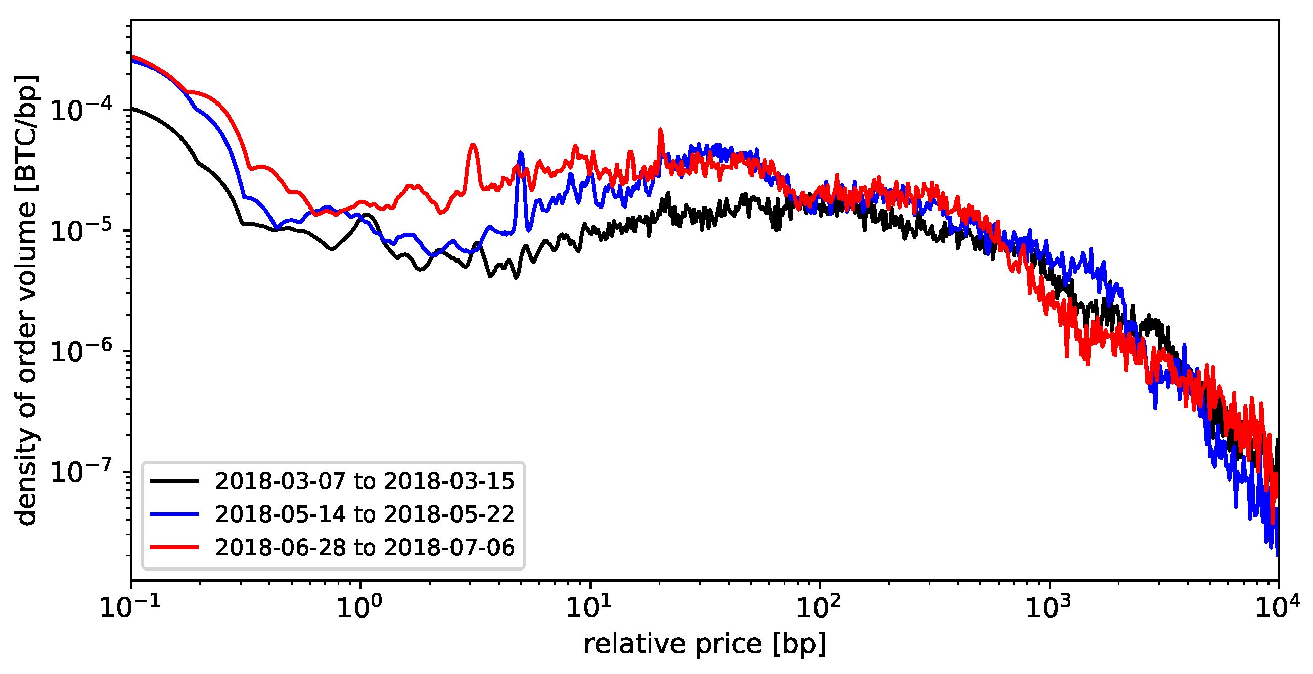
Broad distribution of limit order prices and hump-shaped average order book: Several authors have reported empirical time-averaged limit order volumes as a function of the price difference to the current bid or ask (see Bouchaud et al. (2002), Potters and Bouchaud (2003) and Gu et al. (2008)). Figure 4 presents the density of limit order depth $\overline{q_i^a}$ (or $\overline{q_i^b}$) as a function of relative price $\tilde{p}$ (Figure 4), which we estimate using a kernel density estimator with bandwidth $0.25bp$. We identify the following main characteristics:

• Global maximum at (best) bid and ask: Consistent with the findings from the time-averaged cumulated depth profile, we find the global maximum of volume at the current bid or ask of the LOB. This structure resembles the finding by Potters and Bouchaud (2003) for the SPY exchange-traded fund at Island ECN, where maximum limit order volume is found at the best bid and ask.
• Maximum away from current price: There is a second, local maximum further away from the current bid (or ask), which we locate at relative prices in the order of $\tilde{p}\approx$ 1%. We find the location of this maximum to be roughly symmetric between the ask and bid side of the order book. Both Bouchaud et al. (2002) and Gu et al. (2008) report a maximum in the average shape of the LOB located several ticks deep in the order book, yielding a hump-shaped average order book. In contrast to data from the Bitcoin exchange, this maximum is in relation closer to the current price.
• Bouchaud et al. (2002, Broad distribution of time-averaged volume:) find that orders are placed as far as 50 percent away from the current mid price; however most limit order volume is located within the first 100 ticks surrounding the current price, consistent with the analyses of Potters and Bouchaud (2003) and Gu et al. (2008). In contrast, we find a very broad distribution of volume around the current mid price, which extends with significant shares of the total limit order volume to up to 100 percent of the current mid price, and for the case of ask orders even further.

To gain a better understanding of our results, we refer to the work by Roşu (2009), who models the hump-shaped volume distribution as an equilibrium: On the one hand, traders are optimistic that limit orders placed away from the current price will eventually execute at a favorable price. On the other hand, they fear that limit orders too far away from the current price will never be executed. Following this picture, there seems to be a pronounced optimism in Bitcoin markets that limit orders far away from the current price will eventually match, which may seem likely for market participants in the light of highly volatile prices. In addition, Bitcoin markets do not close during night, and limit orders can have unlimited lifetime, leading to significant limit order volume at highly speculative prices far away from the current mid price. Bitcoin markets are unregulated, with exchanges, to our knowledge, not imposing any restrictions that limit orders need to be placed within a fixed bandwidth around the current mid price. This stands in contrast to more mature markets, where such conditions may be imposed—see Interactive Brokers (2019). The observed second local maximum might therefore correspond to the hump observed in other markets, but much further away from the current price.

Robustness checks: The general shape of the average limit order depth is similar for different subperiods of data (compare Figure 4). Results from other exchanges are generally consistent with these results.

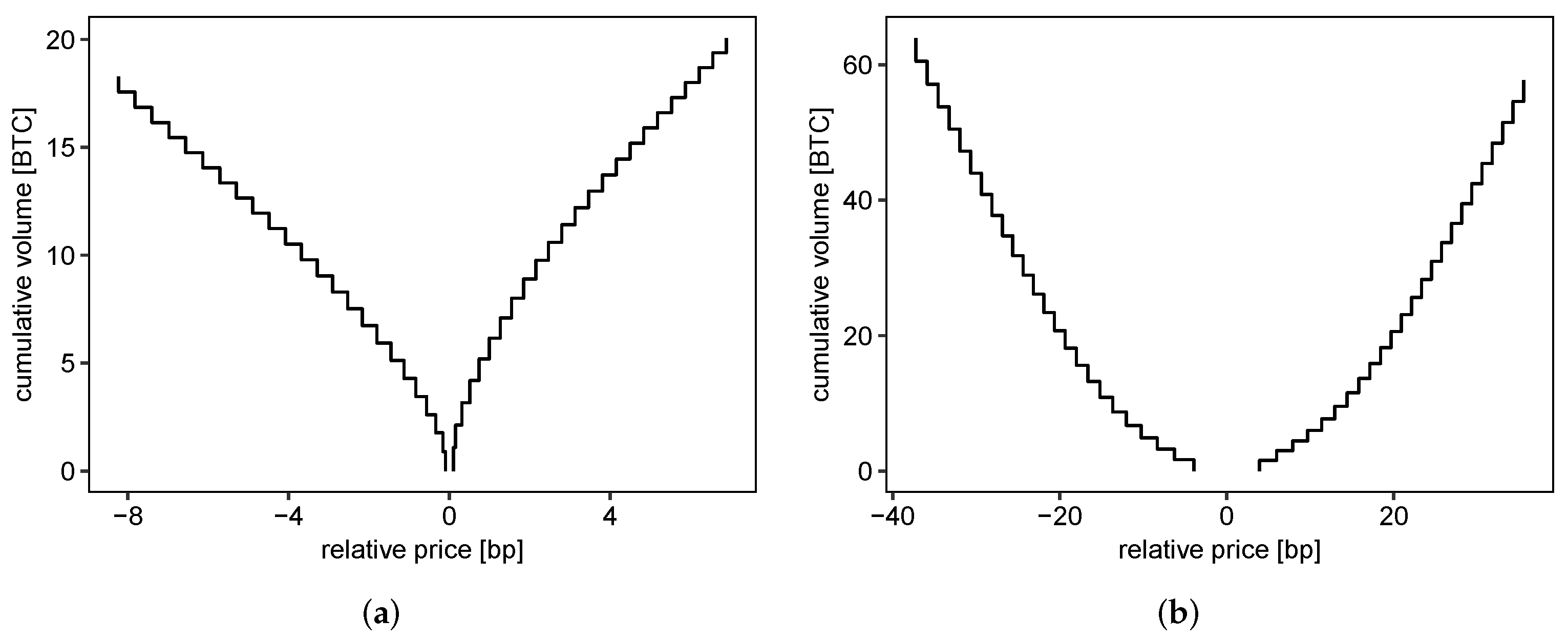
Liquidity costs: Knowledge of the full depth profile of the LOB at any time t allows to determine the liquidity premium for the virtual immediate execution of a market order of size $\left|\omega \right|$. This is particularly interesting since liquidity costs make up an important part of transaction costs, which are critical, e.g., for the profitability of high-turnover statistical arbitrage strategies.

Table 5. Descriptive statistics of liquidity cost measures. We list descriptive statistics of the bid-ask spread $\tilde{s}$ and volume-weighted average price spreads $\widetilde{vs}$ for different order volumes $\omega$.

		$\mathit{\omega }$ [BTC]						$\mathit{\omega }$ [USD]
	$\tilde{\mathit{s}}$	0.1	0.5	1.0	2.0	5.0	10.0	${10}^5$	${10}^6$
min	0.1000	0.1000	0.1000	0.1000	0.1000	0.1000	0.1000	0.1000	0.1291
max	327.2825	327.2825	327.2825	327.2825	327.2825	327.7916	330.2782	327.9760	381.7934
mean	0.9663	1.1993	1.6364	2.0350	2.7790	4.8564	7.8754	8.3667	39.6270
sd	2.4048	2.6776	3.1408	3.5267	4.1727	5.7297	7.6235	6.7230	14.9090
q25	0.1350	0.1405	0.1488	0.1520	0.1604	1.0064	2.9504	4.0599	31.2217
q50	0.1554	0.1591	0.4497	0.7421	1.2843	3.2525	5.8831	7.0778	37.0837
q75	0.8783	0.9870	1.8381	2.5691	3.7175	6.5002	10.2739	10.8947	45.1485
skew	17.0203	13.9014	10.0866	8.2406	6.4527	4.2931	3.2508	3.4022	2.6558
kurt	1201.9088	831.4204	465.3095	309.4683	183.0332	74.8028	37.9242	49.7824	17.6048

reports descriptive statistics of the VWAP spread7 $\widetilde{vs}(\omega ,t)$ for different volumes $\omega$ and the bid-ask spread $\tilde{s}$.

We find an average bid-ask spread of 0.97 bp with a distribution skewed towards lower bid-ask spreads (median spread of 0.16 bp, skewness ≈ 17). For a similar time period but different exchanges, Dyhrberg et al. (2018) find comparable average quoted bid-ask spreads ranging from 0.54 bp to 7.8 bp and point out that these are “significantly lower than the average quoted (effective) spread [...] of stocks on the NYSE” (Dyhrberg et al. 2018, p. 141). However, taking into account liquidity deeper into the order book, we find that liquidity costs rise fast for larger volumes $\omega$: Two-sided VWAP spreads for 1 BTC are on average twice as high as the bid-ask spread, and rise by roughly one order of magnitude (8.37 bp) for a volume of ${10}^5$ USD, which still is a relatively small amount for traditional institutional investors. When compared to a similar analysis by Gomber et al. (2015), the depth of the LOB beyond the best bid or ask is limited: For DAX stocks, the ratio between liquidity costs for ${10}^6$ EUR and the bid-ask spread is between 5 and 12, whereas we find a value of roughly 41.

Robustness checks: When considering subperiods of data, we find that average liquidity costs for small volumes depend on the current market phase (also compare Section 5.1.2). In SP1, liquidity is on a generally higher level, but the scaling of liquidity costs with volume is similar. The scaling of liquidity costs with volume is even more extreme for the second largest exchange (Coinbase): With 0.20 bp, the bid-ask spread is narrower on average (compare

Table A3. Descriptive statistics of liquidity cost measures for the Coinbase (panel A) and the Bitstamp BTC/USD market (panel B). We list descriptive statistics of the bid-ask spread $\tilde{s}$ and volume-weighted average price spreads $\widetilde{vs}$ for different order volumes $\omega$.

			$\mathit{\omega }$ [BTC]						$\mathit{\omega }$ [USD]
		$\tilde{\mathit{s}}$	0.1	0.5	1.0	2.0	5.0	10.0	${10}^5$	${10}^6$
A	mean	0.1984	0.4565	0.8852	1.2585	1.9590	3.9038	6.9085	8.2644	55.9732
	sd	18.8463	1.6903	3.0141	2.7074	3.3185	4.6643	6.2279	6.4667	72.2166
	q25	0.0112	0.0116	0.0121	0.0124	0.0137	0.2657	2.5405	3.7401	42.1128
	q50	0.0133	0.0142	0.0150	0.0155	0.3297	2.6565	5.7849	7.4037	51.9763
	q75	0.0152	0.0157	0.4227	1.3888	2.8715	5.7636	9.5908	11.4203	63.9471
	skew	208.2537	9.5766	173.4533	5.0151	3.9150	2.8447	2.3831	2.0350	129.3065
	kurt	43464.80	228.58	69382.36	63.09	37.55	19.99	14.23	12.14	21011.61
B	mean	7.8612	9.0643	10.5030	11.6672	13.7398	18.2892	23.5749	24.9565	73.5508
	sd	7.3941	7.9357	8.7012	9.3081	10.0856	11.6074	13.0441	11.7406	21.6807
	q25	2.6739	3.6618	4.7017	5.4402	6.9664	10.7988	15.4833	17.8222	58.9856
	q50	6.3022	7.4225	8.6849	9.6938	11.7622	16.0878	20.7755	22.8481	69.9553
	q75	10.7758	12.2041	13.8400	15.1248	17.3629	22.0618	27.1251	28.6737	83.7376
	skew	2.2649	2.1057	2.0129	1.9788	1.9183	1.8158	1.7826	1.7740	1.7231
	kurt	17.3872	14.8690	11.7922	10.3188	8.9804	6.9622	5.8785	7.1700	7.5178

), which might be a consequence of the smaller price increment of 0.01 USD. However, liquidity costs rise fast, and assume values similar to the BitFinex exchange for larger volumes. The ratio between liquidity costs for ${10}^6$ USD and the bid-ask spread is at 282.

5.1.2. Time Series Characteristics of Statistics

We now turn to the study of time series properties of selected measures of the static LOB.

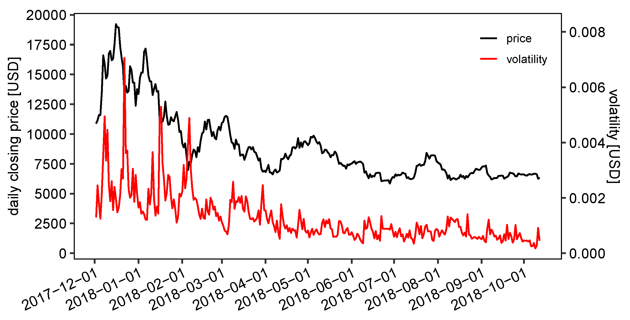
Non-normal return distribution:Figure 5 displays the evolution of the last mid-price $m\left(t\right)$ of the day, as well as the daily realized volatility (Equation (7)). Besides the expected non-stationarity of this time series, we observe high volatility with double-digit percentage price changes during the first months of our data. This picture is reinforced by the descriptive statistics of mid-price returns $r^{mid}(t,\Delta t)$ in

Table 6. Descriptive return statistics. This table lists statistical properties of logarithmic mid-price returns $r^{mid}(t,\Delta t)$ on different time scales $\Delta t$, in units of 1 bp (where applicable).

	$\Delta \mathit{t}=1\mathbf{min}$	$\Delta \mathit{t}=1\mathbf{h}$	$\Delta \mathit{t}=1\mathbf{day}$
min	−363.0070	−1273.4918	−2039.0606
max	454.4009	1127.3911	2063.1761
mean	−0.0219	−0.6505	−15.1541
sd	15.3572	115.6858	497.8412
q25	−3.4865	−35.9549	−232.2230
q50	0.0000	1.2460	5.8898
q75	3.5754	35.1836	187.2999
skew	0.1583	0.0309	−0.0797

, for different time scales $\Delta t$. Both positive and negative daily logarithmic returns have extremal values close to 20 percent. Median and mean returns are close to zero. Daily returns are slightly skewed to the left, minutely returns are slightly skewed to the right.

Next, we will evaluate the tail index estimates.

Table 7. Analysis of tails of the return distribution. This table shows measures for the tails of the distribution of logarithmic mid-price returns on different time scales $\Delta t$. We use kurtosis metrics based on the fourth standardized moment ($m_4^e$) and based on quantiles (${\gamma }_{p=0.025,q=0.125}^e$), as well as tail indices from a Hill estimator ($H_p$). The measures are applied to the full distribution as well as to the left and right side of the distribution only. SP1 and SP2 refer to subperiods of data.

	SP1 and SP2						SP1		SP2
$\Delta \mathit{t}$	$\mathbf{1}\mathbf{min}$			$\mathbf{1}\mathbf{h}$			$\mathbf{1}\mathbf{min}$	$\mathbf{1}\mathbf{h}$	$\mathbf{1}\mathbf{min}$	$\mathbf{1}\mathbf{h}$
Side	Both	Left	Right	Both	Left	Right	Both	Both	Both	Both
$m_4^e$	44.3497	41.5939	47.3472	17.6771	18.0461	17.3392	32.219	11.6763	77.9707	30.7078
${\gamma }_{p=0.025,q=0.125}^e$	0.6481	0.7975	0.6004	0.5784	0.4773	0.6922	0.3992	0.2830	0.5555	0.9727
$H_{p=10\%}$	2.0521	1.9382	2.1681	2.2681	2.4375	2.1438	2.4160	2.6743	2.0854	1.8972
$H_{p=5\%}$	2.4823	2.3919	2.5650	2.8674	2.8448	2.8233	2.8642	3.2549	2.3750	2.1826
$H_{p=2.5\%}$	2.8954	2.8852	2.9079	3.2968	3.6668	2.9610	3.2203	3.7743	2.4933	2.7144

summarizes the results of the tail analysis for minutely and daily data. For the Hill estimator $H_p$ (Equation (11)) to be meaningful, approximately 2000 observations are needed (Lux and Marchesi 2000), and we therefore do not show Hill estimates for daily data (313 observations). Our tail index estimates range between 1.94 and 3.67, which is in line with the literature. Smaller estimates indicate heavier tails. Estimates for the tail index smaller than four are associated with infinite fourth moments making $m_4$ unreliable. Thus, we show excess kurtosis values $m_4^e$ but do not interpret them. A typical pattern for stocks can also be found in our context, namely that the tail index estimator increases with the number of observations considered as being in the tails (Lux and Marchesi 2000). Our results provide evidence that mid returns exhibit heavy tails, i.e., the probability of extreme events is higher compared to a normal distribution. For the case where we do not distinguish between the two tails of the distribution (columns “both”), this can be seen from the quantile-based excess kurtosis metric ${\gamma }_{p=0.025,q=0.125}^e$ close to 0.6.8 The Hill estimates between 2.05 and 2.90 ($\Delta t=1\min$) as well as 2.27 and 3.30 ($\Delta t=1\mathrm{h}$) point into the same direction. According to both metrics, we can draw the following further conclusions: First, minute data have heavier tails than hourly data, i.e., excess kurtosis values are larger, and Hill estimates smaller. Second, the left tail is heavier than the right tail for minute data and vice versa for hourly data. The latter holds true independent of the number of observations declared as tail. In a recent contribution, Zhang et al. (2018) use the $m_4$ kurtosis metric and the Hill estimator to analyze the tails of eight cryptocurrencies, among them Bitcoin. For two years of daily returns, computed from closing prices, the authors point out that all examined cryptocurrencies exhibit heavy tails. Overall, we can reproduce the stylized facts on the empirical distribution of returns as summarized by Cont (2001): The distribution of mid-price returns has a sharp peak centered around zero and exhibits fat tails, and is therefore insufficiently described by the normal distribution.

Robustness checks: We recalculate tail measures for subperiods of the data (columns “SP1” and “SP2” in Table 7). The patterns for SP1 are in line with those observed for the SP1 and SP2. Also, we find similar tail patterns when comparing results to those obtained for the Coinbase and Bitstamp exchange.

Autocorrelation of returns and volatility clustering: We check the common fact that “price movements in liquid markets do not exhibit any significant autocorrelation” (Cont 2001, p. 229), and compute the autocorrelation function of mid-price returns $C^{mid}\left(n\right)$ on different time scales (

Table 8. Autocorrelation of logarithmic, absolute and squared returns. We compute the autocorrelation functions $C^{mid}\left(n\right)$, $C_1^{mid}\left(n\right)$ and $C_2^{mid}\left(n\right)$ for different lags n, different time scales $\Delta t$ and different subperiods.

		$\Delta \mathit{t}=1\mathbf{min}$			$\Delta \mathit{t}=1\mathbf{h}$			$\Delta \mathit{t}=1\mathbf{day}$
	lag n	${\mathit{C}}^{\mathit{mid}}\left(\mathit{n}\right)$	${\mathit{C}}_2^{\mathit{mid}}\left(\mathit{n}\right)$	${\mathit{C}}_1^{\mathit{mid}}\left(\mathit{n}\right)$	${\mathit{C}}^{\mathit{mid}}\left(\mathit{n}\right)$	${\mathit{C}}_2^{\mathit{mid}}\left(\mathit{n}\right)$	${\mathit{C}}_1^{\mathit{mid}}\left(\mathit{n}\right)$	${\mathit{C}}^{\mathit{mid}}\left(\mathit{n}\right)$	${\mathit{C}}_2^{\mathit{mid}}\left(\mathit{n}\right)$	${\mathit{C}}_1^{\mathit{mid}}\left(\mathit{n}\right)$
SP1 and SP2	1	0.0342	0.2847	0.4667	−0.0722	0.1625	0.2962	0.0004	0.1443	0.1209
	2	−0.0172	0.2357	0.4295	0.0134	0.2028	0.3259	0.0179	0.0436	0.1205
	3	−0.0055	0.2198	0.4121	−0.0208	0.1690	0.3071	0.0107	0.0766	0.1681
	4	−0.0015	0.2324	0.4041	−0.0364	0.1366	0.2833	−0.0862	0.2132	0.1960
	5	−0.0074	0.2069	0.4005	−0.0083	0.2034	0.3264	0.0441	0.0796	0.1203
	6	−0.0093	0.2112	0.3961	0.0212	0.1386	0.2850	0.0174	0.0887	0.1428
	7	−0.0169	0.1976	0.3885	−0.0120	0.1785	0.3083	−0.0201	0.0733	0.1395
	8	−0.0097	0.1858	0.3835	0.0071	0.2399	0.3399	0.0531	0.1511	0.2352
	9	−0.0068	0.1873	0.3784	−0.0427	0.2007	0.3056	−0.0229	0.0528	0.0892
	10	−0.0055	0.1944	0.3801	0.0535	0.2099	0.2927	−0.0307	0.1126	0.1503
SP1	1	0.0306	0.2706	0.4019	−0.0900	0.1324	0.2084	−0.0044	0.0678	−0.0331
	2	−0.0186	0.2267	0.3683	0.0170	0.1793	0.2588	0.0071	−0.0532	−0.0188
	3	−0.0066	0.2119	0.3523	−0.0256	0.1432	0.2421	0.0116	−0.0107	0.0539
	4	−0.0001	0.2265	0.3452	−0.0403	0.1067	0.2109	−0.1007	0.1495	0.0927
	5	−0.0080	0.1995	0.3432	−0.0098	0.1822	0.2663	0.0533	0.0075	0.0164
SP2	1	0.0592	0.2883	0.3813	0.0157	0.0757	0.1497	0.0189	−0.0040	0.0720
	2	−0.0076	0.1446	0.2933	−0.0162	0.0029	0.0512	0.0613	0.0169	0.0044
	3	0.0019	0.1071	0.2538	−0.0005	0.0342	0.0651	−0.0042	−0.0530	−0.0213
	4	−0.0112	0.0914	0.2339	0.0019	−0.0044	0.0359	−0.0424	−0.0098	−0.0080
	5	−0.0033	0.0810	0.2190	−0.0035	−0.0073	0.0292	0.0132	−0.0785	−0.0848

): We find a small positive autocorrelation of 0.0343 on the minute time scale for a lag of one minute. Turning to daily data, we do not find significant structure in the autocorrelation, which is confirmed by the Ljung-Box test (Ljung and Box 1978) with the null hypothesis of no autocorrelation.9

On the other hand, nonlinear functions of returns are known to show significant autocorrelation, which is referred to as volatility clustering (Cont 2001). As for a wide range of other markets, we find that the autocorrelation of squared returns is positive and decays slowly with the lag n. Following several other authors, we fit a power law $C_2^{mid}\left(n\right)\sim n^{-\beta }$ and obtain coefficients of $\beta \approx 0.16$ and $\beta \approx 0.24$ for the decay of autocorrelation on the minutely and hourly time scale, respectively, which is at the lower end of the range given by Cont (2001) ($\beta \in [0.2,0.4]$). The effect size of autocorrelation in squared and absolute returns decreases with the frequency. For absolute and squared daily returns, we test the null hypothesis of no autocorrelation using the Ljung-Box test (Ljung and Box 1978), which we can reject (p-value of 0.0000). Our findings for daily data are in line with Zhang et al. (2018). The authors report for all eight analyzed cryptocurrencies that autocorrelation decays at a fast rate for returns and slowly for absolute returns. In addition, they found significant volatility clustering.

Robustness checks: The subperiod analysis for SP1 and SP2 (panels “SP1” and “SP2” in Table 8) reveals that the general results for the full time period carry over to the subperiods. When comparing results with other exchanges, we obtain a similar picture.

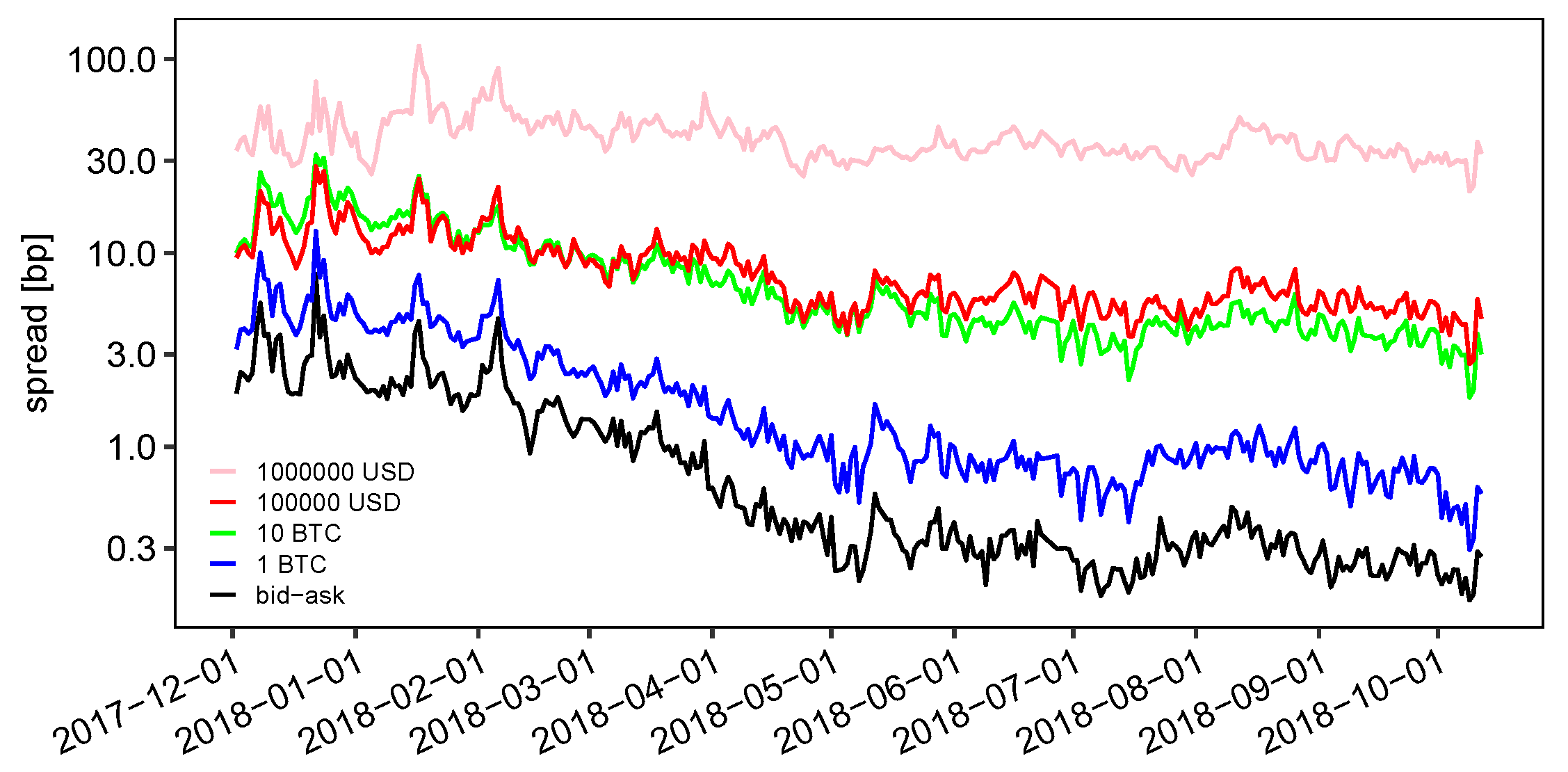
Evolution of liquidity costs:Figure 6 displays the evolution of the daily averages of the relative bid-ask spread $\tilde{s}\left(t\right)$ and the VWAP spread $\widetilde{vs}(\omega ,t)$ for virtual market orders of different sizes $\omega$. We make the following observations: First, the bid-ask spread $\tilde{s}\left(t\right)$ varies over approximately one order of magnitude from 3 bp in late 2017/early 2018 to roughly 0.3 bp after May 2018. This stark change is in line with the evolution of the average weekly bid-ask spread for several Bitcoin exchanges found by Dyhrberg et al. (2018). Second, we find that the variation in the level of liquidity costs for higher volumes is less pronounced: For example, the VWAP spread $\widetilde{vs}(\omega ,t)$ for a value of ${10}^6$ USD remains—in relation to the bid-ask spread—closer to the long-term average value of 39.62 bp. Third, the analysis shows that the costs of liquidity provision are higher in times of high Bitcoin price and high volatility: The linear correlation coefficients between the daily closing price are $\rho \approx 0.73$ for the bid-ask spread and $\rho \approx 0.21$ for the VWAP spread for ${10}^6$ USD.

Robustness checks: We find that results from the exchanges Coinbase and Bitstamp exhibit a similar evolution of liquidity cost measures (compare Figure A2 in the Appendix A).

5.1.3. Conditional Statistics of the Limit Order Book

Finally, we present two selected analyses based on conditional statistics of measures of the static LOB, namely intraday patterns of liquidity costs and liquidity resiliency.

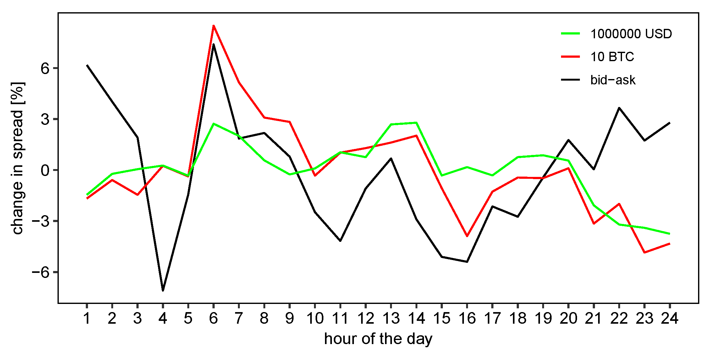
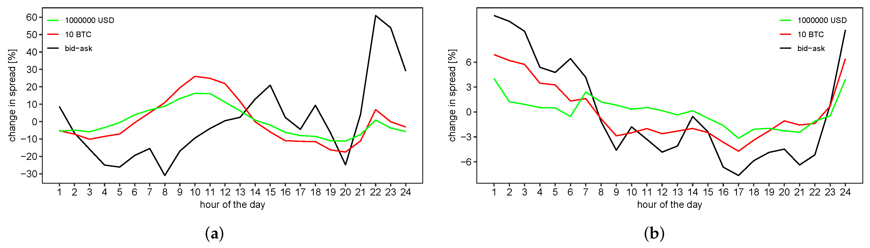
Intraday patterns of liquidity costs: A common result for limit order markets is that the bid-ask spread has a U-shaped intraday pattern: McInish and Wood (1992) find for NYSE data that averaged bid-ask spreads are highest at the beginning and the end of the trading day. Similar results have been obtained for a foreign exchange market (Danielsson and Payne 2001), the Swiss Stock Exchange (Ranaldo 2004) and the Paris Bourse (Biais et al. 1995). Gomber et al. (2015) demonstrate that VWAP spreads are approximately doubled near the start and end of the continuous trading session for Xetra-traded DAX stocks. Figure 7 displays the change of the average hourly distribution of the bid-ask spread $\tilde{s}\left(t\right)$ and liquidity costs $\widetilde{vs}(\omega ,t)$ for 10 BTC and ${10}^6$ USD relative to the mean value at the BitFinex BTC/USD market. We observe that average liquidity cost measures vary only slightly across the day (with relative changes of a few percent) with no clearly visible pattern. Dyhrberg et al. (2018, 10) make the same observation for averaged bid-ask spreads from three Bitcoin markets and attribute this to the continuous trading at every hour of the day at cryptocurrency markets. In addition, we conjecture that these results could be explained by a worldwide market participation leading to a superposition of intraday patterns from different time zones and the presence of automated trading, such that no clear picture can emerge.

Robustness checks: As expected, the observed average hourly changes in liquidity are not robust when considering subperiods of data, which supports the conclusion of absent intraday patterns. We find a clear but weak U-shaped intraday pattern in liquidity costs for the Bitstamp exchange (compare Figure A3 in the Appendix A), which could be due to a focus of trading activity on the European market.11 In contrast, we observe larger variations at the Coinbase exchange, but no universal pattern emerges when comparing bid-ask spread and liquidity costs for higher volumes. Overall, we observe a mixed picture: Hourly average liquidity costs differ largely between cryptocurrency exchanges, and pronounced patterns known from established markets are largely absent.

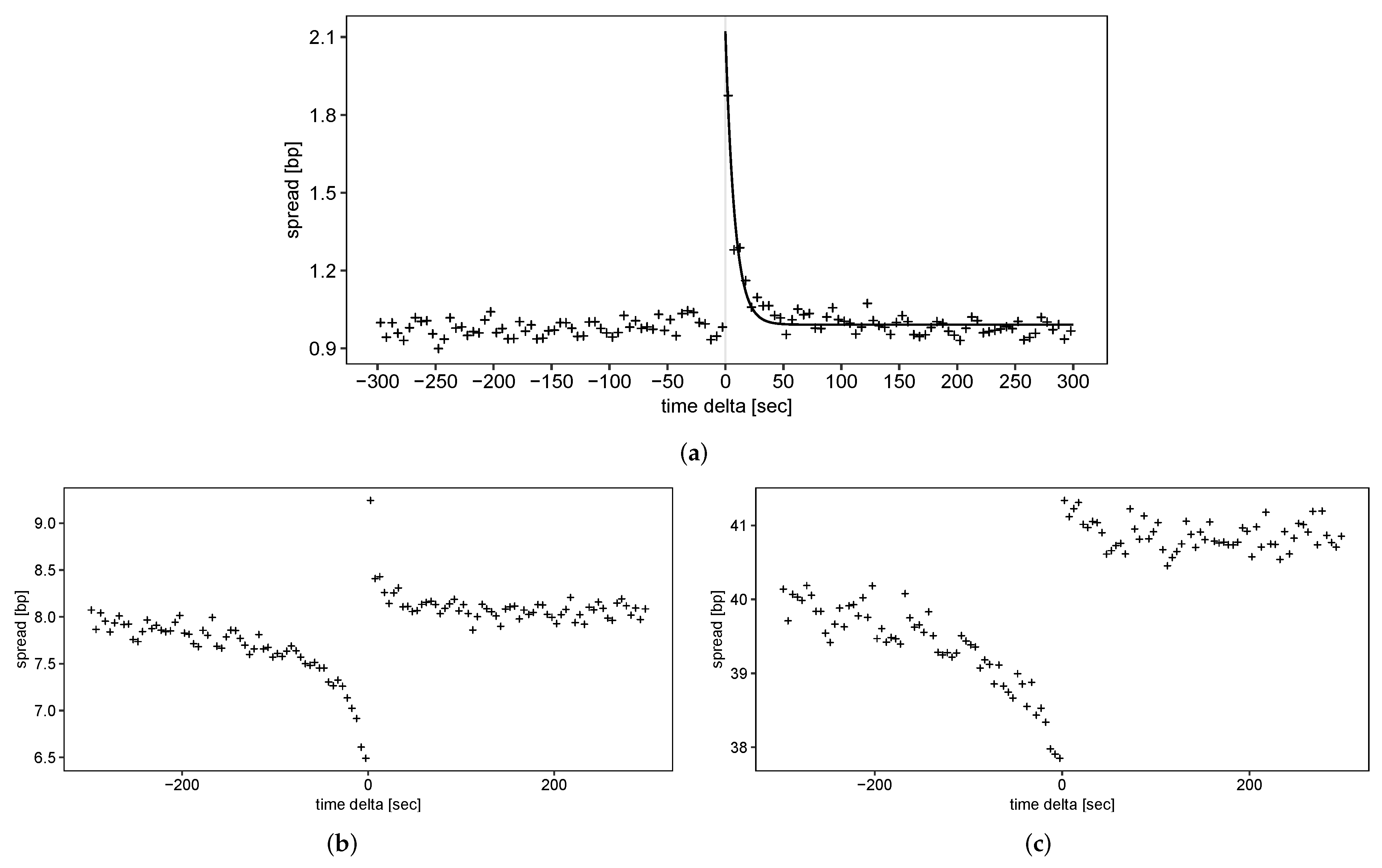
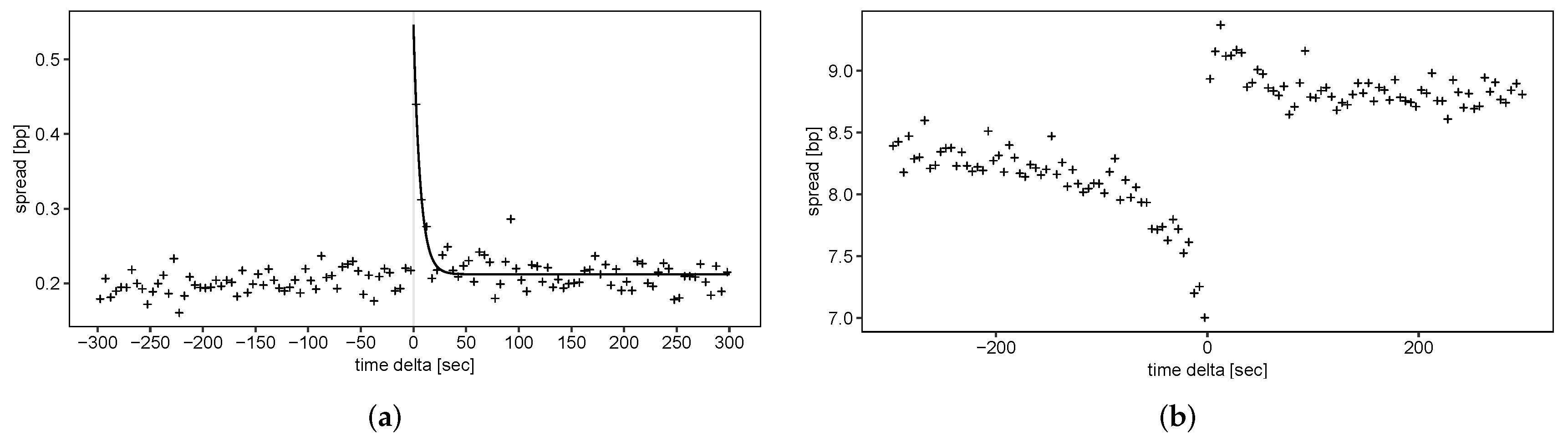
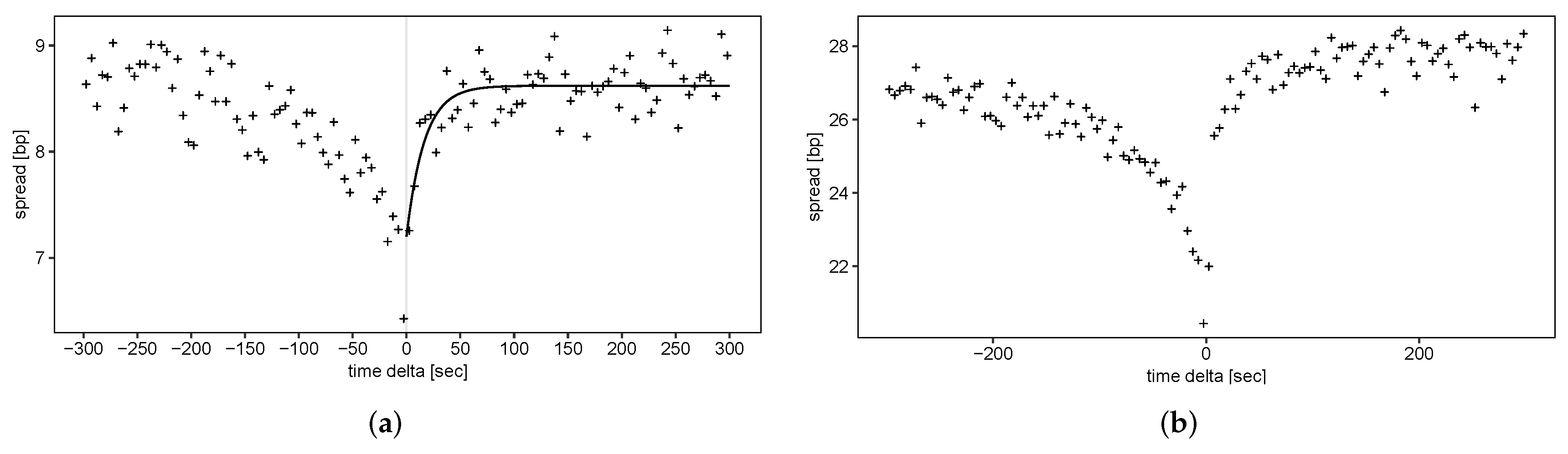
Liquidity resiliency and timing of large trades: We now characterize the recovery of limit order liquidity after liquidity shocks, and analyze whether large trades are timed in the sense that they occur when liquidity is high. We examine average liquidity costs (precisely, the relative bid-ask spread $f=\tilde{s}$ and VWAP spread $f=\widetilde{vs}$) as a function of the event time $\tau$ in temporal vicinity of large trades (Equation (12)). We consider the one percent largest trades ($N=$ 510,584) to obtain sufficient statistics. Figure 8 displays results for the bid-ask spread and the VWAP spreads for ${10}^5$ USD and ${10}^6$ USD. Compared to relevant literature, we make the following observations:

• Recovery of the bid-ask spread: We first consider the typical speed at which liquidity recovers after a large trade. We find that the average bid-ask spread increases to roughly 2 bp directly following the trade and subsequently recovers to its pre-event value of about 1 bp (Figure 8a). We fit an exponential decay function $\overline{s}\left(\tau \right)\sim exp(-\tau /T)$ to estimate the decay time constant as $T\approx 8.3$ s (corresponding to a half-life of $T_{1/2}\approx 5.8$ s). Surprisingly, this is well in line with the finding of Cummings and Frino (2010) for large block trades of interest rate futures at the Sydney Futures Exchange: Considering only the largest block trades, they find that excess bid-ask spreads after the largest block purchases recover to a normal level on a time scale of approximately 7 s. They find that recovery is faster for the largest trades. Similarly, Large (2007) estimates a half-life time of about 20 s for a stock at the London Stock Exchange.
• Recovery of liquidity beyond the (best) bid and ask: For liquidity provided from deeper levels of the LOB, we find that liquidity does not quite recover to pre-event levels in the considered time window of 300 s (compare Figure 8b,c). Gomber et al. (2015) find that “it takes longer to restore large depth than to restore a small spread” (Gomber et al. 2015, p. 67). They estimate that it takes about four minutes to restore liquidity costs for ${10}^5$ EUR. For similar volumes (Figure 8b) we observe that average liquidity after the trade still differs slightly from pre-trade values.
• Pre-trade liquidity increase and timing of large transactions: For average liquidity costs for ${10}^5$ USD and ${10}^6$ USD, we find—at first quite surprisingly—that liquidity increases prior to a large trade. This effect is observed in time windows of 2–3 min preceding the trade. Gomber et al. (2015) report a very similar finding for the evolution of the average exchange liquidity measure: Liquidity costs for ${10}^5$ EUR and DAX stocks decrease over an interval of about three minutes before large trades. Noticing that the increase in liquidity takes place on the side of the market where the trade occurs, they interpret this effect in terms of timed large transactions: Market participants prefer to execute large trades when liquidity is exceptionally high, and the execution of large trades relatively cheap. Our results indicate that the timing of large transactions is also present in Bitcoin markets.

Robustness checks: We obtain similar results for subperiods SP1 and SP2 of our data. To check that results are not driven by clusters of trades, we follow Gomber et al. (2015) and redo calculations for all large trades that are not followed by other large trades within 15 min. We observe very similar results and conjecture that our results are not dominated by the clustering of trades. When comparing results to the exchange Coinbase (compare Figure A4 in the Appendix A), we observe similar patterns in the recovery of liquidity. However, results are different for the smallest exchange in our sample (Bitstamp), where we observe an increase of liquidity costs after the trade. These results could be due to a market maker or some other idiosyncrasy of the exchange, for example the generally lower liquidity or differences in trade and order sizes.

5.2. Analysis of the Dynamics of the Limit Order Book: Order and Trade Flows

5.2.1. Unconditional Descriptive Statistics of Trades and Order Book Changes

We next present unconditional descriptive statistics of measures of the dynamic LOB, i.e., properties of trades and the limit order flow, and begin by discussing the distribution of trade size.

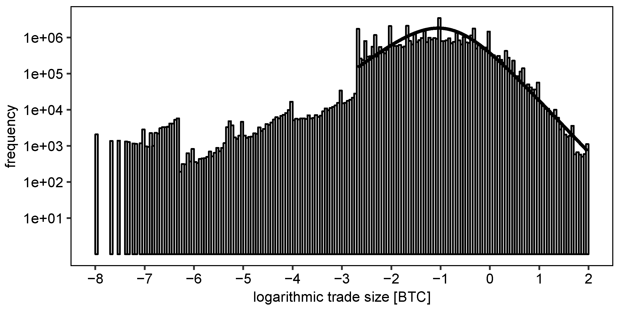
Distribution of trade size:

Table 9. Descriptive statistics of trades. This table lists descriptive statistics of the price $p_M$, the value ${\omega }_M·p_M$ and the size ${\omega }_M$ for all trades.

	${\mathit{p}}_{\mathit{M}}$ [USD]	${\mathit{\omega }}_{\mathit{M}}·{\mathit{p}}_{\mathit{M}}$ [USD]			${\mathit{\omega }}_{\mathit{M}}$ [BTC]
	All	All	Ask-Initiated	Bid-Initiated	All	Ask-Initiated	Bid-Initiated
count	51,058,356	51,058,356	26,112,746	24,945,610	51,058,356	26,112,746	24,945,610
mean	8665.11	3053.87	3059.75	3047.72	0.3643	0.3658	0.3627
sd	2493.81	13,658.82	14,155.62	13,118.64	1.6686	1.7441	1.5857
q25	6710.00	138.14	134.45	143.19	0.0170	0.0160	0.0180
q50	8011.30	634.33	626.23	641.15	0.0752	0.0748	0.0760
q75	9602.40	2431.44	2419.27	2440.93	0.2938	0.2906	0.2970
skew	1.52	89.51	97.32	78.79	94.84	92.21	97.75

lists descriptive statistics of the price $p_M$ and size ${\omega }_M$ of all trades in our sample ($N=$ 51,058,356). There seems to be a large amount of retail trading: With a median trade value of roughly 634 USD (0.0752 BTC), most trades are comparably small. Figure 9 displays the rich structure in the distribution of trade size ${\omega }_M$, for which we observe the following:

• Two regimes separated by the minimum order size: The distribution of trade size exhibits a large jump at the minimum order size of 0.002 BTC, and separates two regimes: For smaller trades, trade frequency increases with trade size, but exhibits discontinuities. For larger trade sizes, the distribution exhibits a convex plateau and a power tail for trades larger 1 BTC.
• Power-law dependence of volume for large trades: For trade sizes exceeding the minimum order size, the empirical distribution of trade size agrees well with results from the literature: Similar to the results of Mu et al. (2009), the empirical distribution of trade sizes larger than the minimum order size fits well to a q-Gamma distribution $p\left({\omega }_M\right)\propto {\left({\omega }_M\right)}^{\beta }{\left[1-(1-q)\frac{{\omega }_M}{\theta }\right]}^{{(1-q)}^{-1}}$ with parameters $\beta \approx {10}^{-4}$, $\theta \approx 5.28·{10}^{-2}$ and $q\approx 1.41$. The asymptotic tail exponent of this distribution is given by $\alpha =\frac{1}{q-1}-\beta -1\approx 1.44$. Gopikrishnan et al. (2000) and Maslov and Mills (2001) find power tails with comparable values for US stock markets ($\alpha =1.53\pm 0.07$) and the NASDAQ ($\alpha =1.4\pm 0.1$).
• Significant share of trades smaller than the minimum order size: A large share of trades has a size smaller than the minimum order size. We interpret these results in the light of a minimum order size increment (${10}^{-8}$ BTC) much smaller than the minimum order size (0.002 BTC), leading to trade sizes much smaller than the minimum order size. For example, an ask order with initial volume 0.0021 BTC could be partially matched with a bid order of 0.002 BTC, leaving a small ask order active that could subsequently lead to a trade of size 0.0001 BTC.
• Mu et al. (2009, Number preference:) reported that traders seem to prefer certain numbers for order sizes, which also manifests in the distribution of trade size. Similarly, we observe peaks in trade frequency for certain sizes, for example at 0.01 BTC, 0.02 BTC, 0.1 BTC, 0.5 BTC and 1 BTC.

Contrary to traditional equity markets investigated in the literature, minimum order size and the order size increment differ largely for cryptocurrency markets due to the divisibility of Bitcoin, leading to the observation a different trade size distribution.

Robustness checks: The shape of the empirical distribution of trade size is robust with respect to considering subperiods SP1 and SP2 of our data. We obtain very similar empirical distributions for the other two exchanges, albeit slightly different minimum order sizes (compare Table 1).

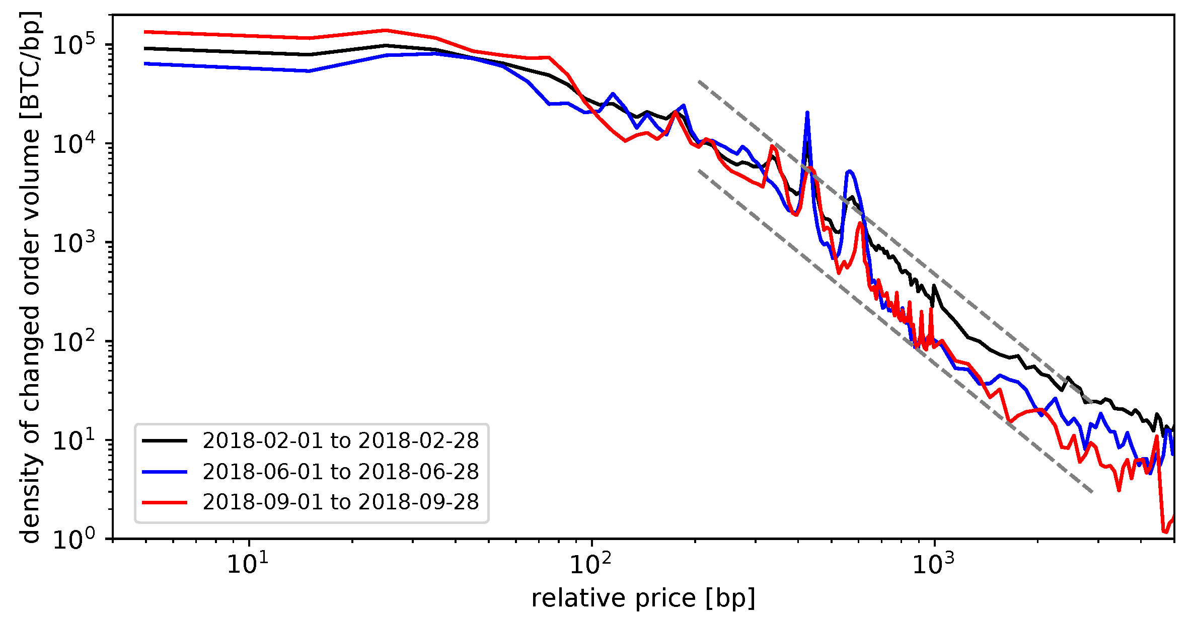
Distribution of changes in limit order depth: Next, we consider the flow of limit order volume to and from the LOB. In Figure 10, we plot the time-averaged empirical density of changed limit order volume in the LOB, i.e., $\overline{\Delta n^b\left(p\right)}$ and $\overline{\Delta n^a\left(p\right)}$ (Equation (14)) on a price scale relative to the current mid price. We make the following observations:

• Power tail away from the current price: Further away from the current mid price, the changed limit order volume declines rapidly. Figure 10 includes dashed straight lines with a slope of roughly −2.8, and the empirical density in log-log axes declines at a roughly similar rate. Power tails in the distribution of order frequency as a function of the difference to the price have been found before (compare, for example, Bouchaud et al. (2002), Zovko and Farmer (2002) and Potters and Bouchaud (2003). These analyses consider all incoming orders, whereas we consider the total change in depth in the LOB. Therefore, a different distribution close to the mid price would be expected.
• Constant changed order volume near the current price: We find a roughly constant density in changed limit order volume up to a relative price of 1 percent. We may cautiously conclude that this finding is still consistent with the literature: Several authors (for example, Bouchaud et al. (2002), Zovko and Farmer (2002) and Potters and Bouchaud (2003)) found that most orders arrive at the current bid or ask price. These orders are, however, executed immediately or with high profitability, and thus cannot be observed in our analysis, leading to the observed plateau in the distribution of changed limit order volume. Orders arriving further away from the current price are less likely executed and lead to persistent changes in limit order depth, which we observe in our analysis.
• Peaked activity away from the current price: Quite surprisingly, we see distinct peaks in changed order volume at relative prices of 4 and 6 percent. These could be the consequence of speculative order placement or the traders’ preference for certain round order prices.

These results are well in line with the previously found broad distribution of limit order volume (compare Section 5.1.1). Specifically, we conjecture that speculative order placement plays an important role in these markets, which is—in contrast to established markets—not restricted by exchanges or regulators by imposing caps on order prices.

Robustness checks: The distributions of LOB changes for all subperiods in Figure 10 are similar, and we find generally consistent results for the other exchanges.

5.2.2. Time Series Characteristics of Trade Properties

Evolution of trading volume and trade size:Figure 11 displays the evolution of daily averages of the trade size, the number of trades and the cumulated volume (compare Section 4.3.2). We make the following observations: First, both the number of trades and cumulated volume are higher during the phase of comparably high prices. Second, peaks in cumulated volume and trade frequency coincide with peaks in volatility of the mid price (compare Figure 5). Third, the average trade size is relatively stable, and decreases in the high-price phase, which might be a consequence of increased retail trading due to higher interest in cryptocurrencies.

Autocorrelation of trade price changes and sizes: While return time series on time scales of minutes to days do typically not possess any significant autocorrelation, high-frequency return time series are found to have negative autocorrelation at the first lags. This is attributed to the bid-ask bounce, i.e., the oscillation of trade prices between prices of the bid side of the LOB and prices at the ask side (Cont 2001; Russell and Engle 2010).

Table 10. Autocorrelation of trade properties. We compute the autocorrelation functions of trade price changes $C^{tp}\left(n\right)$ and trade sizes $C^{size}\left(n\right)$ for lags $n=1,\cdots ,10$. We show results for all trades, for ask-initiated trades (${\omega }_M>0$) and bid-initiated trades (${\omega }_M<0$) separately.

		${\mathit{C}}^{\mathit{size}}\left(\mathit{n}\right)$			${\mathit{C}}^{\mathit{tp}}\left(\mathit{n}\right)$
	lag n	All	${\mathit{\omega }}_{\mathit{M}}>0$	${\mathit{\omega }}_{\mathit{M}}<0$	All	${\mathit{\omega }}_{\mathit{M}}>0$	${\mathit{\omega }}_{\mathit{M}}<0$
SP1 and SP2	1	0.1225	0.1398	0.1176	−0.1759	−0.0790	−0.0833
	2	0.1045	0.1106	0.1128	−0.0529	−0.0204	−0.0234
	3	0.0926	0.0995	0.0946	−0.0302	−0.0110	−0.0147
	4	0.1092	0.1219	0.1061	−0.0107	−0.0001	−0.0033
	5	0.0743	0.0775	0.0796	−0.0128	−0.0059	−0.0066
	6	0.0893	0.0947	0.0931	−0.0032	0.0059	0.0045
	7	0.0672	0.0728	0.0694	−0.0091	−0.0018	−0.0018
	8	0.0890	0.1013	0.0832	−0.0020	0.0048	0.0036
SP1	1	0.1024	0.1314	0.0854	−0.1775	−0.0787	−0.0831
	2	0.0675	0.0718	0.0773	−0.0532	−0.0204	−0.0236
	3	0.0611	0.0644	0.0665	−0.0294	−0.0101	−0.0140
	4	0.0596	0.0609	0.0671	−0.0111	−0.0006	−0.0042
	5	0.0496	0.0505	0.0580	−0.0114	−0.0044	−0.0054
SP2	1	0.1406	0.1464	0.1513	−0.1378	−0.0834	−0.0871
	2	0.1380	0.1419	0.1501	−0.0468	−0.0207	−0.0205
	3	0.1211	0.1278	0.1239	−0.0483	−0.0276	−0.0276
	4	0.1541	0.1713	0.1469	−0.0024	0.0099	0.0121
	5	0.0965	0.0993	0.1021	−0.0458	−0.0320	−0.0288

lists values of the autocorrelation function of trade price changes $C^{tp}\left(n\right)$ (Equation (15)). We observe negative autocorrelations $C^{tp}\left(n\right)$ in the first lags, and $C^{tp}\left(1\right)\approx -0.18$ is comparable in size with results by Russell and Engle (2010). When looking at sell and buy trades separately, we find that $C^{tp}\left(1\right)$ drops to roughly −0.08, which is consistent with autocorrelations being driven mainly by the bid-ask bounce. Results for the autocorrelation function of trade sizes $C^{size}\left(n\right)$ (Equation (16)) exhibit positive values in the order of 0.12, which does not depend on whether we include all trades or only sell or buy trades.

Robustness checks: We obtain similar results when repeating the analyses for subperiods of data (panels SP1 and SP2 of Table 10). Autocorrelation functions for trade price changes and trade sizes behave similarly for the other Bitcoin exchanges.

5.2.3. Conditional Statistics Across All Trades

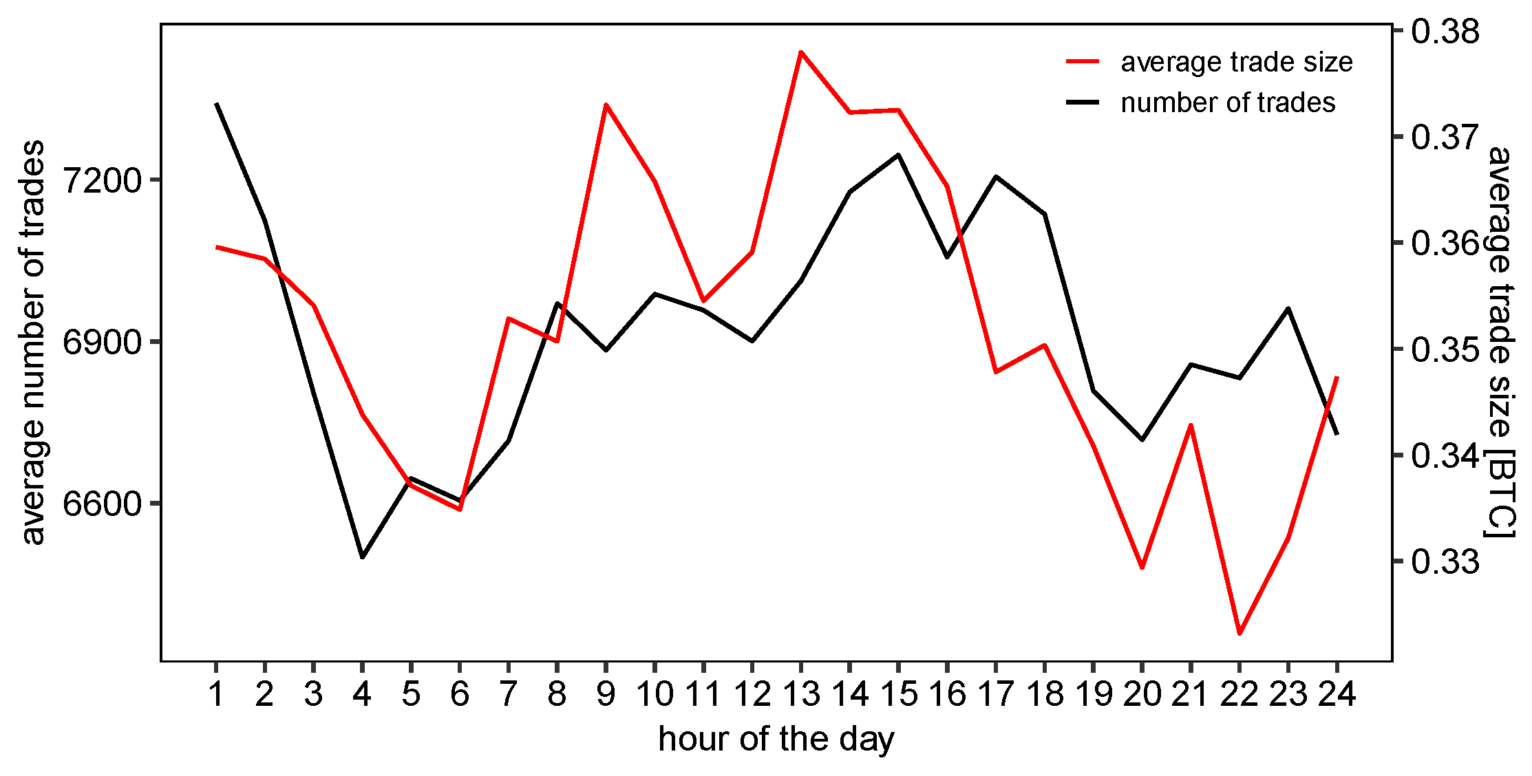
Intraday patterns of trading activity: We now analyze intraday patterns in trading activity. Contrary to commonly found patterns in the bid-ask spread, results from the literature differ depending on the market, and range from U-shaped patterns for stocks at the Paris Bourse (Biais et al. 1995) to M-shaped patterns in data from an FX market (Danielsson and Payne 2001). Figure 12 displays the average trade size and trade frequency conditional on the hour of the day. We make the following observations: First, we find some weakly visible patterns and a similarity between the average trade size ${\omega }_M$ and the number of trades. Second, we find the trade frequency to vary in the order of 10 percent during the day. Third, we observe a slightly lower average trade size during night time.

Robustness checks: Similar patterns can be observed for the other exchanges (compare Figure A6). Here, we find that the trade frequency is highest in the afternoon and lowest during night (or morning hours) in the local time zone of the exchange. Nevertheless, there is a strong trading activity baseline for all exchanges, which might indicate that large cryptocurrency exchanges for the US Dollar attract market participants from all over the world, or that trading is to a large degree automated.

6. Conclusions

In this work, we have empirically characterized limit order books and resulting trades from major cryptocurrency exchanges, thereby using a structured and comprehensive framework of analyses and commonly observed facts derived from the literature. We have focused on the presentation of descriptive statistical facts, which we have compared to commonly found facts from established exchanges. Also, we have provided possible qualitative interpretations for our findings. Limit order data from cryptocurrency exchanges exhibit many of the properties found for other limit order exchanges, for example a symmetric average limit order book, autocorrelation of returns only at the tick level and the timing of large trades. In contrast, we have found that cryptocurrency exchanges exhibit a relatively shallow limit order book with quickly rising liquidity costs for larger volumes, many small trades and an extended distribution of limit order volume far beyond the current mid price. Further research could focus on the origin of order placements further away from the current mid price and on the source of the differences in curvature of the average limit order book, as well as on comparisons to limit order exchanges allowing to trade between two cryptocurrencies.

References

- Arnold, Andrew. 2018. How Institutional Investors Are Changing The Cryptocurrency Market. Forbes. Available online: https://www.forbes.com/sites/andrewarnold/2018/10/19/how-institutional-investors-are-changing-the-cryptocurrency-market/ (accessed on 17 January 2019).
- Bacon, Carl R. 2008. Practical Portfolio Performance Measurement and Attribution. The Wiley Finance Series. Hoboken: Wiley & Sons. [Google Scholar]
- Balanda, Kevin P., and Helen L. MacGillivray. 1990. Kurtosis and spread. Canadian Journal of Statistics 18: 17–30. [Google Scholar] [CrossRef]
- Bariviera, Aurelio F., María José Basgall, Waldo Hasperué, and Marcelo Naiouf. 2017. Some stylized facts of the Bitcoin market. Physica A: Statistical Mechanics and Its Applications 484: 82–90. [Google Scholar] [CrossRef]
- Biais, Bruno, Pierre Hillion, and Chester Spatt. 1995. An empirical analysis of the limit order book and the order flow in the Paris Bourse. The Journal of Finance 50: 1655–89. [Google Scholar] [CrossRef]
- Black, Fischer. 1971. Toward a fully automated stock exchange, part I. Financial Analysts Journal 27: 28–35. [Google Scholar] [CrossRef]
- Bouchaud, Jean-Philippe. 2009. Price Impact. arXiv, arXiv:0903.2428. [Google Scholar]
- Bouchaud, Jean-Philippe, Marc Mézard, and Marc Potters. 2002. Statistical properties of stock order books: Empirical results and models. Quantitative Finance 2: 251–56. [Google Scholar] [CrossRef]
- Brandvold, Morten, Peter Molnár, Kristian Vagstad, and Ole C. A. Valstad. 2015. Price discovery on Bitcoin exchanges. Journal of International Financial Markets, Institutions and Money 36: 18–35. [Google Scholar] [CrossRef]
- Böhme, Rainer, Nicolas Christin, Benjamin Edelman, and Tyler Moore. 2015. Bitcoin: Economics, technology, and governance. Journal of Economic Perspectives 29: 213–38. [Google Scholar] [CrossRef]
- Büning, Herbert. 1991. Robuste und Adaptive Tests. Berlin: De Gruyter. [Google Scholar]
- Cao, Charles, Oliver Hansch, and Xiaoxin Wang. 2009. The information content of an open limit-order book. Journal of Futures Markets 29: 16–41. [Google Scholar] [CrossRef]
- Chan, Stephen, Jeffrey Chu, Saralees Nadarajah, and Joerg Osterrieder. 2017. A statistical analysis of cryptocurrencies. Journal of Risk and Financial Management 10: 12. [Google Scholar] [CrossRef]
- Chaparro, Frank. 2017. A small band of trading specialists are taking calls about $50 million bitcoin deals. Business Insider Deutschland. Available online: https://www.businessinsider.de/bitcoin-trading-matures-as-institutions-pour-in-2017-11 (accessed on 17 January 2019).
- Chu, Jeffrey, Stephen Chan, Saralees Nadarajah, and Joerg Osterrieder. 2017. GARCH modelling of cryptocurrencies. Journal of Risk and Financial Management 10: 17. [Google Scholar] [CrossRef]
- Cont, Rama. 2001. Empirical properties of asset returns: Stylized facts and statistical issues. Quantitative Finance 1: 223–36. [Google Scholar] [CrossRef]
- Cont, Rama, Arseniy Kukanov, and Sasha Stoikov. 2014. The Price Impact of Order Book Events. Journal of Financial Econometrics 12: 47–88. [Google Scholar] [CrossRef]
- Cummings, James Richard, and Alex Frino. 2010. Further analysis of the speed of response to large trades in interest rate futures. Journal of Futures Markets 30: 705–24. [Google Scholar] [CrossRef]
- Danielsson, Jon, Lerby M. Ergun, Laurens de Haan, and Casper G. de Vries. 2016. Tail Index Estimation: Quantile Driven Threshold Selection. SSRN Scholarly Paper ID 2717478. Rochester: Social Science Research Network. [Google Scholar]
- Danielsson, Jon, and Richard Payne. 2001. Measuring and Explaining Liquidity on an Electronic Limit Order Book: Evidence from Reuters D2000-2. SSRN Scholarly Paper ID 276541. Sochester: Social Science Research Network. [Google Scholar]
- Degryse, Hans, Frank De Jong, Maarten Van Ravenswaaij, and Gunther Wuyts. 2005. Aggressive orders and the resiliency of a limit order market. Review of Finance 9: 201–42. [Google Scholar] [CrossRef]
- Dimpfl, Thomas. 2017. Bitcoin Market Microstructure. SSRN Scholarly Paper ID 2949807. SSochester: Social Science Research Network. [Google Scholar]
- Donier, Jonathan, and Julius Bonart. 2015. A million metaorder analysis of market impact on the Bitcoin. Market Microstructure and Liquidity 1: 1550008. [Google Scholar] [CrossRef]
- Donier, Jonathan, and Jean-Philippe Bouchaud. 2015. Why do markets crash? Bitcoin data offers unprecedented insights. PLoS ONE 10: e0139356. [Google Scholar] [CrossRef] [PubMed]
- Dyhrberg, Anne H., Sean Foley, and Jiri Svec. 2018. How investible is Bitcoin? Analyzing the liquidity and transaction costs of Bitcoin markets. Economics Letters 171: 140–43. [Google Scholar] [CrossRef]
- Easwaran, Soumya, Manu Dixit, and Sitabhra Sinha. 2015. itcoin dynamics: The inverse square law of price fluctuations and other stylized facts. In Econophysics and Data Driven Modelling of Market Dynamics. Edited by Frédéric Abergel, Hideaki Aoyama, Bikas K. Chakrabarti, Anirban Chakraborti and Asim Ghosh. New Economic Windows. Cham: Springer International Publishing, pp. 121–28. [Google Scholar]
- Foucault, Thierry, Ohad Kadan, and Eugene Kandel. 2005. Limit order book as a market for liquidity. The Review of Financial Studies 18: 1171–217. [Google Scholar] [CrossRef]
- Gomber, Peter, Uwe Schweickert, and Erik Theissen. 2015. Liquidity dynamics in an electronic open limit order book: An event study approach. European Financial Management 21: 52–78. [Google Scholar] [CrossRef]
- Gopikrishnan, Parameswaran, Vasiliki Plerou, Xavier Gabaix, and Harry E. Stanley. 2000. Statistical properties of share volume traded in financial markets. Physical Review E 62: R4493. [Google Scholar] [CrossRef]
- Gould, Martin D., Mason A. Porter, Stacy Williams, Mark McDonald, Daniel J. Fenn, and Sam D. Howison. 2013. Limit order books. Quantitative Finance 13: 1709–42. [Google Scholar] [CrossRef]
- Gu, Gao-Feng, Wei Chen, and Wei-Xing Zhou. 2008. Empirical shape function of limit-order books in the Chinese stock market. Physica A: Statistical Mechanics and its Applications 387: 5182–88. [Google Scholar] [CrossRef]
- Hill, Bruce M. 1975. A simple general approach to inference about the tail of a distribution. The Annals of Statistics 3: 1163–74. [Google Scholar] [CrossRef]
- Interactive Brokers. 2019. Order Handling Using Price Capping. Available online: https://www.interactivebrokers.com/en/index.php?f=14186 (accessed on 17 January 2019).
- Kelly, Bryan, and Hao Jiang. 2014. Tail risk and asset prices. The Review of Financial Studies 27: 2841–71. [Google Scholar] [CrossRef]
- Kyle, Albert S. 1985. Continuous auctions and insider trading. Econometrica 53: 1315–35. [Google Scholar] [CrossRef]
- Large, Jeremy. 2007. Measuring the resiliency of an electronic limit order book. Journal of Financial Markets 10: 1–25. [Google Scholar] [CrossRef]
- Ljung, Greta M., and George E. P. Box. 1978. On a measure of lack of fit in time series models. Biometrika 65: 297–303. [Google Scholar] [CrossRef]
- Lux, Thomas, and Michele Marchesi. 2000. Volatility clustering in financial markets: A microsimulation of interacting agents. International Journal of Theoretical and Applied Finance 3: 675–702. [Google Scholar] [CrossRef]
- Maslov, Sergei, and Mark Mills. 2001. Price fluctuations from the order book perspective—Empirical facts and a simple model. Physica A: Statistical Mechanics and its Applications 299: 234–46. [Google Scholar] [CrossRef]
- McInish, Thomas H., and Robert A. Wood. 1992. An analysis of intraday patterns in bid/ask spreads for NYSE stocks. The Journal of Finance 47: 753–64. [Google Scholar] [CrossRef]
- Mu, Guo-Hua, Wei Chen, János Kertész, and Wei-Xing Zhou. 2009. Preferred numbers and the distributions of trade sizes and trading volumes in the Chinese stock market. The European Physical Journal B 68: 145–52. [Google Scholar] [CrossRef]
- Potters, Marc, and Jean-Philippe Bouchaud. 2003. More statistical properties of order books and price impact. Physica A: Statistical Mechanics and its Applications 324: 133–40. [Google Scholar] [CrossRef]
- Ranaldo, Angelo. 2004. Order aggressiveness in limit order book markets. Journal of Financial Markets 7: 53–74. [Google Scholar] [CrossRef]
- Roşu, Ioanid. 2009. A dynamic model of the limit order book. The Review of Financial Studies 22: 4601–41. [Google Scholar] [CrossRef]
- Russell, Jeffrey R., and Robert F. Engle. 2010. Analysis of high-frequency data. In Handbook of Financial Econometrics: Tools and Techniques. Edited by Yacine Ait-Sahalia and Lars Peter Hansen. San Diego: North-Holland, vol. 1, pp. 383–426. [Google Scholar]
- Zargar, Faisal N., and Dilip Kumar. 2019. Long range dependence in the Bitcoin market: A study based on high-frequency data. Physica A: Statistical Mechanics and its Applications 515: 625–40. [Google Scholar] [CrossRef]
- Zhang, Wei, Pengfei Wang, Xiao Li, and Dehua Shen. 2018. Some stylized facts of the cryptocurrency market. Applied Economics 50: 5950–65. [Google Scholar] [CrossRef]
- Zovko, Ilija, and J. Doyne Farmer. 2002. The power of patience: A behavioural regularity in limit-order placement. Quantitative Finance 2: 387–92. [Google Scholar] [CrossRef]