
An Information-Spectrum Approach to the Capacity Region of the Interference Channel †


1
School of Mathematics and Systems Science, Guangdong Polytechnic Normal University, Guangzhou 510665, China
2
School of Data and Computer Science, Sun Yat-sen University, Guangzhou 510006, China
3
Department of Electronic Engineering, City University of Hong Kong, Hong Kong 999077, China
4
Department of Computer Science, Jinan University, Guangzhou 510632, China
5
State Laboratory of ISN, Xidian University, Xi’an 710071, China
*
Author to whom correspondence should be addressed.
†
This paper is an extended version of our paper published in the 2012 IEEE International Symposium on Information Theory, Cambridge, MA, USA, 1–6 July 2012.
Entropy 2017, 19(6), 270; https://doi.org/10.3390/e19060270
Submission received: 8 April 2017
/
Revised: 2 June 2017
/
Accepted: 10 June 2017
/
Published: 13 June 2017
(This article belongs to the Special Issue Multiuser Information Theory)
Abstract
:In this paper, a general formula for the capacity region of a general interference channel with two pairs of users is derived, which reveals that the capacity region is the union of a family of rectangles. In the region, each rectangle is determined by a pair of spectral inf-mutual information rates. The presented formula provides us with useful insights into the interference channels in spite of the difficulty of computing it. Specially, when the inputs are discrete, ergodic Markov processes and the channel is stationary memoryless, the formula can be evaluated by the BCJR (Bahl-Cocke-Jelinek-Raviv) algorithm. Also the formula suggests that considering the structure of the interference processes contributes to obtaining tighter inner bounds than the simplest one (obtained by treating the interference as noise). This is verified numerically by calculating the mutual information rates for Gaussian interference channels with embedded convolutional codes. Moreover, we present a coding scheme to approach the theoretical achievable rate pairs. Numerical results show that the decoding gains can be achieved by considering the structure of the interference.
1. Introduction
In wireless communications, since the electromagnetic spectrum is limited, frequency bands are often simultaneously used by several radio links that are not completely isolated [1]. When several pairs of senders and receivers share a common communication medium, the transmission of information from one sender to the corresponding receiver interferes with communications between the other senders and their receivers. This communication model is called interference channel (IC), which was firstly defined by Shannon in [2] and furthered by Ahlswede in [3]. A basic problem for the IC is to determine the rate pairs at which information can be reliably transmitted over the channel, that is, the capacity region. However, the problem of characterizing this region has been open for over 40 years. The capacity regions are known only in some special cases, such as strong, very strong and deterministic interference channels [4,5,6,7]. In decades, the researchers provided various inner and outer bounds of the capacity region for the general IC. For instance, two outer bounds on the capacity region of the Gaussian interference channel (GIFC) were derived in [8]. The first bound unifies and improves the outer bounds of Sato [9] and Carleial [10]. The second bound follows directly from the outer bounds in [11,12], which is deduced by considering a degraded GIFC and is even better than the first one for certain weak GIFCs. In 1981, Han and Kobayashi [5] proposed the best inner bound (the so-called HK region), which has been simplified by Kramer and Chong et al. in their independent works [13,14]. By introducing the idea of approximation, Etkin, Tse and Wang [15] showed that HK region [5] is within one bit of the capacity region for the GIFC.
In [16,17], a new computational model for the two-user GIFC was proposed, in which one pair of users (called primary users) are constrained to use a fixed encoder and the other pair of users (called secondary users) are allowed to optimize their code. The accessible capacity of the secondary users is defined as the maximum rate at which the secondary users can communicate reliably without degrading the performance of the primary users. Usually, the accessible capacity is higher than the maximum rate when treating the interference as noise, which is because the structure of the interference from the primary link has been taken into consideration in the computation, as is consistent with the spirit of [18,19]. However, in the computation of the accessible capacity [17], the primary link is allowed to have a non-neglected error probability. This makes the accessible capacity lower than the capacity region. As a result, the fixed-code constraints on the primary users will be relaxed in this paper. Namely, a pair of transmission rates at which both links can be asymptotically error-free will be calculated.
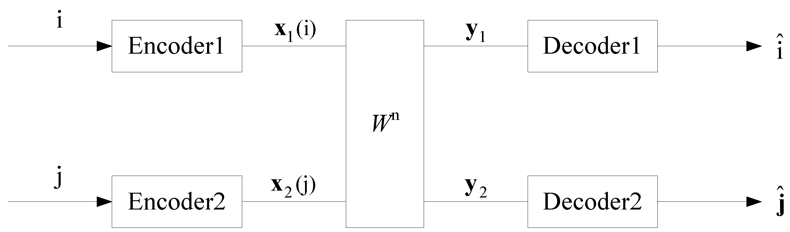
This paper is concerned with a more general IC, which is characterized by a sequence of transition probabilities (see Figure 1). By adopting the information spectrum approach [20,21], we present a general formula for the capacity region of the two-user general IC. From the formula, it can be seen that the capacity region is the union of a family of rectangles, in which each rectangle is determined by a spectral inf-mutual information rate pair. The information spectrum approach, which is based on the limit superior/inferior in probability of a sequence of random variables, has been proved to be powerful in characterizing the limit behavior of a general source/channel. For instance, in [20,22], Han and Verdú proved that the minimum compression rate for a general source equals its spectral sup-entropy rate and the maximum transmission rate for a general point-to-point channel equals its spectral inf-mutual information rate with an optimized input process. Also, the information spectrum approach can be used to derive the capacity region of a general multiple access channel [23]. For more applications of the information spectrum approach, see [21] and the references therein.
The structure of the paper is as follows. In Section 2, the definition of a general IC and the concept of the spectral inf-mutual information rate are introduced. Section 3.1 introduces the general formula for the capacity region proposed in [24]; while, in Section 3.2, a trellis-based algorithm is presented to compute the rate pairs for a stationary memoryless IC with discrete ergodic Markov sources. Section 3.3 presents the numerical results for a GIFC with binary-phase shift-keying (BPSK) modulation. Section 4 provides the detection and decoding algorithms for channels with structured interference. Section 5 concludes this paper.
In this paper, a random variable is denoted by an upper-case letter, say X, while its realization and sample space are denoted by x and , respectively. The sequence of random variables with length n are denoted by , while its realization is denoted by or . We use to denote the probability mass function (pmf) of X if it is discrete or the probability density function (pdf) of X if it is continuous.
2. Basic Definitions and Problem Statement
2.1. General IC
As shown in Figure 1, a general interference channel can be characterized by input alphabets , , output alphabets , and a sequence , in which is a probability transition matrix. That is, for all n,
The marginal distributions of the are given by
Definition 1.
An code for the interference channel consists of the following essentials:
- (a)
- message sets:
- (b)
- sets of codewords:For Sender 1 to transmit message i, Encoder 1 outputs the codeword . Similarly, for Sender 2 to transmit message j, Encoder 2 outputs the codeword .
- (c)
- collections of decoding sets:where for and for . That is, and are the disjoint partitions of and determined in advance, respectively. After receiving , Decoder 1 outputs whenever . Similarly, after receiving , Decoder 2 outputs whenever .
- (d)
- probabilities of decoding errors:where "" denotes the complement of a set. Here we have assumed that each message of and is produced independently with uniform distribution.
Remark 1.
It is optimal to minimize the probability of errors so that the decoding sets and are defined according to the the maximum likelihood decoding [25]. Namely,
and
are selected as the estimates of the transmitted messages by the two receivers, respectively.
Definition 2.
A rate pair is achievable if there exists a sequence of codes such that
Definition 3.
The set of all achievable rates is called the capacity region of the interference channel , which is denoted by .
2.2. Preliminaries of Information-Spectrum Approach
We introduce the notions in [21] as follows.
Definition 4 (liminf in probability).
For a sequence of random variables ,
Definition 5.
If two random variables sequences and satisfy that
for all , and n, they are called independent and denoted by .
Similar to [20], we give
Definition 6.
Let . Given an , for the interference channel , we define the spectral inf-mutual information rate by
where
3. The Capacity Region of General IC
In this section, we firstly present without proof the formula for the capacity region of the general IC derived in [24]. Also the algorithm to compute achievable rate pairs is presented.
3.1. The Main Theorem
Theorem 1.
The capacity region of the interference channel is given by
where is defined as the collection of all satisfying that
3.2. The Algorithm to Compute Achievable Rate Pairs
Theorem 1 provides a general formula for the capacity region of a general IC. However, it is usually difficult to compute the spectral inf-mutual information rates given in (9) and (10). In order to get insights into the interference channels, we make the following assumptions:
- (1)
- the channel is stationary and memoryless, that is, the transition probability of the channel can be written as
- (2)
- sources are restricted to be stationary and ergodic discrete Markov processes.
With the above assumptions, the spectral inf-mutual information rates are reduced as
which can be evaluated by the Monte Carlo method [26,27,28] using BCJR algorithm [29] over a trellis. Actually, any stationary and ergodic discrete Markov source can be depicted by a time-invariant trellis. That is, a trellis section can uniquely specify the source. A trellis section is composed of left (or starting) states and right (or ending) states, which are connected by branches in between. For example, Source can be specified by a trellis as follows.
- Both the left and right states are selected from the set ;
- Each branch is represented by a three-tuple , where is the left state, is the right state, and the symbol is the associated label. We also assume that a branch b is uniquely determined by and ;
- At time , the source starts from state . If at time , the source is in the state , then at time , the source generates a symbol according to the conditional probability and goes into a state such that is a branch. Obviously, when the source runs from time to , a sequence is generated. The Markov property says thatSo the probability of a given sequence with the initial state can be factored as
Similarly, we can represent by a trellis with the state set . Each branch is denoted by , where is the left state, is the right state and the symbol is the associated label. Assume that source starts from the state . If at time , the source is in the state , then at time , the source generates a symbol according to the conditional probability and goes into a state such that is a branch. The probability of a given sequence can be factored as
For simplicity, the initial states have been fixed as and , which can be removed from the equations.
Next we focus on the evaluation of , while can be estimated similarly. Specifically, we can express the limit as
where and can be estimated by similar methods (For continuous , the computations of and can be implemented by substituting pdf for pmf). As an example, we show how to compute . According to the Shannon-McMillan-Breiman theorem [30], it can be seen that, with probability 1,
where stands for . Then evaluating is converted to computing
for a sufficiently long typical sequence . Here, the key is to compute the conditional probabilities for all t. Since both and are hidden Markov sequences, this can be done by performing the BCJR algorithm over the following product trellis.
- The product trellis has the state set , where “×” denotes Cartesian product.
- Each branch is represented by a four-tuple , where is the left state, is the right state. Then and are the associated labels in branch b such that and are branches in and , respectively.
- At time , the sources start from state . If at time , the sources are in the state , then at time , the sources generate symbols according to the conditional probability and go into a state such that is a branch.
The following description shows how to compute by performing the BCJR algorithm. Given the received sequence , we define
- Branch metrics: To each branch , we assign a metricIn the computation of , the metric is replaced by .
- State transition probabilities: The transition probability from to is defined as
- Forward recursion variables: We define the a posteriori probabilitiesThenwhere the values of can be computed recursively by
In summary, the algorithm to estimate the entropy rate is described as follows.
Algorithm 1.
- 1.
- Initializations: Choose a sufficiently large number n. Set the initial state of the trellis to be . The forward recursion variables are initialized as if and otherwise .
- 2.
- Simulations for Sender 1: Generate a Markov sequence according to the trellis of source .
- 3.
- Simulations for Sender 2: Generate a Markov sequence according to the trellis of source .
- 4.
- Simulations for Receiver 1: Generate the received sequence according to the transition probability .
- 5.
- Computations:
Similarly, we can evaluate the entropy rate . Therefore, we obtain the achievable rate .
3.3. Numerical Results
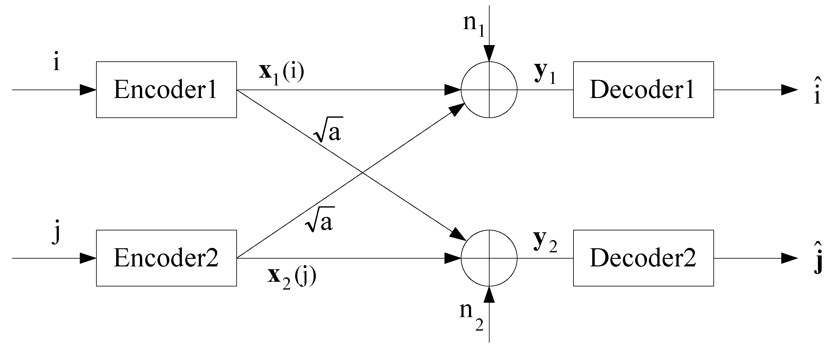
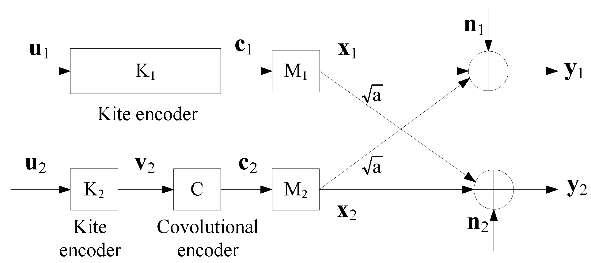
We consider the GIFC as shown in Figure 2, where the channel inputs and are BPSK sequences with power constraints and , respectively; the additive noises and are sequences of independent and identically distributed (i.i.d.) standard Gaussian random variables, which are assumed to be independent of the the channel inputs and ; constant represents the gain of the interference link; the channel outputs and are
We assume that and are the outputs from two (possibly different) generalized trellis encoders driven by independent and uniformly distributed (i.u.d.) input sequences, as proposed in [16]. As examples, we consider two input processes. One is referred to as “UnBPSK”, standing for an i.u.d. BPSK sequence; the other is referred to as “CcBPSK”, standing for an output sequence from the convolutional encoder with the generator matrix driven by an i.u.d. input sequence.
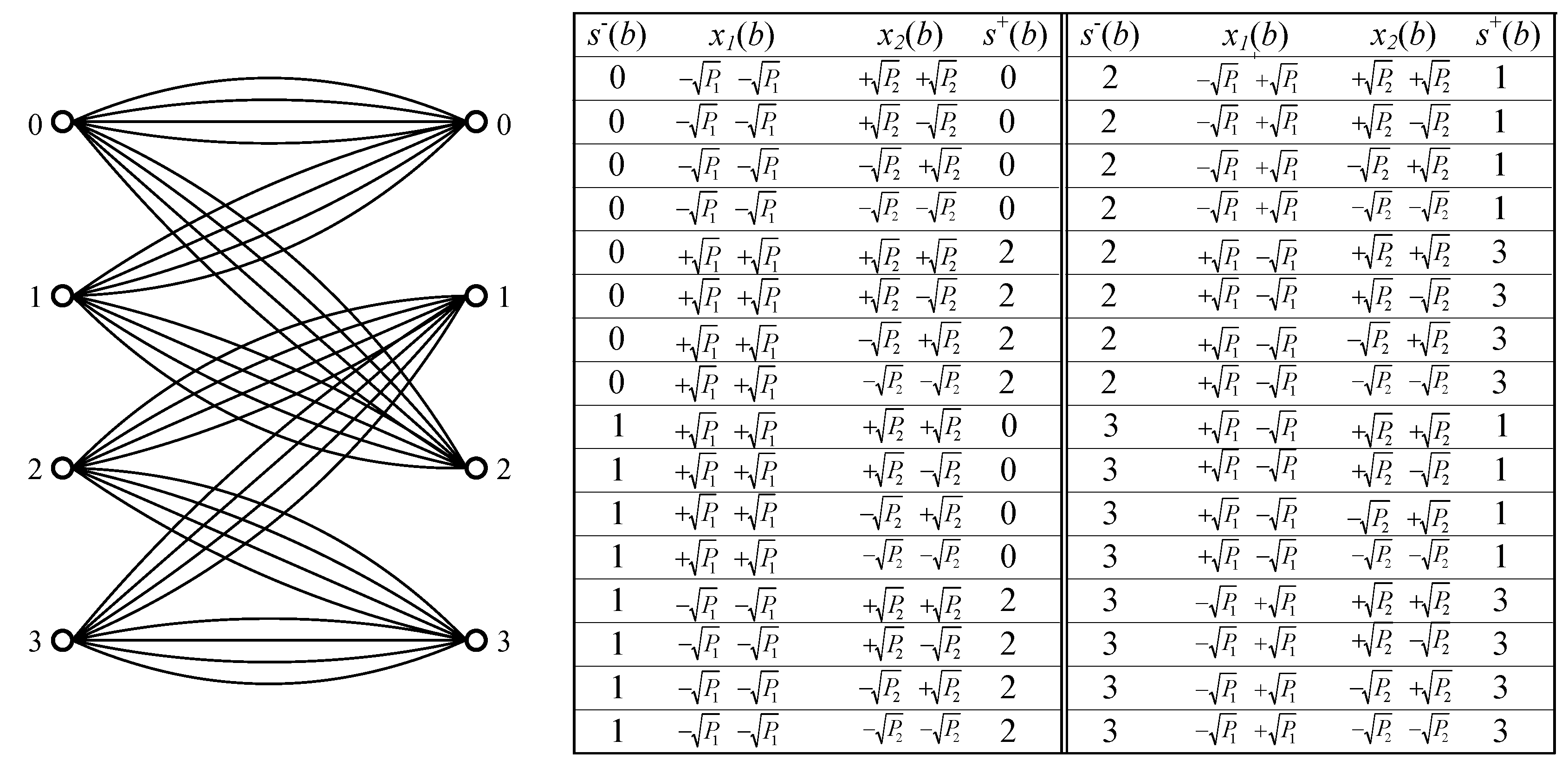
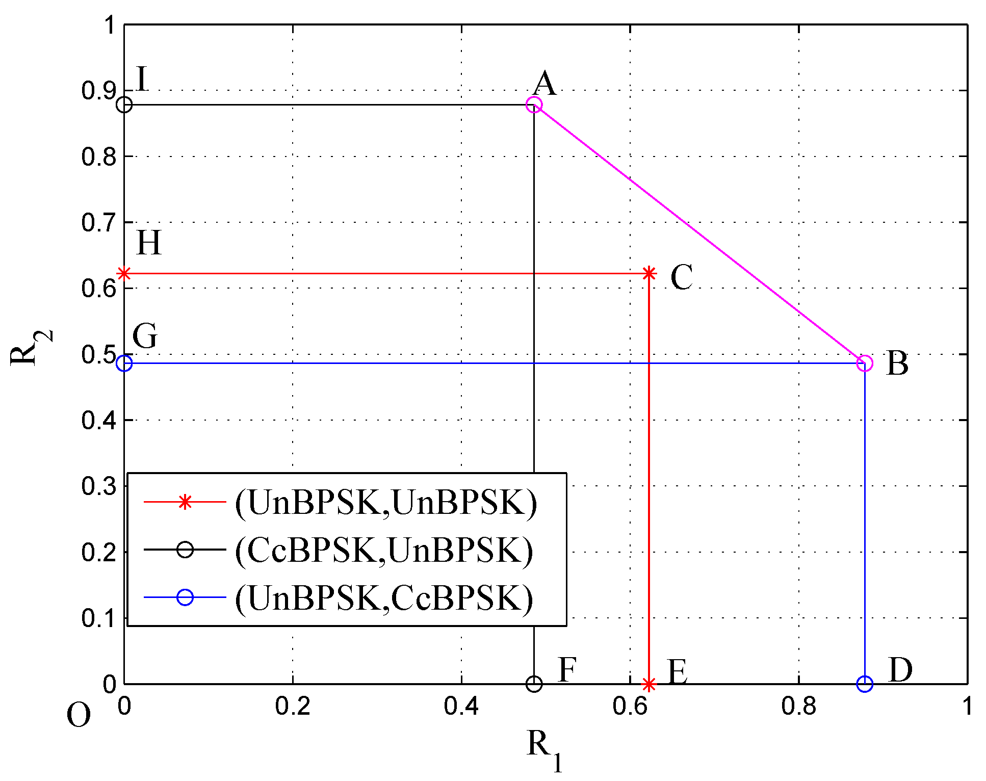
When Sender 1 uses CcBPSK and Sender 2 uses UnBPSK, the trellis representation of the scheme can be seen in Figure 3. The numerical results are presented in Figure 4. There are three rectangles, OECH, ODBG and OFAI, each of which is determined by a pair of spectral inf-mutual information rates. Specifically, the rectangle OECH corresponds to the case when both senders use UnBPSK as inputs; the rectangle ODBG corresponds to the case when Sender 1 uses UnBPSK as input and Sender 2 uses CcBPSK as input; and the rectangle OFAI corresponds to the case when Sender 1 uses CcBPSK as input and Sender 2 uses UnBPSK as input. The point “A” can be achieved by a coding scheme, in which Sender 1 uses a binary linear (coset) code concatenated with the convolutional code and Sender 2 uses a binary linear code, while the point “B” can be achieved similarly. By time-sharing scheme, the points on the line “AB” can be achieved. The point “C” states the limit when the two senders use binary linear codes but take the interference as an i.u.d. additive (BPSK) noise. It is obvious that the area of the pentagonal region ODBAI is greater than that of the rectangle OECH, which hints that the bandwidth-efficiency can be potentially improved by knowing the structure of the interference.
4. Decoding Algorithms for Channels with Structured Interference
The purpose of this section has two-folds. The first is to show the decoding gain achieved by taking into account the structure of the interference. The second is to present a coding scheme to approach the point “B” in Figure 4.
4.1. A Coding Scheme
We design a coding scheme using Kite codes (The main reason that we choose Kite codes is that it is convenient to set up the code rates. Actually, given data length, the code rates of Kite codes can be “continuously” varying from to with satisfactory performance, as shown in [31,32].). Kite codes are a class of low-density parity-check (LDPC) codes, which can be decoded using the sum-product algorithm (SPA) [33,34]. As shown in Figure 5, Sender 1 uses a Kite code (with a parity-check matrix ) and Sender 2 uses a Kite code (with a parity-check matrix ) concatenated with the convolutional code with the generator matrix
Encoding: For Sender 1, a binary sequence of length is encoded by a Kite code into a coded sequence of length N. For Sender 2, a binary sequence of length is firstly encoded by a Kite code into a sequence of length and then the sequence is encoded by the convolutional code with the generator matrix into a coded sequence of length N.
Modulation: The codewords are mapped into the bipolar sequences with (), where is the power. Then we transmit for over the interference channel.
Decoding: After receiving , Receiver 1 tries to recover the transmitted message . Similarly, after receiving , Receiver 2 tries to recover the transmitted message . We will consider several decoding algorithms in the next subsection to recover the transmitted messages.
4.2. Decoding Algorithms
In this subsection, depending on the knowledge about the interference, we design four decoding schemes, including “knowing only the power of the interference”, “knowing the signaling of the interference”, “knowing the CC” and “knowing the whole structure”. We focus on the decoding of Receiver 1, while the decoding of Receiver 2 can be implemented similarly (There is no decoding scheme “Knowing the CC” for User 2 because User 1 has no convolutional structure). All these decoding algorithms will be described as message processing/passing algorithms over normal graphs [35].
4.2.1. Message Processing/Passing Algorithms over Normal Graphs
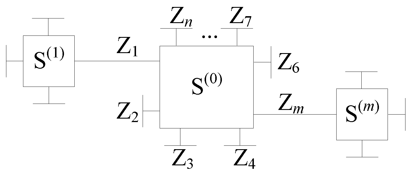
Figure 6 shows a normal graph consisting of edges and vertices, which represent variables and subsystem constraints, respectively. Let be n distinct random variables that form a subsystem . A normal subgraph with edges representing and a vertex representing the constraints can be used to depict the subsystem. Each half-edge (ending with a dongle) may potentially be coupled to some half-edge in other subsystems. For instance, and are displayed to be connected to subsystems and , respectively. We call the corresponding edge full-edge. A message is associated with each edge, which is defined as the pmf/pdf of the corresponding variable. As in [36], we use the notation to denote the message from to . In particular, we use the notation to represent the initial messages “driving” the subsystem . For example, such initial messages can be the a priori probabilities from the source or the a posteriori probabilities computed from the channel observations. Assume that all messages to are available. The vertex , as a message processor, delivers the outgoing message with respect to any given by computing the likelihood function
by considering all the available messages and the system constraints. Since the computation of the likelihood function is irrelevant to the incoming message , we claim that is exactly the so-called extrinsic message.
4.2.2. Knowing Only the Power of the Interference
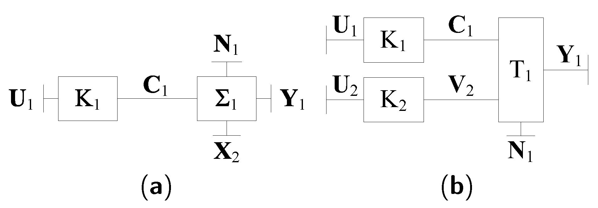
The decoding scheme for “knowing only the power of the interference” is the simplest one, which can be described as a message processing/passing algorithm over the normal graph as shown in Figure 7a. In this scheme, the interference from Sender 2 is treated as a Gaussian distribution with mean zero and variance , where “” is the power and “a” is the square of interference coefficient. That is, Receiver 1 assumes that for . Since for , the decoding algorithm is initialized by the initial messages as follows
for . Then the decoding algorithm uses SPA to compute iteratively the extrinsic messages and . Once these are done, we make the following decisions:
for and . The details about the decoding algorithm are shown as below.
Algorithm 2
(“knowing only the power of the interference”).
- Initialization:
- 1.
- Initialize for and .
- 2.
- Compute for and according to (24).
- 3.
- Set a maximum iteration number J and iteration variable .
- Repeat while :
- End decoding.
4.2.3. Knowing the Signaling of the Interference
The decoding algorithm for this scheme is almost the same as Algorithm 2, see Figure 7a. The difference is that (Bernoulli-1/2 distribution. Strictly speaking, is a shift/scaling version of .) for . So the computation of is changed into
Then the decoding algorithm of “knowing the signaling of the interference” can be shown as below.
Algorithm 3
(“knowing the signaling of the interference”).
- Initialization:
- 1.
- Initialize for and .
- 2.
- Compute for and according to (27).
- 3.
- Set a maximum iteration number J and iteration variable .
- Repeat while :
- End decoding.
4.2.4. Knowing the CC
“Knowing the CC” means that Decoder 1 knows the structure of the convolutional code. This scheme can be described as a message processing/passing algorithm over the normal graph as shown in Figure 7b. Actually, the vertex is a combination of three subsystems, convolutional encoder, modulation and GIFC constraint, which can be specified by a trellis with parallel branches [16]. Therefore, the BCJR algorithm can be used to compute the extrinsic messages for over the trellis . Since the structure of Kite code for Sender 2 is unknown, the constraint of vertex is inactive. In this case, the pmf of variable () is assumed to be Bernoulli-1/2 distribution. There are two strategies to implement the BCJR algorithm. One is called “BCJR-once”, in which the BCJR algorithm is performed only once. The other strategy is called “BCJR-repeat”, in which the BCJR algorithm is performed more than once. In this scheme, the decoding decisions on are modified into
for . These two decoding procedures are described in Algorithms 4 and 5, respectively.
Algorithm 4
(BCJR-once).
- Initialization:
- 1.
- Initialize pmf and for and for .
- 2.
- Compute extrinsic messages for , using BCJR algorithm over the parallel branch trellis .
- 3.
- Set a maximum iteration number J and iteration variable .
- Repeat while :
- End Decoding
Algorithm 5
(BCJR-repeat).
- Initialization:
- 1.
- Initialize pmf and for and for .
- 2.
- Set a maximum iteration number J and iteration variable .
- Repeat while :
- End Decoding
4.2.5. Knowing the Whole Structure
The scheme “knowing the whole structure” for Receiver 1 can also be described as a message processing/passing algorithm over the normal graph shown in Figure 7b. Since knowing the whole structure of the interference, Receiver 1 can decode iteratively utilizing the structure of both users. Using the BCJR algorithm, and are computed simultaneously over the parallel branch trellis . The iterative decoding algorithm is presented in Algorithm 6.
Algorithm 6
(“knowing the whole structure”).
- Initialization:
- 1.
- Initialize pmf and for and for .
- 2.
- Set a maximum iteration number J and iteration variable .
- Repeat while :
- 1.
- Compute extrinsic messages for , and for , using BCJR algorithm over the parallel branch trellis .
- 2.
- Compute extrinsic messages and for and using SPA.
- 3.
- Compute extrinsic messages for using SPA.
- 4.
- 5.
- Compute the syndrome . If , output and and exit the iteration.
- 6.
- Set . If and , report a decoding failure.
- End Decoding
4.3. Numerical Results
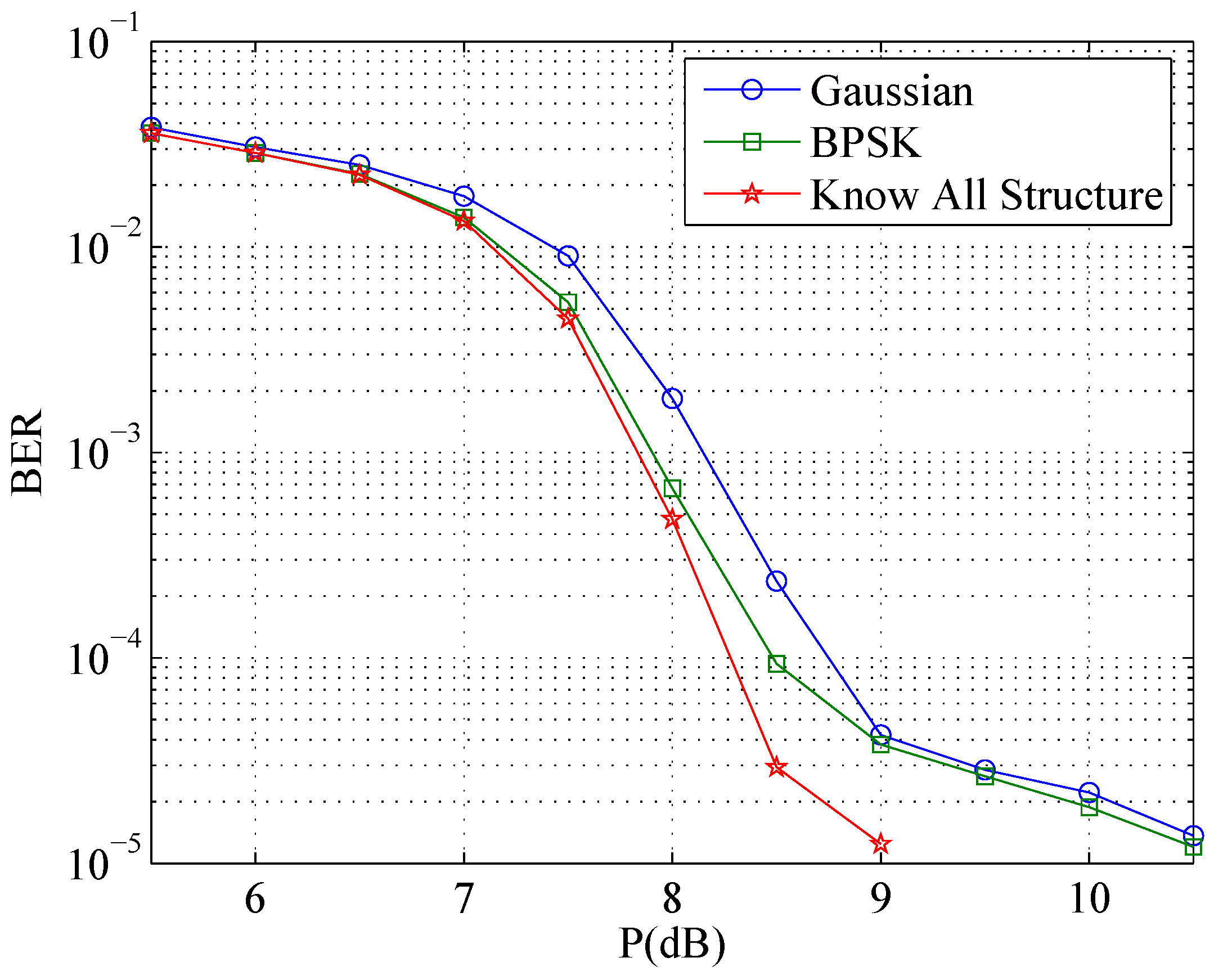
In this subsection, simulation results of the decoding algorithms are shown and analyzed. Simulation parameters of Figure 8 and Figure 9 are presented in Table 1. In these two figures, we let the power constraints of two senders be same, that is, . Here, “Gaussian" stands for the scheme “knowing only the power of the interference”, “BPSK” stands for the scheme “knowing the signaling of the interference”, “BCJR1” stands for the scheme “BCJR-once”, “CONV” stands for the scheme “BCJR-repeat” and “Know All Structure” stands for the scheme “knowing the whole structure”. Figure 8 shows the error performance of Receiver 1. From Figure 8, we can see that, for Receiver 1, more details of the structure of the interference are known, better performance is obtained, that is, the decoding gains get larger. Similarly, Figure 9 gives the error performance of Receiver 2, where the scheme “knowing the whole structure” still has the best performance and the decoding gain can be achieved by taking into account the structure of the interference.
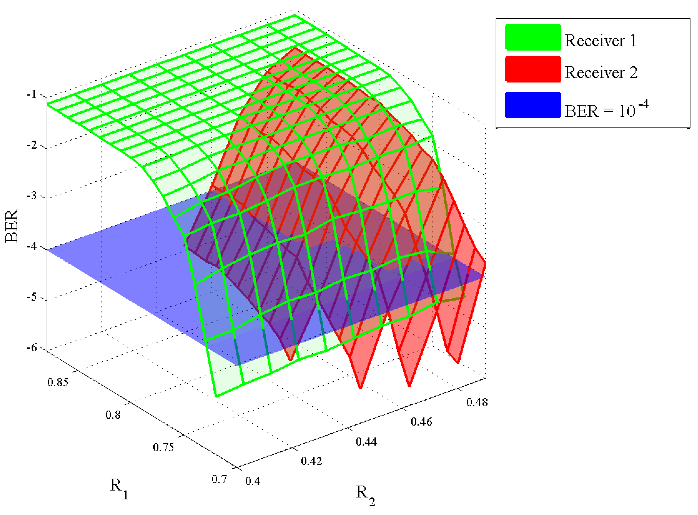
As we said before, another objective in this section is to find out a code rate pair nearest to the point “B” in Figure 4 with bit error rate (BER) performance of . So we do the simulations with different code rate pairs. In the simulations, we adopt the scheme “knowing the whole structure” and gradually decrease the code rates from the point “B” with a step length . Simulation parameters for different code rate pairs are listed in Table 2, while the simulation results are presented using a 3D graph in Figure 10. From the figure, it is obvious that as the code rates of two users are decreasing, the BER also decreases. Finally, we find that the “best” code rate pair is for User 1 and User 2. The theoretical value of the point “B” is about . So we can see that the gap between the result using our decoding scheme and the theoretical value is small.
5. Conclusions
The paper showed that the capacity region of the two-user general IC is the union of a family of rectangles. Each rectangle is defined by a pair of spectral inf-mutual information rates associated with two independent input processes. When the channel is stationary memoryless and the inputs are discrete Markov, we can calculate the defined pair of rates. We can also conclude that taking into account the structure of the interference processes can improve the simplest inner bounds (obtained by treating the interference as noise). Also, a concrete coding scheme to approach the theoretical achievable rate pairs was presented, which showed that the decoding gain can be achieved by considering the structure of the interference.
Acknowledgments
This paper was presented in part at the 2012 IEEE International Symposium Information Theory. This work was partially supported by the China NSFs (Nos. 61601131 and 61401177), the Guangdong NSFs (Nos. 2016A030313727, 2016A030308008 and 2014A030310183) and the Foundation for Distinguished Young Talents in Higher Education of Guangdong (No. 2015KQNCX086). This work was also supported by the Science and Technology Project of Guangzhou (No. 201510010193).
Author Contributions
Xiao Ma conceived the generalized scheme and contributed to the writing of manuscript; Lei Lin provided the proof and completed the paper writing; Chulong Liang performed the experiments and numerical analysis. Xiujie Huang and Baoming Bai helped analyze the data and contributed to the writing of manuscript. All authors have read and approved the final manuscript.
Conflicts of Interest
The authors declare no conflict of interest.
References
- Carleial, A.B. Interference channels. IEEE Trans. Inf. Theory 1978, 24, 60–70. [Google Scholar] [CrossRef]
- Shannon, C.E. Two-way communication channels. In Proceedings of the Fourth Berkeley Symposium on Mathematical Statistics and Probability, Berkely, CA, USA, 20 June–30 July 1960; Neyman, J., Ed.; University of California Press: Berkely, CA, USA, 1961; Volume 1, pp. 611–644. [Google Scholar]
- Ahlswede, R. The capacity region of a channel with two senders and two receivers. Ann. Probab. 1974, 2, 805–814. [Google Scholar] [CrossRef]
- Carleial, A.B. A case where interference does not reduce capacity. IEEE Trans. Inf. Theory 1975, 21, 569–570. [Google Scholar] [CrossRef]
- Han, T.S.; Kobayashi, K. A new achievable rate region for the interference channel. IEEE Trans. Inf. Theory 1981, 27, 49–60. [Google Scholar] [CrossRef]
- El Gamal, A.A.; Costa, M.H.M. The capacity region of a class of deterministic interference channels. IEEE Trans. Inf. Theory 1982, 28, 343–346. [Google Scholar] [CrossRef]
- Costa, M.H.M.; El Gamal, A.A. The capacity region of the discrete memoryless interference channel with strong interference. IEEE Trans. Inf. Theory 1987, 33, 710–711. [Google Scholar] [CrossRef]
- Kramer, G. Outer bounds on the capacity of Gaussian interference channels. IEEE Trans. Inf. Theory 2004, 50, 581–586. [Google Scholar] [CrossRef]
- Sato, H. Two-user communication channels. IEEE Trans. Inf. Theory 1977, 23, 295–304. [Google Scholar] [CrossRef]
- Carleial, A.B. Outer bounds on the capacity of interference channels. IEEE Trans. Inf. Theory 1983, 29, 602–606. [Google Scholar] [CrossRef]
- Sato, H. On degraded Gaussian two-user channels. IEEE Trans. Inf. Theory 1978, 24, 637–640. [Google Scholar] [CrossRef]
- Costa, M.H.M. On the Gaussian interference channel. IEEE Trans. Inf. Theory 1985, 31, 607–615. [Google Scholar] [CrossRef]
- Kramer, G. Review of rate regions for interference channels. In Proceedings of the 2006 IEEE International Zurich Seminar on Communications (IZS), Zurich, Switzerland, 22–24 February 2006; pp. 162–165. [Google Scholar]
- Chong, H.F.; Motani, M.; Garg, H.K.; Gamal, H.E. On the Han-Kobayashi region for the interference channel. IEEE Trans. Inf. Theory 2008, 54, 3188–3195. [Google Scholar] [CrossRef]
- Etkin, R.H.; Tse, D.N.C.; Wang, H. Gaussian interference channel capacity to within one bit. IEEE Trans. Inf. Theory 2008, 54, 5534–5562. [Google Scholar] [CrossRef]
- Huang, X.; Ma, X.; Lin, L.; Bai, B. Accessible Capacity of Secondary Users over the Gaussian Interference Channel. In Proceedings of the IEEE International Symposium on Information Theory, St. Petersburg, Russia, 31 July–5 August 2011; pp. 811–815. [Google Scholar]
- Huang, X.; Ma, X.; Lin, L.; Bai, B. Accessible Capacity of Secondary Users. IEEE Trans. Inf. Theory 2014, 60, 4722–4738. [Google Scholar] [CrossRef]
- Baccelli, F.; El Gamal, A.A.; Tse, D. Interference Networks with Point-to-Point Codes. IEEE Trans. Inf. Theory 2011, 57, 2582–2596. [Google Scholar] [CrossRef]
- Moshksar, K.; Ghasemi, A.; Khandani, A.K. An Alternative To Decoding Interference or Treating Interference As Gaussian Noise. In Proceedings of the IEEE International Symposium on Information Theory, St. Petersburg, Russia, 31 July–5 August 2011; pp. 1176–1180. [Google Scholar]
- Han, T.S.; Verdú, S. Approximation theory of output statistics. IEEE Trans. Inf. Theory 1993, 39, 752–772. [Google Scholar] [CrossRef]
- Han, T.S. Information-Spectrum Methods in Information Theory; Springer: Berlin/Heidelberg, Germany, 2003. [Google Scholar]
- Verdú, S.; Han, T.S. A general formula for channel capacity. IEEE Trans. Inf. Theory 1994, 40, 1147–1157. [Google Scholar] [CrossRef]
- Han, T.S. An information-spectrum approach to capacity theorems for the general multiple-access channel. IEEE Trans. Inf. Theory 1998, 44, 2773–2795. [Google Scholar]
- Lin, L.; Ma, X.; Huang, X.; Bai, B. An information spectrum approach to the capacity region of general interference channel. In Proceedings of the IEEE International Symposium on Information Theory, Cambridge, MA, USA, 1–6 July 2012; pp. 2261–2265. [Google Scholar]
- Etkin, R.H.; Merhav, N.; Ordentlich, E. Error Exponents of Optimum Decoding for the Interference Channel. IEEE Trans. Inf. Theory 2010, 56, 40–56. [Google Scholar] [CrossRef]
- Kavčić, A. On the capacity of Markov sources over noisy channels. In Proceedings of the IEEE 2001 Global Telecommunications Conference, San Antonio, TX, USA, 25–29 November 2001; Volume 5, pp. 2997–3001. [Google Scholar]
- Arnold, D.M.; Loeliger, H.A. On the information rate of binary-input channels with memory. In Proceedings of the IEEE International Conference on Communications, Helsinki, Finland, 11–14 June 2001; Volume 9, pp. 2692–2695. [Google Scholar]
- Pfister, H.D.; Soriaga, J.B.; Siegel, P.H. On the achievable information rates of finite state ISI channels. In Proceedings of the IEEE Global Telecommunications Conference, San Antonio, TX, USA, 25–29 November 2001; Volume 5, pp. 2992–2996. [Google Scholar]
- Bahl, L.R.; Cocke, J.; Jelinek, F.; Raviv, J. Optimal decoding of linear codes for minimizing symbol error rate. IEEE Trans. Inf. Theory 1974, 20, 284–287. [Google Scholar] [CrossRef]
- Cover, T.M.; Thomas, J.A. Elements of Information Theory; John Wiley & Sons: Hoboken, NJ, USA, 1991. [Google Scholar]
- Ma, X.; Zhao, S.; Zhang, K.; Bai, B. Kite codes over Groups. In Proceedings of the IEEE Information Theory Workshop, Paraty, Brazil, 16–20 October 2011; pp. 481–485. [Google Scholar]
- Zhang, K.; Ma, X.; Zhao, S.; Bai, B.; Zhang, X. A New Ensemble of Rate-Compatible LDPC Codes. In Proceedings of the IEEE International Symposium on Information Theory, Cambridge, MA, USA, 1–6 July 2012. [Google Scholar]
- Wiberg, N.; Loeliger, H.A.; Kötter, R. Codes and iterative decoding on general graphs. Eur. Trans. Commun. 1995, 6, 513–526. [Google Scholar]
- Kschischang, F.R.; Frey, B.J.; Loeliger, H.A. Factor graphs and the sum-product algorithm. IEEE Trans. Inf. Theory 2001, 47, 498–519. [Google Scholar] [CrossRef]
- Forney, G.D., Jr. Codes on graphs: Normal realizations. IEEE Trans. Inf. Theory 2001, 47, 520–548. [Google Scholar] [CrossRef]
- Ma, X.; Zhang, K.; Chen, H.; Bai, B. Low Complexity X-EMS Algorithms for Nonbinary LDPC Codes. IEEE Trans. Commun. 2012, 60, 9–13. [Google Scholar] [CrossRef]
Figure 1.
General interference channel .

Figure 2.
Symmetric Gaussian interference channel.

Figure 3.
The trellis section of (CcBPSK, UnBPSK) with 32 branches. For each branch b, and are the left state and the right state, respectively; while the associated symbols and are the transmitted signals at Sender 1 and Sender 2, respectively.
Figure 3.
The trellis section of (CcBPSK, UnBPSK) with 32 branches. For each branch b, and are the left state and the right state, respectively; while the associated symbols and are the transmitted signals at Sender 1 and Sender 2, respectively.

Figure 4.
The evaluated achievable rate pairs of a specific Gaussian interference channel (GIFC), where and . The rectangle OECH with legend “(UnBPSK, UnBPSK)” corresponds to the case when both senders use UnBPSK as inputs; the rectangle ODBG with legend “(UnBPSK, CcBPSK)” corresponds to the case when Sender 1 uses UnBPSK as input and Sender 2 uses CcBPSK as input; and the rectangle OFAI with legend “(CcBPSK, UnBPSK)” corresponds to the case when Sender 1 uses CcBPSK as input and Sender 2 uses UnBPSK as input.

Figure 5.
A coding scheme for the two-user GIFC.

Figure 6.
A normal graph of a general (sub)system.

Figure 7.
The normal graphs: (a) stands for the normal graph of “knowing only the power of the interference” and “knowing the signaling of the interference” for Decoder 1; (b) stands for the normal graph of “knowing the CC” and “knowing the whole structure” for Decoder 1.
Figure 7.
The normal graphs: (a) stands for the normal graph of “knowing only the power of the interference” and “knowing the signaling of the interference” for Decoder 1; (b) stands for the normal graph of “knowing the CC” and “knowing the whole structure” for Decoder 1.

Figure 8.
The error performance of Receiver 1. “Gaussian” stands for the scheme “knowing only the power of the interference”, “BPSK” stands for the scheme “knowing the signaling of the interference”, “BCJR1” stands for the scheme “BCJR-once”, “CONV” stands for the scheme “BCJR-repeat” and “Know All Structure” stands for the scheme “knowing the whole structure”.

Figure 9.
The error performance of Receiver 2. “Gaussian” stands for the scheme “knowing only the power of the interference”, “BPSK” stands for the scheme “knowing the signaling of the interference” and “Know All Structure” stands for the scheme “knowing the whole structure”.
Figure 9.
The error performance of Receiver 2. “Gaussian” stands for the scheme “knowing only the power of the interference”, “BPSK” stands for the scheme “knowing the signaling of the interference” and “Know All Structure” stands for the scheme “knowing the whole structure”.

Figure 10.
Error performance of two users with different code rate pairs . Blue plane represents BER level, green surface stands for the error performance of Receiver 1 and red surface stands for the error performance of Receiver 2.
Figure 10.
Error performance of two users with different code rate pairs . Blue plane represents BER level, green surface stands for the error performance of Receiver 1 and red surface stands for the error performance of Receiver 2.


Table 1.
Parameters of the bit error rate (BER) performance simulations.
| Parameters | Values |
|---|---|
| Square of interference coefficient a | 0.5 |
| Maximum iteration number J | 200 |
| Kite Code of Sender 1 | |
| Kite Code of Sender 2 | |
| Generator matrix | |
| Code rate pair |
Table 2.
Parameters of the simulations for different code rate pairs.
| Parameters | Values |
|---|---|
| Square of interference coefficient a | |
| Maximum iteration number J | 200 |
| Code length N of Kite Code of Sender 1 | 10000 |
| Code length of Kite Code of Sender 2 | 5000 |
| Generator matrix | |
| Step length | 100 |
| Range of message length | |
| Range of message length |
© 2017 by the authors. Licensee MDPI, Basel, Switzerland. This article is an open access article distributed under the terms and conditions of the Creative Commons Attribution (CC BY) license (http://creativecommons.org/licenses/by/4.0/).
Share and Cite
MDPI and ACS Style
Lin, L.; Ma, X.; Liang, C.; Huang, X.; Bai, B. An Information-Spectrum Approach to the Capacity Region of the Interference Channel. Entropy 2017, 19, 270. https://doi.org/10.3390/e19060270
AMA Style
Lin L, Ma X, Liang C, Huang X, Bai B. An Information-Spectrum Approach to the Capacity Region of the Interference Channel. Entropy. 2017; 19(6):270. https://doi.org/10.3390/e19060270
Chicago/Turabian StyleLin, Lei, Xiao Ma, Chulong Liang, Xiujie Huang, and Baoming Bai. 2017. "An Information-Spectrum Approach to the Capacity Region of the Interference Channel" Entropy 19, no. 6: 270. https://doi.org/10.3390/e19060270
Note that from the first issue of 2016, this journal uses article numbers instead of page numbers. See further details here.