Morphological and Genetic Diversity of Sea Buckthorn (Hippophae rhamnoides L.) in the Karakoram Mountains of Northern Pakistan

Abstract

Sea buckthorn (Hippophae rhamnoides L.) is a dioecious, wind-pollinated shrub growing in Eurasia including the Karakoram Mountains of Pakistan (Gilgit-Baltistan territory). Contrary to the situation in other countries, in Pakistan this species is heavily underutilized. Moreover, a striking diversity of berry colors and shapes in Pakistan raises the question: which varieties might be more suitable for different national and international markets? Therefore, both morphological and genetic diversity of sea buckthorn were studied to characterize and evaluate the present variability, including hypothetically ongoing domestication processes. Overall, 300 sea buckthorn individuals were sampled from eight different populations and classified as wild and supposedly domesticated stands. Dendrometric, fruit and leaf morphometric traits were recorded. Twelve EST-SSRs (expressed sequence tags-simple sequence repeats) markers were used for genotyping. Significant differences in morphological traits were found across populations and between wild and village stands. A significant correlation was found between leaf area and altitude. Twenty-two color shades of berries and 20 dorsal and 15 ventral color shades of leaves were distinguished. Mean genetic diversity was comparatively high (H_e = 0.699). In total, three distinct genetic clusters were observed that corresponded to the populations’ geographic locations. Considering high allelic richness and genetic diversity, the Gilgit-Baltistan territory seems to be a promising source for selection of improved germplasm in sea buckthorn.

1. Introduction

Sea buckthorn (Hippophae rhamnoides L.; 2n = 24; family Elaeagnaceae) is a shrubby species of native Eurasian plant communities ranging within 27°–69° N latitude (from Russia to Pakistan) and 7° W–122° E longitude (from Spain to Mongolia) with a center of origin on the Qinghai–Tibet Plateau. It is a dioecious, wind-pollinated, 1–9 m tall shrub or tree capable of propagating clonally. As a pioneer species it spreads on marginal soils across a vast range of dry temperate and cold desert soils [1,2] and requires minimum annual rainfall of 250 mm for proper growth. Sea buckthorn possesses a specialized root system that can fix N₂ through forming Frankia-actinorhizal root nodules [3] and is known to improve the soil structure, which makes it an ideal species for land reclamation and wildlife habitat improvement [4].

The flowering of male and female plants takes place between mid of April and May before the leaves appear. It requires 2–3 days for dehiscence of pollen grains, which are viable up to 10 days after anthesis, and formation of pollen tubes happens about 72 h after pollination [5,6]. The stigma remains most receptive for three days post-anthesis. The number of fruits produced during the season depends on the growing conditions of the previous year when flower buds are formed [7]. Sea buckthorn requires 3–4 years to start fruiting depending upon the propagation method (seed or cuttings) and produces yellow, orange or red berries (6–9 mm in diameter) containing a single seed [8]. Berry color seems to be correlated with the amount of tannins (proanthocyanins) [9].

The global sea buckthorn production area is unknown and country-wise data lack a standardized assessment: China’s natural production range covers more than 10,000 km² [10], Mongolia’s natural range is 29,000 km² (data only available for Uvs province) [11], former USSR covers 472 km² [12], while in India the production areas of naturally grown sea buckthorn are available only for Leh (115 km²) [13] and Uttarakhand (38 km²) [14]. There is a high potential of different kinds of products from sea buckthorn berries including cosmetics (mainly in Russia and China) and food (mainly in Europe). According to an assessment of the sea buckthorn business in Europe, Russia, New Independent States countries and China in the year 2005, the value of by-products from berries and leaves accounts approximately for 42 million Euros [15]. Pakistan includes many thousands of hectares of sea buckthorn growing naturally in the Gilgit and Baltistan regions, of which only about 20% are utilized [8] to produce a variety of products. Hence, the species has a great untapped economic and social potential with important plant genetic resources whose use may add to rural livelihoods.

The species has several unique medicinal properties, such as high concentrations of vitamins, tannins, triterpenoids, phospholipids, caumarin, catechins, leucoenthocyans, flavanols, alkaloids, serotonin, and unsaturated fatty acids [16,17,18] providing supplements for a healthy food and a variety of ingredients for medical use [19] against obesity, diabetes, cardiovascular disease, cancer, ulcer, inflammation, immune system disease, burn wounds, and radiation damage [20,21].

Wild sea buckthorn germplasm, however, varies widely with respect to morphometrical, visual, nutritional, and genetic properties [8,22,23], which has implications for the quality of products. This variation, especially for leaf and fruit morphometry and color is likely controlled by a combination of factors rather than by a single factor. First, the wide distribution of sea buckthorn throughout Asia, including the Gilgit and Baltistan regions implies the species’ occurrence in many climatic zones [12,24]. Second, altitudinal [25] and environmental stresses such as water availability [26,27] and soil nutrient status [28] affect sea buckthorn traits and sexual propagation [18]. Third, geographical physical barriers (mountain ranges, glaciers, rivers, etc.) may cause genetic differentiation by preventing gene flow potentially resulting in allopatric divergence as it was observed for sea buckthorn in the Himalayan Mountains [29,30] and for other species [31,32]. Fourth, the genetic setup itself may play a role in phenotypic variation, although to our knowledge no study has so far analyzed this association in sea buckthorn. Fifth, human-induced plant material exchange, overexploitation, and domestication could have negative consequences on population structures leading to genetic bottleneck effects [33,34,35]. For northern Pakistan, the identification and characterization of superior ecotypes and populations with respect to yield, nutritional characteristics, time of ripening, and genetic constitution are important to allow for the collection of berries of higher nutritional quality and other market demanded properties, such as fruit size and color.

There are several genetic studies of sea buckthorn based on RAPD (random-amplified polymorphic DNA) [36,37,38,39,40,41], AFLP (amplified fragment length polymorphism) [42,43], SSR (simple sequence repeat, microsatellite) [44], ISSR (inter simple sequence repeat) [25,45] and gene-based EST-SSR (expressed sequence tags-simple sequence repeat) [46,47] markers. The EST-SSR markers are more likely to reflect adaptive genetic variation than other markers since they are linked with expressed (functional) genes and usually found in 3′ untranslated regions (3′-UTRs) of expressed sequence tag (EST) sequences.

Therefore, this study aims at estimating the morphological and genetic variability by measuring morphological traits and genotyping EST-SSR markers, respectively. The specific objectives of the study were to (1) compare the dendrometry, fruit traits and genetic diversity patterns of sea buckthorn among different populations, (2) analyze the influence of domestication processes on genetic and morphological traits by comparing wild and supposedly domesticated village stands, and (3) evaluate the genetic variation and differentiation found in the study area.

2. Materials and Methods

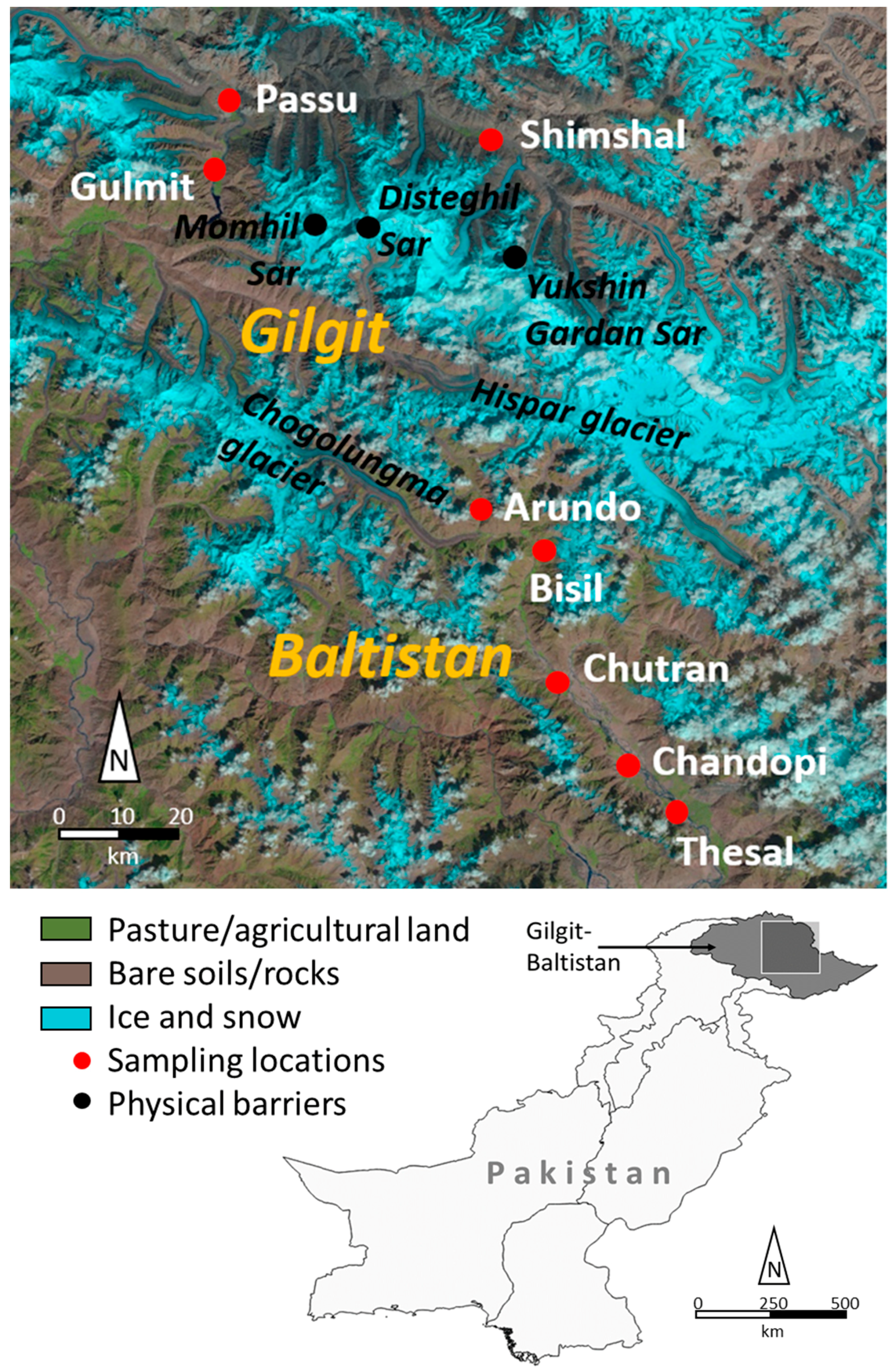
2.1. Plant Material and Sampling Area

The field study was carried out in September–November 2016 in the Karakoram Mountains of northern Pakistan. To quantify the morphological and molecular diversity, eight populations at different altitudes in two regions, Gilgit (Shimshal, Passu, Gulmit) and Baltistan (Thesal, Chandopi, Chutran, Bisil and Arando) (Figure 1), were selected, and 300 individual plants were sampled in total (

Table 1. Average geographic coordinates of the eight sea buckthorn populations studied in the Gilgit and Baltistan regions, Pakistan.

Region	Population	No. of Individuals	Longitude E	Latitude N	Elevation, m.a.s.l.
Gilgit	Gulmit	60	36.4049805	74.8734	2525
	Passu	40	36.4558832	74.8997	2516
	Shimshal	60	36.4412537	75.3008	3112
Baltistan	Thesal	20	35.4697578	75.6654	2275
	Chandopi	40	35.5428859	75.5711	2330
	Chutran	40	35.7268528	75.4046	2435
	Bisil	20	35.8568179	75.4156	2655
	Arando	20	35.8695884	75.3677	2700
Total		300

). To test for the effects of human selection on sea buckthorn, populations were subdivided into “village” (within the residential area) and “wild” stands (a minimum distance of 1 km from the nearest house), forming corresponding stand pairs. Per stand, ten individuals were randomly sampled based on a nearest neighbor criterion with a minimum distance of 100 m between individuals to avoid sampling of clonal plants [48]. Depending on the size of villages, occasionally more than one stand pair was sampled, resulting in more than 20 individuals per population. The exact location and altitude (meter above sea level, m.a.s.l.) of all individuals were determined with a hand-held GPS device (Garmin-eTrex 30, horizontal accuracy ± 2 m, GARMIN^® Ltd., Southampton, UK).

2.2. Dendrometric Traits

Height (cm) of shrubs was measured with the help of a measuring pole, whereby the height of the tree was determined by intercept theorems [49]. The stem girth (cm) at the shrub or tree base was determined twice (perpendicular axes) with a digital Vernier caliper. Subsequently, the geometric mean was transformed to the diameter. Plant canopy area (m²) was calculated from the canopy diameters measured in the N-S and W-E directions.

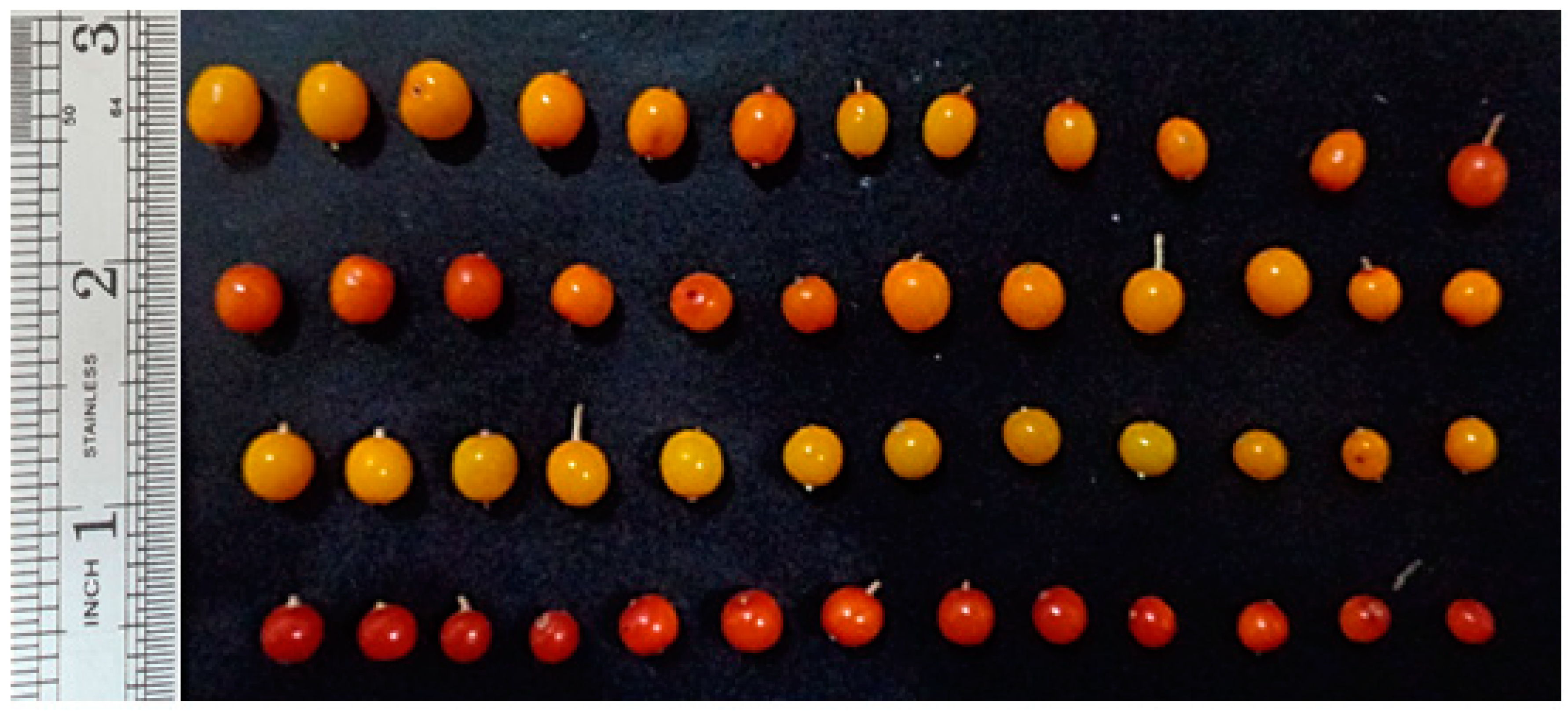
2.3. Leaf and Fruit Morphometry Traits

Ten leaves per individual were randomly collected for length measurements including the petiole and width (both in mm) at the widest point with a digital Vernier caliper. Leaf area (mm²) was calculated by assuming an oval-oblong shape of a leaf. To assess differences in leaf shape, the length to width ratio was calculated. Afterward, leaves were stored and air dried in filter bags for further genetic analysis (see below).

For each individual, around 20 grams of berries (Figure 2) were collected randomly. A digital balance (accuracy: ±0.01 g, Tomopol p250) was used to measure the bulked weight (g) of 20 berries. Out of this, 10 randomly chosen berries were measured with the Vernier caliper to determine length and width (both in mm) at the widest point of each fruit. Fruit volume (mm³) was calculated by assuming an ellipsoid shape of the berry. As for the leaves, fruit length to width ratio was calculated. Afterwards, fruits were air dried in the shade until a constant weight was obtained. Based on weight differences moisture contents were calculated.

Means and coefficient of variation (CV) were calculated for all morphometric traits to identify highly variable and therefore promising parameters for harvesting and possible breeding of sea buckthorn.

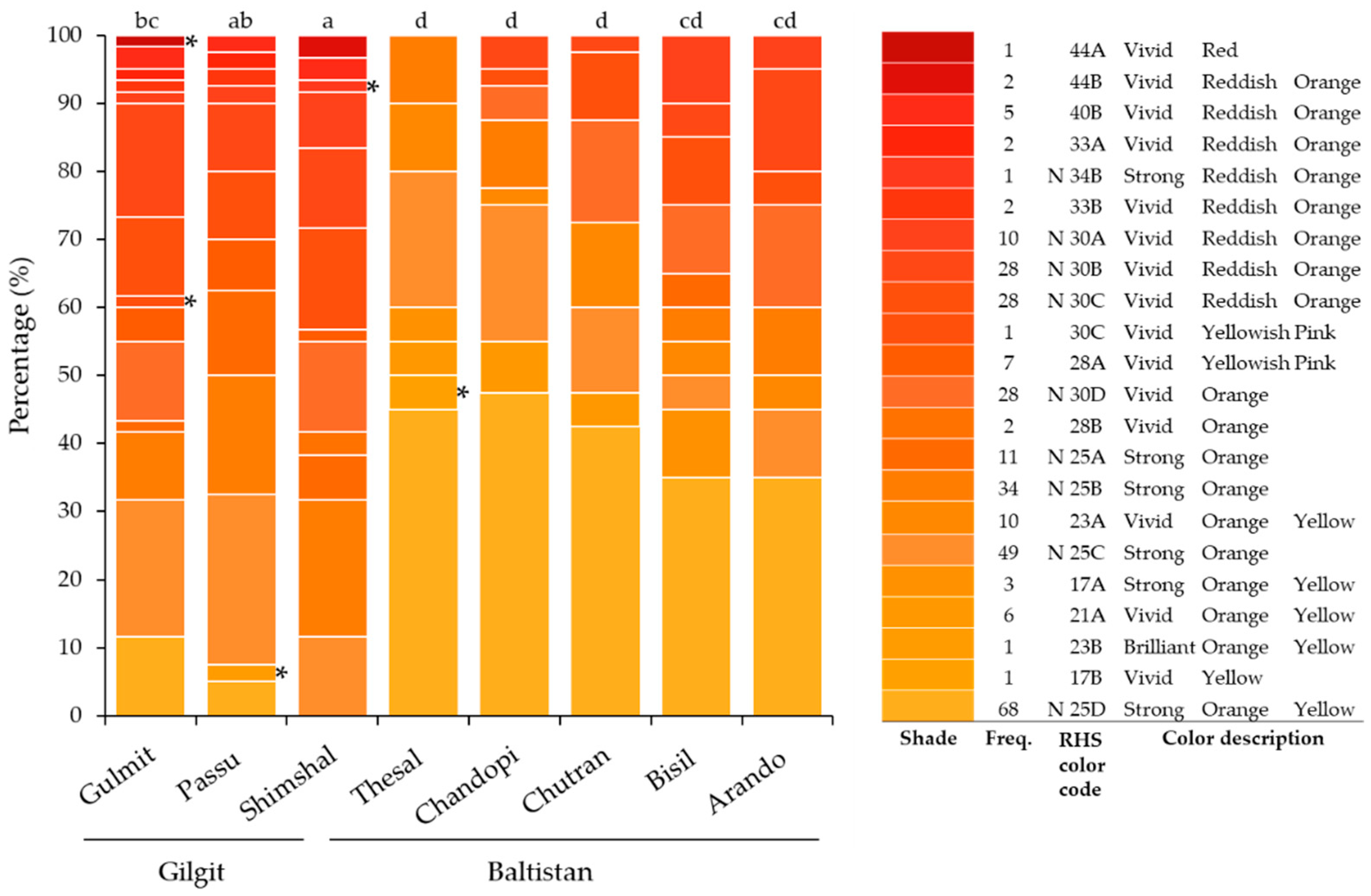
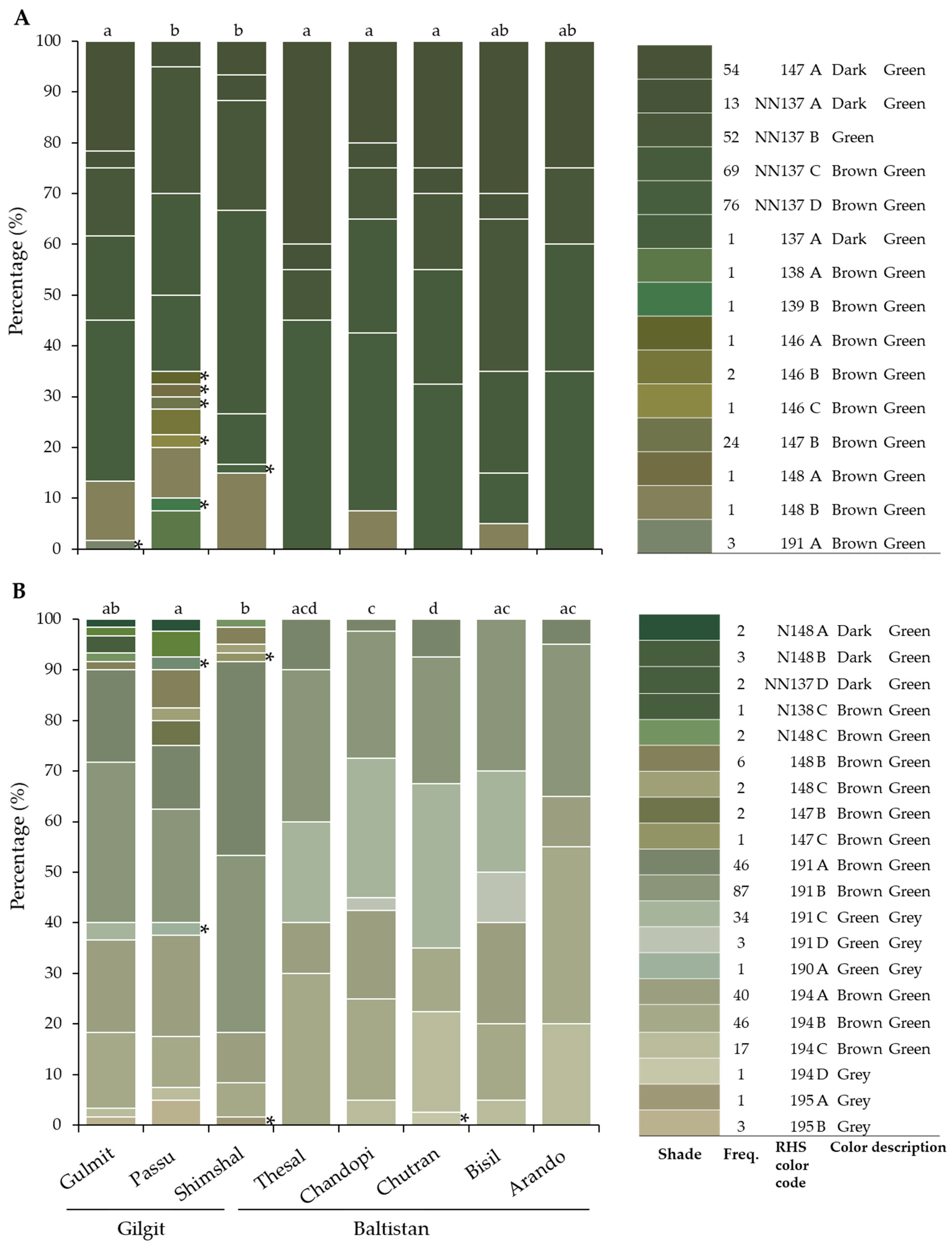
2.4. Leaf and Fruit Colors

The color of leaves (dorsal and ventral part) and berries was determined using the Royal Horticultural Society (RHS) color charts (sixth edition, 2015, RHS media, 80 Vincent-Square, London, UK). The 920 RHS coded reference colors are a standard to identify plant tissue colors used by horticulturalists worldwide. The RHS color code was decoded into the Red-Green-Blue (RGB) colors available at the RHS webpage (http://rhscf.orgfree.com, accessed on 2 February 2017) and used for visual presentation (Figure 3 and Figure 4).

2.5. DNA Isolation and EST-SSR Analysis

Total genomic DNA was extracted from each of the 300 leaf samples using the DNeasy™ 96 Plant Kit (Qiagen GmbH, Hilden, Germany). Twelve already established and highly polymorphic EST-based SSR markers–six USMM (1, 3, 7, 16, 24, and 25, respectively; [46]) and six HrMS (003, 004, 010, 012, 014, and 018; respectively, [47]) markers were screened and used in this study. Forward primers of these markers were labeled with fluorescent dyes to design four different multiplexes depending upon the PCR (polymerase chain reaction) product sizes. The PCR amplifications were performed in a total volume of 15 μL containing 2 μL of genomic DNA (about 10 ng), 1X reaction buffer (0.8 M Tris-HCl pH 9.0, 0.2 M (NH₄)₂SO₄, 0.2% w/v Tween-20; Solis BioDyne, Tartu, Estonia), 2.5 mM MgCl₂, 0.2 mM of each dNTP, 0.3 μM of each forward and reverse primer and 1 unit of Taq DNA polymerase (HOT FIREPol^® DNA Polymerase, Solis BioDyne, Tartu, Estonia). The amplification protocol was as follows: an initial denaturation step at 95 °C for 15 min, followed by 30 cycles consisting of a denaturing step at 94 °C for 1 min, an annealing step at 55 °C for 30 s and an extension step at 72 °C for 1 min. After 30 cycles, a final extension step at 72 °C for 20 min was included. Reproducibility was checked by repeating positive and negative controls in all reaction plates. The PCR fragments were separated and sized on an ABI 3130xl Genetic Analyzer (Applied Biosystems Inc., Foster City, CA, USA). The GS 500 ROX (Applied Biosystems Inc.) was used as an internal size standard. The genotyping was done using the GeneMapper 4.1^® software (Applied Biosystems Inc.).

2.6. Data Analysis

All metric morphological data were analyzed with the R-software (version 3.3.3, R core team, 2017, Vienna, Austria) using the multcomp package [50]. Data were checked for normal distribution of residuals and homogeneity of variances followed by t-tests or analyses of variance (ANOVA). The Tukey-Kramer post hoc test was used to identify significant differences among subgroups, which is considered to be the most suitable test for unbalanced designs according to Herberich et al. [51]. The total mean of populations and stands (village and wild) was calculated to indicate local variation. For color variation (nominal data) of leaves and fruits, Fisher’s exact Chi (χ²)-square test and post hoc tests (pairwise nominal independence) were performed using the “rcompanion” package in R [52]. Additionally, Pearson correlations were performed to estimate the significance of the correlation between altitude and leaf area, and between altitude and fruit color shade.

MICRO-CHECKER [53] was used to test and correct for potential genotyping errors due to stuttering, large-allele dropout, and null-alleles. Genetic variation parameters such as the number of alleles per locus (N_a), the number of private alleles, allelic richness, percentage of polymorphic loci, expected (H_e) and observed (H_o) heterozygosities were determined for each population. In addition, deviations from the Hardy-Weinberg equilibrium (HWE) were checked by χ²-tests for each locus per population. All parameters were calculated using the GenAlEx 6.5 software [54] except for allelic richness which was calculated to account for differences in sample size with the HP-Rare program 1.0 [55] considering a sample size of 40 individuals in each sample.

Isolation-by-distance (IBD) was tested with a Mantel test using pairwise geographic distance and standardized genetic differentiation G’_ST [56] with 1000 random permutations in GenAlEx 6.5. To analyze differentiation between populations and characterize population genetic structure, an analysis of molecular variance (AMOVA) was applied with 999 permutations. F-statistics (F_ST, F_IS, and F_IT; range: 0–1; null hypothesis: indices equal to zero) were calculated using the same software. F_ST indicates the extent of population differentiation. F_IS and F_IT are indices of fixation of an individual relative to its population and the total sample, respectively. Their positive values are indication of deficiency of the observed heterozygosity relative to the expected one, which could be a signature of inbreeding, population subdivision (Wahlund effect) or mis-genotyping heterozygotes as homozygotes due to null-alleles or large-allele dropout. In addition, Genepop 4.7 software was employed to calculate population-wise fixation indices (F_IS) and their significance with 10,000 dememorizations, 100 batches and 5000 iterations per batch for the Markov chain parameters. The genetic clusters (K) were inferred using EST-SSRs and the Bayesian approach implemented in the STRUCTURE 2.3.4 software [57]. The admixture model with correlated allele frequencies and a burn-in period of 100,000 Markov Chain Monte Carlo (MCMC) replicates were used. We tested from 1 to 12 possible clusters (K), using 10 iterations per each of them. The most likely number of K was determined according to the ΔK method implemented in the open-access software STRUCTURE-HARVESTER [58], considering K with the highest value of ΔK and the lowest value of mean posterior probability of the data (LnP(D)) [59]. Microsoft excel was used for summation and graphical representation of the results obtained by STRUCTURE 2.3.4.

3. Results

3.1. Dendrometric Traits

Average plant height ranged from 138 to 198 cm with an individual minimum and maximum of 10 and 450 cm, respectively (

Table 2. Average morphological traits of sea buckthorn at the eight populations and their corresponding stands studied in the Gilgit and Baltistan regions, Pakistan.

Grouping	Population/Stand		Dendrometry						Leaf				Fruit
			Height, cm		Stem Diameter, cm		Canopy, m2		Area, mm2		Length to Width Ratio		Volume, mm3		Length to Width Ratio		20-berry wt., g		Moisture, %
Populations	Gulmit		146	b	5.1	ab	2.4	ab	85	a	7.5	b	75	a	1.1	b	1.6	a	66	a
	Passu		138	ab	4.4	a	1.5	a	93	a	7.2	ab	85	a	1.1	b	1.8	a	66	ab
	Shimshal		174	c	4.9	b	2.1	ab	192	e	6.5	a	150	c	1.1	a	3.1	b	77	c
	Thesal		193	ac	4.5	ab	3.1	bc	98	ab	7.9	bc	123	bc	1.2	b	2.5	b	67	ab
	Chandopi		198	bc	6.0	ab	3.5	c	131	bc	7.8	bc	135	bc	1.2	b	2.9	b	67	ab
	Chutran		156	b	4.6	ab	2.6	bc	129	bc	7.9	bc	120	b	1.2	b	2.6	b	69	ab
	Bisil		189	bc	4.1	ab	2.5	ac	186	de	8.8	c	129	bc	1.1	ab	2.9	b	70	ab
	Arando		151	bc	3.7	ab	2.6	ac	155	cd	8.6	c	141	bc	1.2	b	2.9	b	71	b
	p-value		<0.001		<0.001		<0.001		<0.001		<0.001		<0.001		<0.001		<0.001		<0.001
Stands	Wild		160		4.8		2.5		126	a	7.7		117		1.1		2.5		70
	Village		177		5.7		2.5		141	b	7.8		122		1.1		2.6		69
	p-value		0.050		0.140		0.950		0.009		0.527		0.257		0.817		0.780		0.130
Populations*stands	Gulmit	Wild	162	ab	6.2	ab	2.5	ac	84	a	7.3	ace	75	a	1.1	ac	1.7	a	68	ac
		Village	131	a	3.9	a	2.3	ac	85	a	7.6	bcd	74	a	1.1	ac	1.5	a	64	a
	Passu	Wild	125	a	3.6	a	1.3	a	80	a	6.8	ac	91	ab	1.1	ac	1.9	ac	67	ac
		Village	151	ad	5.2	ab	1.6	ab	106	ab	7.6	ad	80	a	1.2	ac	1.7	ab	66	ab
	Shimshal	Wild	128	a	3.6	a	1.6	ab	171	ef	6.4	a	153	e	1.2	ab	3.2	e	82	d
		Village	221	b	6.2	b	2.5	ac	213	g	6.6	ab	148	ce	1.1	a	2.9	de	72	c
	Thesal	Wild	155	ab	4.3	a	2.5	ac	92	ab	7.7	ad	104	acd	1.2	ac	2.3	ade	66	ac
		Village	231	bd	4.7	a	3.5	bc	105	ac	8.1	ad	141	de	1.2	ac	2.7	bce	68	ac
	Chandopi	Wild	210	bcd	7.5	ab	4.2	c	143	bcdf	8.3	cd	147	de	1.1	ac	3.2	e	70	bc
		Village	185	ab	4.5	a	2.9	ac	120	abd	7.3	ad	124	bde	1.2	c	2.6	ce	64	ab
	Chutran	Wild	174	ab	6.1	ab	2.9	ac	124	abd	7.6	ad	109	ad	1.1	ac	2.3	acd	65	ab
		Village	138	ac	3.1	a	2.3	ab	134	bce	8.1	cd	131	de	1.1	ac	2.8	de	73	c
	Bisil	Wild	187	ab	4.1	a	2.5	ac	173	deg	8.6	cd	117	ade	1.1	ac	2.7	bce	69	ac
		Village	192	ab	4.0	a	2.5	ac	199	fg	9.1	d	141	de	1.1	ac	3.1	de	71	ac
	Arando	Wild	137	ab	3.4	a	2.5	ac	145	bcdf	8.9	de	142	de	1.2	bc	3.1	ce	71	ac
		Village	165	ab	3.9	a	2.6	ac	166	cdeg	8.2	bcd	139	de	1.1	ac	2.8	bce	71	ac
	p-value		<0.001		<0.001		0.030		0.028		0.095		0.021		0.173		0.042		<0.001
Grand mean			165		5.3		2.5		132		7.5		117		1.1		2.5		69
CV, %			45		62		70		46		20		39		12		41		11

Letters indicate the significance of similarities among sites (populations sharing the same letters are similar and vice versa). CV—coefficient of variation.

). Average stem diameter ranged from 3.7 to 6.0 cm with an individual minimum and maximum of 0.8 and 82.0 cm, respectively (Table 2). Canopy area averaged 2.5 m² ranging from 0.1 to 15.0 m² and had the highest CV (70%, Table 2). As a general tendency, plants in village stands were higher than plants in wild stands. This difference was the most pronounced and statistically significant in Thesal followed by Shimshal, Bisil, Arando, and Passu.

3.2. Leaf and Fruit Morphometry Traits

Significant variation was found in the leaf traits between village and wild stands, for population*stand interactions and among populations (Table 2). Leaf area (mm²) was higher in village stands than in wild stands except for Chandopi, whereas mean values of populations (village and wild stands together) were the highest in Shimshal followed by Bisil, Arando, Chandopi, Chutran, Thesal, Passu and Gulmit (Table 2). A significant positive correlation (r = 0.493, p = < 0.001) was found between leaf area and altitude. The leaf length to width ratio indicates the narrowness or wideness of the leaf; the widest leaves were found in Bisil (8.8 cm) and the narrowest in Shimshal (6.5 cm; Table 2).

Significant variation was also found in all fruit traits within population*stands and among populations, but not between wild and village stands (Table 2). Fruit volume was highest in Shimshal (150 mm³) and lowest in Gulmit (75 mm³) (Table 2). The maximum and minimum weight of 20 berries was 6.28 and 1.08 g, respectively. Means of 20-berry-weight were lowest in Passu and Gulmit, whereas they were highest in Shimshal. This trend was also reflected in moisture content, which was the highest in Shimshal (77%) and lowest in Passu and Gulmit (66% each). All leaf and fruit morphometric parameters showed the same trend of having significantly lower values in Passu and Gulmit as compared to the other populations. The CV was the highest for leaf area followed by weight of 20 berries, fruit volume, leaf length to width ratio, fruit length to width ratio and moisture percentage (Table 2).

3.3. Leaf and Fruit Color

Significant differences were observed for ventral and dorsal leaf color and for fruit color among populations (

Table 3. Fischer’s exact χ²-square test results of leaf and fruit colors of sea buckthorn across all populations in the Gilgit and Baltistan regions, northern Pakistan.

Parameter	Dorsal Leaf Color	Ventral Leaf Color	Fruit Color
No. of shades	20	15	22
Df	7	7	7
χ2-value	236	142	241
p-value	<0.001	0.002	<0.001

Df—degrees of freedom; χ²—Chi-square.

). The most common shades of fruit colors across all samples were strong orange (N25A, N25B, and N25C) and strong orange yellow (N25D and 17A), which were in 55% of the samples. Rare colors such as 17B, 23B, 28B, 30C, 33B, N34A, N34B, 44A, and 44B accounted for 4% and were more common in the Gilgit region (Figure 3). Fifteen RHS ventral leaf color shades with seven rare colors and twenty RHS dorsal leaf color shades with five rare colors were observed in all populations (Figure 4). There were more dark color shades observed in the ventral than dorsal leaf part (Figure 4). Across-region color richness was significantly higher in Gilgit than in Baltistan, while within populations differences were less significant. A higher frequency of dark shades was observed with increasing altitude (r = 0.388 and p = < 0.001; correlation analysis was based on field observations, data not shown).

3.4. Genetic Diversity and Differentiation of Markers

A total of 76 alleles were found in the eight populations for the 12 microsatellite loci (EST-SSRs) used in our study. The number of alleles per locus (N_a) was 8 on average and ranged from 2 to 16 alleles per locus. Observed and expected heterozygosity, H_o and H_e, ranged from 0.340 to 0.867 and 0.334 to 0.843, respectively (

Table 4. Characteristics of 12 EST-SSR markers genotyped in sea buckthorn accessions of the Gilgit and Baltistan regions, northern Pakistan.

EST-SSR	Primer Sequence (5′-3′)	Repeat Motif and Its Number in a Reference Sequence	Size Range, bp	Na	He	Ho	FIs
USMM1	GGCGAAACTTGACTTGTTGC	(TAC)16	184–237	14	0.843	0.853	0.001
	ACCGATCAATACCGTTCTGC
USMM3	AAGGATGTGGTCGATCCAAG	(TTC)10	155–169	7	0.704	0.729	−0.036
	GTTTGCAGGCATTCCTTTGT
USMM7	TCGCCGTCTGTTTCAGATAA	(AG)18	170–191	9	0.786	0.867	−0.068
	GCTGATCCAACGGTCTCATT
USMM16	CCAACCAACCTCATCGTTTC	(TC)14	157–169	7	0.744	0.769	−0.004
	ATCGGAGGGATCGTTGAAAG
USMM24	TAGCATTGCAGGCTCAGAGA	(AG)11	229–240	7	0.740	0.809	−0.071
	ATCCGTGGTTAAGGTTGCAC
USMM25	CGAGGTCCGAGTAGGAAGA	(AAG)10	214–237	9	0.676	0.653	0.036 *
	CATTGGCCTTCAATCTCCTC
HrMS003	GCTCTCATCCGATTTGATCC	(TCA)6	335–470	16	0.828	0.784	0.056 *
	GTCGCAGTCTTCTTGGGTTC
HrMS004	GTTTGAGGTCGGTGCTGAGT	(TC)8	260–304	9	0.739	0.492	0.331 ***
	GGGTAACCCAACTCCTCCTT
HrMS010	GGAAGCGTGAGGAAATGTC	(TGG)5	213–216	2	0.334	0.340	−0.015
	GAACAGACAGACCATTAGAGAAC
HrMS012	CTCCATCTCAATCATCACTGC	(CTT)11	133–169	7	0.722	0.721	0.034 *
	TTAGGGATCCGGATGAAG
HrMS014	ATACCTAGCTCGGCAACAAG	(TG)6(TA)8	227–239	4	0.444	0.454	−0.011
	ACGACCCATGGCATAATAGTAC
HrMS018	CAACATTGTTTCGTGCAG	(ATG)5	189–225	13	0.823	0.678	0.207 ***
	ACTCACATAATCGATCTCAGC
Mean				8	0.699	0.681	0.038

N_a—number of alleles; H_e—expected heterozygosity; H_o—observed heterozygosity; F_IS—fixation index; * p < 0.05, *** p < 0.001.

). The mean F_IS was 0.038. A few loci had pronounced positive and significant values, such as HrMS004 and HrMS018 (Table 4). In general, loci across all populations did not deviate from HWE, except for HrMS004 (strong) and HrMS018 (slightly) (

Table 5. Summary of χ²-tests for Hardy-Weinberg equilibrium per population and microsatellite locus in sea buckthorn accessions of the Gilgit and Baltistan regions, northern Pakistan.

Population	USMM1		USMM3		USMM7		USMM16		USMM24		USMM25		HrMS003		HrMS004		HrMS010		HrMS012		HrMS014		HrMS018
	Df	χ2	Df	χ2	Df	χ2	Df	χ2	Df	χ2	Df	χ2	Df	χ2	Df	χ2	Df	χ2	Df	χ2	Df	χ2	Df	χ2
Gulmit	78	88	15	13	55	63	36	56 *	15	14	45	48	136	280 ***	45	174 ***	1	1	36	30	15	12	55	203 ***
Passu	55	68	15	17	55	43	28	19	15	7	36	25	66	46	45	142 ***	1	0	15	14	6	1	45	60
Shimshal	91	82	21	26	45	51	15	14	21	24	36	37	15	10	36	96 ***	1	0	28	34	10	16	45	44
Thesal	78	82	28	10	28	15	10	6	21	23	21	26	105	121	15	14	1	1	28	18	3	1	66	85
Chandopi	91	66	28	27	36	19	15	8	21	14	55	178 ***	253	286	36	127 ***	1	0	21	14	6	8	120	143
Chutran	171	156	21	18	66	47	21	11	21	29	55	59	325	295	36	77 ***	1	1	36	54 *	6	22 **	136	173 *
Bisil	78	94	21	27	21	20	15	13	21	13	15	10	78	82	36	86 ***	1	0	21	23	3	6	66	73
Arando	55	52	10	11	6	1	15	19	21	13	15	8	66	74	45	148 ***	1	1	10	10	3	2	66	98 **

Df—degrees of freedom; χ²—Chi-square; * p < 0.05, ** p < 0.01, *** p < 0.001.

).

3.5. Genetic Diversity and Differentiation of Populations

All loci were polymorphic in each population. The mean number of private alleles found in each population was ranging from 2 to 11 with an average of 7 (

Table 6. Genetic diversity and differentiation parameters of eight sea buckthorn populations studied in the Gilgit and Baltistan regions, northern Pakistan.

Region	Population	n	Na	PNa	A	He	Ho	FIS	FIS without HrMS004 Marker
Gilgit	Gulmit	60	9.3	8	7.5	0.708	0.668	0.063 ***	0.038
	Passu	40	7.9	3	7.0	0.688	0.670	0.038 ***	0.006
	Shimshal	60	7.8	10	6.3	0.713	0.731	−0.016 ***	−0.044 **
Baltistan	Thesal	20	7.8	10	7.8	0.690	0.717	−0.013	−0.032
	Chandopi	40	9.7	8	7.7	0.684	0.663	0.062 ***	0.034
	Chutran	40	10.8	11	8.6	0.711	0.653	0.097 ***	0.083 ***
	Bisil	20	7.7	4	7.7	0.707	0.675	0.071 ***	0.028
	Arando	20	6.9	2	6.9	0.689	0.688	0.058 ***	0.009
	Mean		8.5	7	7.4	0.699	0.683	0.045	0.016
Stands	Wild	150	11.3	27	14.7	0.739	0.695	0.063 **	0.035 ***
	Village	150	14.8	69	11.2	0.724	0.665	0.085 ***	0.060

n—number of individuals analyzed; N_a—mean number of alleles; P_Na—number of private alleles; A—allelic richness (corrected N_a for sample size); H_e—expected heterozygosity; H_o—observed heterozygosity; F_IS—fixation indices; ** p < 0.01, *** p < 0.001.

). Genetic diversity was highest in the Shimshal population (H_e = 0.713) and lowest (H_e = 0.684) in the Chandopi population (Table 6). The mean value of observed heterozygosity (H_o) was 0.683, whereas the mean expected heterozygosity (H_e) was 0.699. The comparison of genetic richness and diversity measures between stands did not reveal a clear difference between wild and village stands (Table 6 and

Table A1. Genetic diversity parameters of sea buckthorn populations among stands (wild and village) studied in the Gilgit and Baltistan regions, Pakistan.

Region	Population	Stand	N	Na	PNa	He	Ho	FIS	FIS without HrMS004 Marker
Gilgit	Gulmit	wild	30	8.2	3	0.704	0.683	0.047	0.035
		village	30	8.2	4	0.699	0.653	0.083 *	0.043
	Passu	wild	20	6.5	2	0.674	0.667	0.037	0.010
		village	20	6.9	1	0.685	0.674	0.041 *	0.002
	Shimshal	wild	30	6.8	2	0.729	0.758	−0.020 ***	−0.058 **
		village	30	6.3	2	0.686	0.703	−0.01	−0.026
Baltistan	Thesal	wild	10	5.7	3	0.643	0.675	0.002	−0.025
		village	10	6.2	5	0.693	0.758	−0.04	−0.056
	Chandopi	wild	20	7.6	2	0.667	0.629	0.082 *	0.064
		village	20	7.9	6	0.687	0.671	0.050 *	0.008
	Chutran	wild	20	8.5	2	0.699	0.652	0.092 **	0.061 *
		village	20	8.4	7	0.698	0.650	0.094 ***	0.096 **
	Bisil	wild	10	6.3	2	0.696	0.667	0.094 *	0.034
		village	10	6.2	1	0.682	0.683	0.05	0.027
	Arando	wild	10	5.8	1	0.647	0.650	0.048	0.003
		village	10	4.9	0	0.672	0.683	0.035	−0.018
Mean				8.5	3	0.699	0.683	0.043	0.012

n—number of individuals analyzed; N_a —mean number of alleles; P_Na—mean number of private alleles; H_e—expected heterozygosity; H_o—observed heterozygosity; F_IS—fixation index; * p < 0.05, ** p < 0.01, *** p < 0.001.

); nevertheless, more than 50% private alleles were found in village stands. All obtained F values, except for Thesal, were significantly different from zero (Table 6). By excluding HrMS004 from the analysis, F_IS values were considerably reduced and became non-significant.

AMOVA results showed the highest genetic variation (89%) within individuals across populations, 4% of the total genetic variation was among individuals within populations, and only 7% was among populations, resulting in a relatively low F_ST of 0.067 (

Table 7. Analysis of molecular variance (AMOVA) based on microsatellite loci genotyped in eight populations of sea buckthorn in the Gilgit and Baltistan regions, northern Pakistan.

Grouping	Source	Df	Sum of Squares	Estimated Variation	%	FST	FIS	FIT
Population	Among populations	7	187	0.30	0.07
	Among individuals within populations	292	1301	0.19	0.04
	Within individuals	300	1223	4.07	0.89
	Total	599	2711	4.57	1.00	0.067 ***	0.045 ***	0.108 ***
Stands	Among stands	1	76	0.24	0.05
	Among individuals within stands	298	1413	0.33	0.07
	Within individuals	300	1223	4.07	0.88
	Total	599	2712	4.64	1.00	0.052 ***	0.075 ***	0.123 ***
Populations*stands	Among populations*stands	29	294	0.28	0.06
	Among individuals within populations*stands	270	1195	0.17	0.04
	Within individuals	300	1223	4.07	0.90
	Total	599	2712	4.53	1.00	0.063 ***	0.041 ***	0.102 ***
Cluster #	Among clusters	2	141	0.34	0.08
	Among individuals within clusters	297	1347	0.23	0.05
	Within individuals	300	1222	4.07	0.88
	Total	599	2711	4.65	1.00	0.075 ***	0.054 ***	0.125 ***

Df—degrees of freedom; F_ST, F_IS, and F_IT—individual, inter-population, and total fixation indexes, respectively; *** p < 0.001; # considering three genetic clusters revealed by the STRUCTURE analysis.

). Similar estimates were found for other groupings ranging from 0.052 to 0.075. The F_IS values were also low and ranged from 0.041 to 0.075, while F_IT values were higher but still low ranging between 0.102 and 0.125 (Table 7). The Mantel test showed a significant positive correlation (r = 0.643, p = 0.001) between genetic and geographical distances (Figure 5). It was also significant and strong for the Gilgit populations (r = 0.921, p < 0.001), but moderate for the Baltistan populations (r = 0.477, p < 0.001). Interestingly, a significant negative correlation was found between stands of Gilgit and Baltistan (r = −0.492, p < 0.001); the distance between these populations ranged from 60 to 135 km (Figure 5).

Based on STRUCTURE, the total sample indicated a sub-structure with the most likely number of sub-populations (clusters, K) equaling three (Figure 6) (highest ΔK at K = 3) and log-likelihood probabilities are plateauing at K > 3.

4. Discussion

4.1. Morphological Variation

Variation of dendrometric traits across populations and between wild and village stands (Table 2) likely reflected the regional and management-dependent practices of sea buckthorn cultivation in the area. In Shimshal and Passu, for instance, sea buckthorn is widely used as firewood complementing the use of dung and gas during the cold winter months. Moreover, freshly cut branches are used as animal feed and fencing material. In these villages, stone-fenced sea buckthorn woodlands of about 1 ha are used as pasture areas for livestock. Pruning plants together with browsing by livestock creates a silvo-pastoral agroforestry system, where plants rather appear as trees including higher DBHs (diameter at breast height) and canopy area typical for most populations. Their corresponding wild stands, in contrast, showed typically shrub-like appearance and dimensions due to higher plant density and, consequently, stronger competition with other plants as they are unmanaged and not pruned. As evidenced by the CV values, dendrometric traits were the most variable among the assessed parameters (Table 2).

Leaf area was higher in village stands than in wild ones, which might be due to unintentional management of trees or shrubs via irrigation and better nutrition near the farming field, as leaf size responds strongly to such treatments. Similar responses were observed in Eucalyptus grandis plantations in South Africa and for Ziziphus jujube Mill. in China [60,61]. Interestingly, leaf area tended to increase with altitude, which confirms recent studies on other vascular plant species in China and on Malosma laurinais in California, USA [62,63].

To our knowledge, this is the first time that RHS charts were used for sea buckthorn color assessment. We decided to use this tool as it allows an easy and quick determination of fruit and leave color shades. It is especially suitable for all kinds of surfaces and curvatures compared to a colorimeter that requires a plain surface. The assessment of fruit color shades, in general, is challenging as fruit colors highly depend on maturity stage, exposure to sun, decay, infestations and soil nutrient status [64,65,66]. In sea buckthorn, fruits start to bleach (dorsal side first) and desiccate on the tree and/or fall off completely. Hence, in-time and in-field color determination on a set of fruits (10 in our case) was considered the most reliable, easiest and fastest procedure to assess colors in a remote area, such as the present one. This fact is important to know before sampling areas are visited or resampling of trees is conducted. The variability of color, size, and shape has been explained in model plants, such as tomato [67] and pepper [68]. Genes of several pathways are responsible for variation in fruit morphology via mutations in single genes or interactions of genes controlling these traits.

As differences of fruit traits were small between village and wild stands, we concluded that there are currently no strong indications for human-induced selection (the first step of domestication) in these traits. However, there was a significant variability observed among populations showing inter-varietal differences. Interestingly, two populations (Passu and Gulmit) with a very low fruit weight and other similar fruit and leaf morphometric parameters also comprised a separate genetic cluster (see below). The CVs of the length to width ratio of both leaf and fruit as well as moisture content did not seem to be effective measures to differentiate between stands and among populations, unlike leaf area, 20-berry weight, and fruit volume.

Variations in sea buckthorn populations among different locations have been previously reported in Asia [14,69]. Both research groups explained the variation by differences in physical factors across otherwise similar environments. Other scientists found topography, altitude and pollen availability (that reflects the sex ratio) to cause morphological variation [7,18,70]. Bearing in mind that sea buckthorn covers a vast area with a diverse set of abiotic and biotic factors in Eurasia (high mountains, rivers, and climatic conditions, among others), processes of adaptation, isolation and natural selection can be manifold [12,71,72].

Lacking trends in dendrometric traits and lack of significant variability in fruit parameters between village and wild stands as compared to those among populations indicate that regional characteristics have stronger influence on traits than different management in wild versus village populations. This furthermore supports the non-specific role of human interference on these traits. Thus, the selection of superior individuals for future domestication based only on the morphological parameters may lead to erroneous results.

4.2. Genetic Diversity and Differentiation

Each locus showed at least one private allele per population, which is in line with EST-SSR-based studies of Petunia species in Brazil [73] and Mangifera species in Australia [74].

In our study, sea buckthorn showed high numbers of private alleles, especially in village stands, which is an interesting feature for future breeding. Moreover, a relatively high mean genetic diversity within populations (H_e = 0.699; Table 4) was found, as it could be expected for outcrossing, wind-pollinated woody species [36,75,76]. Wang et al. [44] found low to moderate genetic diversity (H_e) ranging from 0.299 to 0.476 in H. rhamnoides ssp. sinesis based on nine nuclear SSR markers. A study of Wang et al. [77] revealed low genetic diversity measures (H_e = 0.144) for the same species, but based on dominant ISSR markers (for which a maximum H_e of 0.5 is expected). Tian et al. [78] also reported relatively low H_e values in three H. rhamnoides subspecies ranging from 0.137 to 0.216 and based also on ISSR markers. Qiong et al. [30] found a slightly higher value in H. tibetana (H_e = 0.288) based on nuclear SSR markers. Higher values in our study can be explained by the employed sampling design that reduced the probability of collecting clones. Indeed, no identical multi-locus genotypes were found, even though clones were obviously present in the field, as evidenced by patches of several m² that included dozens of individuals with identical leave and fruit shapes and colors. To our knowledge, the above-mentioned studies did not explain properly their sampling procedures, which likely led to partly high estimates of identical multi-locus genotypes, hence lower diversity measures. Qiong et al. [30] did extra sampling to check the spatial autocorrelation of H. tibetana; they found that at distances larger than 60 m the genetic similarities between individuals decreased, which supports our decision to choose a 100-m minimum distance between individuals collected in our study.

Interestingly, the Shimshal population growing very remote and at the highest elevation of 3112 m.a.s.l. had also the highest genetic diversity (H_e = 0.713), while the population of Chandopi growing at the lowest elevation of 2330 m.a.s.l. had the second lowest genetic diversity (H_e = 0.684; Table 1 and Table 5). Although the highest diversity was found at the highest elevation, our data may corroborate a general pattern of plant populations that a greater genetic diversity exists at intermediate elevations [79].

Although F values were partly highly significant, they do not allow strong conclusions on underlying population sub-structure (hence no Wahlund effect) based on the following observations: First, the values themselves were numerically low to very low and can therefore be considered under HWE. Second, the obviously strong outlier behavior of locus HrMS004 (demonstrated deviation from HWE) might have caused certain shifts in the overall HWE (as supported by the exemplarily exclusion of this loci) implying that single significant values do not per se indicate inbreeding that should equally affect all loci in a population. Third, it is known that statistical power is high when the number of polymorphic markers and samples increase [80], which proofs that our sample size seems sufficient. Fourth, mis-genotyping due to null-alleles or large-allele dropouts could be potential sources of significantly different values across loci [81].

Ranges of F_ST values based on SSR markers were for instance comparable to Mediterranean hazelnuts (Corylus avellana L.; F_ST = 0.015–0.194) [82], underlying a similar sampling design including the separation into wild and domesticated accessions.

The absence of signatures for inbreeding (low F_IS values for most markers) suggested low probability for inbreeding depression, which is in line with outcrossing behavior (wind pollination) and likely supports sufficient seed exchange within populations of sea buckthorn. Long distance dispersal of pollen by wind [2,6,16] and seeds by birds [1] contributes hence obviously to inter-regional gene flow.

The clear and unambiguous structure found in the entire sample using the Bayesian approach in STRUCTURE analysis indicated that there could be some local adaptation associated with genes linked to the EST-SSR used in the study or restrictions to gene flow between the clusters inferred (or both). This is supported by the observed F_ST values for three clusters that were relatively low, but significant (Table 7). The relatively low F_ST values support the conclusion of sufficient historic gene flow despite high altitude physical barriers in the area—mountain ridges such as Disteghil Sar, Yukshin Gardan Sar, and Momhil Sar and glaciers such as Chogolungma and Hispar glacier (Figure 1). The main wind direction in the Gilgit and Baltistan regions during a year is unidirectional from south and south-southwest for all populations (www.meteoblue.com, accessed on 20 April 2018). The above-mentioned physical barriers are almost orthogonal to the main wind direction and could potentially slow down gene flow as previously concluded by several authors for similar mountain ranges [29,30,32,83]. The moderate to strong IBD for Gilgit and Baltistan populations and across all populations emphasized a certain local geographic resistance that could be expected (mountain ranges) and is a typical feature found for natural populations. However, the negative IBD found for between Gilgit and Baltistan populations indicated an enhanced gene flow between both regions (see modes of dispersal, above). This, however, could be also a random effect and merits further sampling from more distant northwestern and southeastern regions of Gilgit-Baltistan to enhance the view on possibly underlying patterns.

The EST-SSR markers used in our study were developed by Jian et al. [6,7] through searching for microsatellite loci in a de novo transcriptome assembly of over 80 million high-quality short EST reads. The transcripts were randomly selected for the development of microsatellites, and, therefore, the EST-SSRs used in our study also represent a random sample of expressed genes. It is unlikely that their variation would be directly associated with the fruit and leaf morphometric traits studied or with local adaptation of different genetic clusters. This aspect merits, however, further investigation.

5. Conclusions

Currently, there is no evidence of domestication of sea buckthorn in the study area, as no pronounced loss of genetic diversity was observed. The region harbors very vital and diverse populations. The two villages Gulmit and Passu, which showed a very low berry weight and represented a different genetic cluster, may be less suitable for berry collection, while larger fruit sizes at Shimshal make its stands particularly suitable for collection. However, fruit chemical quality parameters may be different between populations, which merits biochemical and organoleptic evaluation. As local fruit collection is still limited, there is little risk of over-exploiting native plant stands, but efforts should be made to propagate non-destructive harvesting techniques to protect this valuable wild crop resource.

References

1. Rousi, A. The genus Hippophae L. A taxonomic study. Ann. Bot. Fenn. 1971, 8, 177–227. [Google Scholar]
2. Zeb, A. Chemical and nutritional constituents of sea buckthorn juice. Pak. J. Nutr. 2004, 3, 99–106. [Google Scholar]
3. Kato, K.; Kanayama, Y.; Ohkawa, W.; Kanahama, K. Nitrogen fixation in seabuckthorn (Hippophae rhamnoides L.) root nodules and effect of nitrate on nitrogenase activity. J. Jpn. Soc. Hortic. Sci. 2007, 76, 185–190. [Google Scholar] [CrossRef]
4. Enescu, C.M. Sea buckthorn: A species with a variety of uses, especially in land reclamation. Dendrobiology 2014, 72, 41–46. [Google Scholar] [CrossRef]
5. Ali, A.; Kaul, V.; Tamchos, S. Pollination biology in Hippophae rhamnoides L. Growing in cold desert of Ladakh Himalayas. In Sea Buckthorn: Emerging Technologies for Health Protection and Environmental Conservation; International Sea buckthorn Association: New Dehli, India, 2015. [Google Scholar]
6. Mangla, Y.; Chaudhary, M.; Gupta, H.; Thakur, R.; Goel, S.; Raina, S.; Tandon, R. Facultative apomixis and development of fruit in a deciduous shrub with medicinal and nutritional uses. AoB Plants 2015, 7. [Google Scholar] [CrossRef] [PubMed]
7. Mangla, Y.; Tandon, R. Pollination ecology of Himalayan sea buckthorn, Hippophae rhamnoides L. (Elaeagnaceae). Curr. Sci. 2014, 106, 1731–1735. [Google Scholar]
8. Shah, A.H.; Ahmed, D.; Sabir, M.; Arif, S.; Khaliq, I.; Batool, F. Biochemical and nutritional evaluations of sea buckthorn (Hippophae rhamnoides L. spp. turkestanica) from different locations of Pakistan. Pak. J. Bot. 2007, 39, 2059–2065. [Google Scholar]
9. Yang, W.; Laaksonen, O.; Kallio, H.; Yang, B. Proanthocyanidins in sea buckthorn (Hippophaë rhamnoides L.) berries of different origins with special reference to the influence of genetic background and growth location. J. Agric. Food Chem. 2016, 64, 1274–1282. [Google Scholar] [CrossRef] [PubMed]
10. Durst, P.B.; Ulrich, W.; Kashio, M. Non-Wood Forest Products in Asia; Rapa Publication (FAO): Rome, Italy, 1994; Volume 28. [Google Scholar]
11. Lecoent, A.; Vandecandelaere, E.; Cadilhon, J.-J. Quality linked to the geographical origin and geographical indications: Lessons learned from six case studies in Asia. RAP Publ. 2010, 4, 85–112. [Google Scholar]
12. Rongsen, L. Seabuckthorn: A Multipurpose Plant Species for Fragile Mountains, 20th ed.; International Centre for Integrated Mountain Development: Kathmandu, Nepal, 1992; pp. 18–20. [Google Scholar]
13. Stobdan, T.; Angchuk, D.; Singh, S.B. Seabuckthorn: An emerging storehouse for researchers in India. Curr. Sci. 2008, 94, 1236–1237. [Google Scholar]
14. Yadav, V.; Sharma, S.; Rao, V.; Yadav, R.; Radhakrishna, A. Assessment of morphological and biochemical diversity in sea buckthorn (Hippophae salicifolia D. Don.) populations of Indian Central Himalaya. Proc. Natl. Acad. Sci. India Sect. B Biol. Sci. 2016, 86, 351–357. [Google Scholar] [CrossRef]
15. Waehling, A. In Assessment report on the sea buckthorn market in Europe, Russia, NIS-Countries and China Results of a market investigation in 2005. In Proceedings of the 3rd International Sea buckthorn Association Conference, Quebec City, QC, Canada, 12–16 August 2007. [Google Scholar]
16. Fan, J.; Ding, X.; Gu, W. Radical-scavenging proanthocyanidins from sea buckthorn seed. Food Chem. 2007, 102, 168–177. [Google Scholar] [CrossRef]
17. Hussain, A.; Abid, H.; Ali, S. Physicochemical characteristics and fatty acid composition of sea buckthorn (Hippophae rhamnoides L.) oil. J. Chem. Soc. Pak. 2007, 29, 256. [Google Scholar]
18. Li, C.; Xu, G.; Zang, R.; Korpelainen, H.; Berninger, F. Sex-related differences in leaf morphological and physiological responses in Hippophae rhamnoides along an altitudinal gradient. Tree Physiol. 2007, 27, 399–406. [Google Scholar] [CrossRef] [PubMed]
19. Ansari, A.S. In Sea Buckthorn (Hippophae L. spp.)—A Potential Resource for Biodiversity Conservation in Nepal Himalayas. In Proceedings of the International Workshop on Underutilized Plant Species, Leipzig, Germany, 6–8 May 2003. [Google Scholar]
20. Saggu, S.; Divekar, H.; Gupta, V.; Sawhney, R.; Banerjee, P.; Kumar, R. Adaptogenic and safety evaluation of seabuckthorn (Hippophae rhamnoides) leaf extract: A dose dependent study. Food Chem. Toxicol. 2007, 45, 609–617. [Google Scholar] [CrossRef] [PubMed]
21. Upadhyay, N.K.; Kumar, R.; Siddiqui, M.; Gupta, A. Mechanism of wound-healing activity of Hippophae rhamnoides L. leaf extract in experimental burns. Evid. Based Complement. Altern. Med. 2009. [Google Scholar] [CrossRef]
22. Yadav, V.; Sah, V.; Singh, A.; Sharma, S. Variations in morphological and biochemical characters of seabuckthorn (Hippophae salicifolia D. Don.) populations growing in Harsil area of Garhwal Himalaya in India. Trop. Agric. Res. Ext. 2006, 9, 1–7. [Google Scholar]
23. Yang, M.; Xiong, Y.; Wang, H.; Wu, X.; Xue, Z.; Mu, S.; Liu, Z.; Ge, J. Genetic diversity of Hippophae rhamnoides L. sub-populations on loess plateau under effects of varying meteorologic conditions. J. Appl. Ecol. 2008, 19, 1–7. [Google Scholar]
24. Yang, B.; Kallio, H.P. Fatty acid composition of lipids in sea buckthorn (Hippophaë rhamnoides L.) berries of different origins. J. Agric. Food Chem. 2001, 49, 1939–1947. [Google Scholar] [CrossRef] [PubMed]
25. Chen, G.; Wang, Y.; Zhao, C.; Korpelainen, H.; Li, C. Genetic diversity of Hippophae rhamnoides populations at varying altitudes in the Wolong natural reserve of China as revealed by ISSR markers. Silvae Genet. 2008, 57, 29–36. [Google Scholar] [CrossRef]
26. Yang, Y.; Yao, Y.; Xu, G.; Li, C. Growth and physiological responses to drought and elevated ultraviolet B in two contrasting populations of Hippophae rhamnoides. Physiol. Plant. 2005, 124, 431–440. [Google Scholar] [CrossRef]
27. Guo, W.; Li, B.; Zhang, X.; Wang, R. Architectural plasticity and growth responses of Hippophae rhamnoides and Caragana intermedia seedlings to simulated water stress. J. Arid Environ. 2007, 69, 385–399. [Google Scholar] [CrossRef]
28. Sharma, V.; Dwivedi, S.; Awasthi, O.; Verma, M. Variation in nutrient composition of seabuckthorn (Hippophae rhamnoides L.) leaves collected from different locations of Ladakh. Indian J. Hortic. 2014, 71, 421–423. [Google Scholar]
29. Jia, D.R.; Abbott, R.J.; Liu, T.L.; Mao, K.S.; Bartish, I.V.; Liu, J.Q. Out of the Qinghai–Tibet Plateau: Evidence for the origin and dispersal of Eurasian temperate plants from a phylogeographic study of Hippophaë rhamnoides (Elaeagnaceae). New Phytol. 2012, 194, 1123–1133. [Google Scholar] [CrossRef] [PubMed]
30. Qiong, L.; Zhang, W.; Wang, H.; Zeng, L.; Birks, H.J.B.; Zhong, Y. Testing the effect of the Himalayan Mountains as a physical barrier to gene flow in Hippophae tibetana Schlect. (Elaeagnaceae). PLoS ONE 2017, 12, e0172948. [Google Scholar] [CrossRef] [PubMed]
31. Bauert, M.; Kälin, M.; Baltisberger, M.; Edwards, P. No genetic variation detected within isolated relict populations of Saxifraga cernua in the Alps using RAPD markers. Mol. Ecol. 1998, 7, 1519–1527. [Google Scholar] [CrossRef]
32. Su, H.; Qu, L.; He, K.; Zhang, Z. The Great Wall of China: A physical barrier to gene flow? Heredity 2003, 90, 212. [Google Scholar] [CrossRef] [PubMed]
33. Miller, A.J.; Schaal, B.A. Domestication and the distribution of genetic variation in wild and cultivated populations of the Mesoamerican fruit tree Spondias purpurea L. (Anacardiaceae). Mol. Ecol. 2006, 15, 1467–1480. [Google Scholar] [CrossRef] [PubMed]
34. Dawson, I.K.; Hollingsworth, P.M.; Doyle, J.J.; Kresovich, S.; Weber, J.C.; Montes, C.S.; Pennington, T.D.; Pennington, R.T. Origins and genetic conservation of tropical trees in agroforestry systems: A case study from the Peruvian Amazon. Conserv. Genet. 2008, 9, 361–372. [Google Scholar] [CrossRef]
35. Ekué, M.R.; Gailing, O.; Vornam, B.; Finkeldey, R. Assessment of the domestication state of ackee (Blighia sapida KD Koenig) in Benin based on AFLP and microsatellite markers. Conserv. Genet. 2011, 12, 475–489. [Google Scholar] [CrossRef]
36. Bartish, I.; Jeppsson, N.; Nybom, H. Population genetic structure in the dioecious pioneer plant species Hippophae rhamnoides investigated by random amplified polymorphic DNA (RAPD) markers. Mol. Ecol. 1999, 8, 791–802. [Google Scholar] [CrossRef]
37. Bartish, I.; Jeppsson, N.; Bartish, G.; Lu, R.; Nybom, H. Inter and intraspecific genetic variation in Hippophae (Elaeagnaceae) investigated by RAPD markers. Plant Syst. Evol. 2000, 225, 85–101. [Google Scholar] [CrossRef]
38. Ruan, C.; Qin, P.; Zheng, J.; He, Z. Genetic relationships among some cultivars of sea buckthorn from China, Russia and Mongolia based on RAPD analysis. Sci. Hortic. 2004, 101, 417–426. [Google Scholar] [CrossRef]
39. Sheng, H.; An, L.; Chen, T.; Xu, S.; Liu, G.; Zheng, X.; Pu, L.; Liu, Y.; Lian, Y. Analysis of the genetic diversity and relationships among and within species of Hippophae (Elaeagnaceae) based on RAPD markers. Plant Syst. Evol. 2006, 260, 25–37. [Google Scholar] [CrossRef]
40. Singh, R.; Mishra, S.; Dwivedi, S.; Ahmed, Z. Genetic variation in seabuckthorn (Hippophae rhamnoides L.) populations of cold arid Ladakh (India) using RAPD markers. Curr. Sci. 2006, 91, 1321–1322. [Google Scholar]
41. Ercişli, S.; Orhan, E.; Yildirim, N.; Ağar, G. Comparison of sea buckthorn genotypes (Hippophae rhamnoides L.) based on RAPD and FAME data. Turk. J. Agric. For. 2008, 32, 363–368. [Google Scholar]
42. Ruan, C. Genetic relationships among sea buckthorn varieties from China, Russia and Mongolia using AFLP markers. J. Hortic. Sci. Biotechnol. 2006, 81, 409–414. [Google Scholar] [CrossRef]
43. Shah, A.H.; Ahmad, S.D.; Khaliq, I.; Batool, F.; Hassan, L.; Pearce, R. Evaluation of phylogenetic relationship among sea buckthorn (Hippophae rhamnoides L. spp. turkestanica) wild ecotypes from Pakistan using amplified fragment length polymorphism (AFLP). Pak. J. Bot. 2009, 41, 2419–2426. [Google Scholar]
44. Wang, A.; Zhang, Q.; Wan, D.; Liu, J. Nine microsatellite DNA primers for Hippophae rhamnoides ssp. sinensis (Elaeagnaceae). Conserv. Genet. 2008, 9, 969–971. [Google Scholar] [CrossRef]
45. Li, H.; Ruan, C.-J.; da Silva, J.A.T. Identification and genetic relationship based on ISSR analysis in a germplasm collection of sea buckthorn (Hippophae L.) from China and other countries. Sci. Hortic. 2009, 123, 263–271. [Google Scholar] [CrossRef]
46. Jain, A.; Ghangal, R.; Grover, A.; Raghuvanshi, S.; Sharma, P.C. Development of EST-based new SSR markers in seabuckthorn. Physiol. Mol. Biol. Plants 2010, 16, 375–378. [Google Scholar] [CrossRef] [PubMed] [Green Version]
47. Jain, A.; Chaudhary, S.; Sharma, P.C. Mining of microsatellites using next generation sequencing of seabuckthorn (Hippophae rhamnoides L.) transcriptome. Physiol. Mol. Biol. Plants 2014, 20, 115–123. [Google Scholar] [CrossRef] [PubMed]
48. Muchugi, A.; Kadu, C.; Kindt, R.; Kipruto, H.; Lemurt, S.; Olale, K.; Nyadoi, P.; Dawson, I.; Jamnadas, R. Molecular Markers for Tropical Trees: A Practical Guide to Principles and Procedures. ICRAF Technical Manual, 9th ed.; Dawson, I., Jamnadass, R., Eds.; World Agroforestry Centre: Nairobi, Kenya, 2008; ISBN 9290592257. [Google Scholar]
49. Arzai, A.; Aliyu, B. The relationship between canopy width, height and trunk size in some tree species growing in the Savana zone of Nigeria. Bayero J. Pure Appl. Sci. 2010, 3, 260–263. [Google Scholar] [CrossRef]
50. Hothorn, T.; Bretz, F.; Westfall, P. Simultaneous inference in general parametric models. Biom. J. 2008, 50, 346–363. [Google Scholar] [CrossRef] [PubMed]
51. Herberich, E.; Sikorski, J.; Hothorn, T. A robust procedure for comparing multiple means under heteroscedasticity in unbalanced designs. PLoS ONE 2010, 5, e9788. [Google Scholar] [CrossRef] [PubMed] [Green Version]
52. Mangiafico, S. rcompanion: Functions to Support Extension Education Program Evaluation. In R Package Version 1.5. 0; The Comprehensive R Archive Network; 2017. [Google Scholar]
53. Van Oosterhout, C.; Hutchinson, W.F.; Wills, D.P.; Shipley, P. Microchecker: Software for identifying and correcting genotyping errors in microsatellite data. Mol. Ecol. Notes 2004, 4, 535–538. [Google Scholar] [CrossRef]
54. Peakall, R.; Smouse, P. GenAlEx 6.5: Genetic analysis in Excel. Population genetic software for teaching and research-an update. Bioinformatics 2012, 28, 2537–2539. [Google Scholar] [CrossRef] [PubMed]
55. Kalinowski, S.T. HP-Rare 1.0: A computer program for performing rarefaction on measures of allelic richness. Mol. Ecol. Notes 2005, 5, 187–189. [Google Scholar] [CrossRef]
56. Hedrick, P.W. A standardized genetic differentiation measure. Evol. Int. J. Org. Evol. 2005, 59, 1633–1638. [Google Scholar] [CrossRef]
57. Pritchard, J.K.; Stephens, M.; Donnelly, P. Inference of population structure using multilocus genotype data. Genetics 2000, 155, 945–959. [Google Scholar] [PubMed]
58. Earl, D.A.; Holdt, V. Structure Harvester: A website and program for visualizing structure output and implementing the Evanno method. Conserv. Genet. Resour. 2012, 4, 359–361. [Google Scholar] [CrossRef]
59. Evanno, G.; Regnaut, S.; Goudet, J. Detecting the number of clusters of individuals using the software STRUCTURE: A simulation study. Mol. Ecol. 2005, 14, 2611–2620. [Google Scholar] [CrossRef] [PubMed]
60. Du Toit, B.; Dovey, S.B. Effect of site management on leaf area, early biomass development, and stand growth efficiency of a Eucalyptus grandis plantation in South Africa. Can. J. For. Res. 2005, 35, 891–900. [Google Scholar] [CrossRef]
61. Li, X.; Li, Y.; Zhang, Z.; Li, X. Influences of environmental factors on leaf morphology of Chinese jujubes. PLoS ONE 2015, 10, e0127825. [Google Scholar] [CrossRef] [PubMed]
62. Pan, S.; Liu, C.; Zhang, W.; Xu, S.; Wang, N.; Li, Y.; Gao, J.; Wang, Y.; Wang, G. The scaling relationships between leaf mass and leaf area of vascular plant species change with altitude. PLoS ONE 2013, 8, e76872. [Google Scholar] [CrossRef] [PubMed]
63. Shelley, C.E.; Gehring, N.R. Elevation’s Effect on Malosma Laurinais Leaf Size. Bachelor’s Thesis, Pepperdine University, Malibu, CA, USA, 2014. [Google Scholar]
64. Telias, A.; Hoover, E.; Rother, D. Plant and environmental factors influencing the pattern of pigment accumulation in ‘Honeycrisp’ apple peels using a novel color analyzer software tool. HortScience 2008, 43, 1441–1445. [Google Scholar]
65. McCallum, S.; Woodhead, M.; Hackett, C.A.; Kassim, A.; Paterson, A.; Graham, J. Genetic and environmental effects influencing fruit colour and QTL analysis in raspberry. Theor. Appl. Genet. 2010, 121, 611–627. [Google Scholar] [CrossRef] [PubMed]
66. Paul, V.; Pandey, R. Role of internal atmosphere on fruit ripening and storability—A review. J. Food Sci. Technol. 2014, 51, 1223–1250. [Google Scholar] [CrossRef] [PubMed]
67. Tanksley, S.D. The genetic, developmental, and molecular bases of fruit size and shape variation in tomato. Plant Cell 2004, 16, S181–S189. [Google Scholar] [CrossRef] [PubMed]
68. Naegele, R.P.; Mitchell, J.; Hausbeck, M.K. Genetic diversity, population structure, and heritability of fruit traits in Capsicum annuum. PLoS ONE 2016, 11, e0156969. [Google Scholar] [CrossRef] [PubMed]
69. Sabir, S.; Ahmed, S.; Lodhi, N.; Jäger, A. Morphological and biochemical variation in sea buckthorn Hippophae rhamnoides ssp. turkestanica, a multipurpose plant for fragile mountains of Pakistan. S. Afr. J. Bot. 2003, 69, 587–592. [Google Scholar] [CrossRef]
70. Yao, Y.; Tigerstedt, P.M. Geographical variation of growth rhythm, height, and hardiness, and their relations in Hippophae rhamnoides. J. Am. Soc. Hortic. Sci. 1995, 120, 691–698. [Google Scholar]
71. Ahmad, S.; Kamal, M. Morpo-molecular characterization of local genotypes Hippophae rhamnoides spp. turkestanica a multipurpose plant from northern areas of Pakistan. J. Biol. Sci. 2002, 2, 351–354. [Google Scholar]
72. Ahmad, S.; Jasra, A.; Imtiaz, A. Genetic diversity in Pakistani genotypes of Hippophae rhamnoides L. spp. turkestanica. Int. J. Agric. Biol. 2003, 5, 10–13. [Google Scholar]
73. Turchetto, C.; Segatto, A.L.A.; Beduschi, J.; Bonatto, S.L.; Freitas, L.B. Genetic differentiation and hybrid identification using microsatellite markers in closely related wild species. AoB Plants 2015. [Google Scholar] [CrossRef] [PubMed]
74. Dillon, N.L.; Innes, D.J.; Bally, I.S.; Wright, C.L.; Devitt, L.C.; Dietzgen, R.G. Expressed sequence tag-simple sequence repeat (EST-SSR) marker resources for diversity analysis of mango (Mangifera indica L.). Diversity 2014, 6, 72–87. [Google Scholar] [CrossRef]
75. Hamrick, J.L.; Godt, M.J.W.; Sherman-Broyles, S.L. Factors influencing levels of genetic diversity in woody plant species. New For. 1992, 6, 95–124. [Google Scholar] [CrossRef]
76. Breton, C.; Pinatel, C.; Medail, F.; Bonhomme, F.; Berville, A. Comparison between classical and Bayesian methods to investigate the history of olive cultivars using SSR-polymorphisms. Plant Sci. 2008, 175, 524–532. [Google Scholar] [CrossRef]
77. Wang, Y.; Jiang, H.; Peng, S.; Korpelainen, H. Genetic structure in fragmented populations of Hippophae rhamnoides ssp. sinensis in China investigated by ISSR and cpSSR markers. Plant Syst. Evol. 2011, 295, 97–107. [Google Scholar] [CrossRef]
78. Tian, C.; Nan, P.; Shi, S.; Chen, J.; Zhong, Y. Molecular genetic variation in Chinese populations of three subspecies of Hippophae rhamnoides. Biochem. Genet. 2004, 42, 259–267. [Google Scholar] [CrossRef] [PubMed]
79. Ohsawa, T.; Ide, Y. Global patterns of genetic variation in plant species along vertical and horizontal gradients on mountains. Glob. Ecol. Biogeogr. 2008, 17, 152–163. [Google Scholar] [CrossRef] [Green Version]
80. Ryman, N.; Palm, S.; André, C.; Carvalho, G.R.; Dahlgren, T.G.; Jorde, P.E.; Laikre, L.; Larsson, L.C.; PalmÉ, A.; Ruzzante, D.E. Power for detecting genetic divergence: Differences between statistical methods and marker loci. Mol. Ecol. 2006, 15, 2031–2045. [Google Scholar] [CrossRef] [PubMed]
81. Morin, P.A.; Leduc, R.G.; Archer, F.I.; Martien, K.K.; Huebinger, R.; Bickham, J.W.; Taylor, B.L. Significant deviations from Hardy-Weinberg equilibrium caused by low levels of microsatellite genotyping errors. Mol. Ecol. Res. 2009, 9, 498–504. [Google Scholar] [CrossRef] [PubMed]
82. Boccacci, P.; Aramini, M.; Valentini, N.; Bacchetta, L.; Rovira, M.; Drogoudi, P.; Silva, A.; Solar, A.; Calizzano, F.; Erdoğan, V. Molecular and morphological diversity of on-farm hazelnut (Corylus avellana L.) landraces from southern Europe and their role in the origin and diffusion of cultivated germplasm. Tree Genet. Genomes 2013, 9, 1465–1480. [Google Scholar] [CrossRef]
83. Gao, L.; Möller, M.; Zhang, X.M.; Hollingsworth, M.; Liu, J.; Mill, R.; Gibby, M.; Li, D.Z. High variation and strong phylogeographic pattern among cpDNA haplotypes in Taxus wallichiana (Taxaceae) in China and North Vietnam. Mol. Ecol. 2007, 16, 4684–4698. [Google Scholar] [CrossRef] [PubMed]
Figure 1. Map of the studied populations in the Gilgit and Baltistan regions, northern Pakistan used for sea buckthorn collection in 2016 (sources: Landsat picture (2015), modified, Image courtesy of the U.S. Geological Survey (above); Pakistan and administrative areas, modified, diva-gis.org, accessed 30 July 2018 (below)).
Diversity 10 00076 g001
Figure 2. A sample of fruits from different sea buckthorn individuals collected in the Gilgit and Baltistan regions, northern Pakistan in 2016 representing diversity in size, shape and color.
Diversity 10 00076 g002
Figure 3. Fruit color shades (Royal Horticultural Society (RHS) colors) observed in eight sea buckthorn populations and their percentage per population studied in the Gilgit and Baltistan regions, Pakistan. Different letters (a–d) above bars indicate significant differences among populations; * indicates unique colors.
Diversity 10 00076 g003
Figure 4. Ventral (A) and dorsal (B) leaf color shades (RHS colors) observed in eight sea buckthorn populations and their percentage per population studied in the Gilgit and Baltistan regions, Pakistan. Different letters (a–d) above bars indicate significant differences among populations; * indicates unique colors.
Diversity 10 00076 g004
Figure 5. Correlations (r) between genetic and geographical distances in sea buckthorn based on the Mantel test for eight populations studied in Gilgit-Baltistan, Pakistan. 1Pairwise comparisons between Gilgit and Baltistan populations.
Diversity 10 00076 g005
Figure 6. Bayesian inference of the most likely number of clusters (K = 3) of sea buckthorn sampled in the Gilgit and Baltistan regions, northern Pakistan. Three colors in vertical individual bars reflect the likelihood of individual genotypes to belong to one of the three clusters, respectively.
Diversity 10 00076 g006