Entropy of Entropy: Measurement of Dynamical Complexity for Biological Systems
by

Chang Francis Hsu
1, 
Sung-Yang Wei
1,
Han-Ping Huang
1,
Long Hsu
1,
Sien Chi
2,* and 
Chung-Kang Peng
3 1
Department of Electrophyics, National Chiao Tung University, Hsinchu 30010, Taiwan
2
Department of Photonics, National Chiao Tung University, Hsinchu 30010, Taiwan
3
Division of Interdisciplinary Medicine and Biotechnology, Beth Israel Deaconess Medical Center, Harvard Medical School, Boston, MA 02215, USA
*
Author to whom correspondence should be addressed.
Entropy 2017, 19(10), 550; https://doi.org/10.3390/e19100550
Submission received: 13 September 2017
/
Revised: 10 October 2017
/
Accepted: 16 October 2017
/
Published: 18 October 2017
(This article belongs to the Special Issue Information Theory Applied to Physiological Signals)
Abstract
:Healthy systems exhibit complex dynamics on the changing of information embedded in physiologic signals on multiple time scales that can be quantified by employing multiscale entropy (MSE) analysis. Here, we propose a measure of complexity, called entropy of entropy (EoE) analysis. The analysis combines the features of MSE and an alternate measure of information, called superinformation, useful for DNA sequences. In this work, we apply the hybrid analysis to the cardiac interbeat interval time series. We find that the EoE value is significantly higher for the healthy than the pathologic groups. Particularly, short time series of 70 heart beats is sufficient for EoE analysis with an accuracy of 81% and longer series of 500 beats results in an accuracy of 90%. In addition, the EoE versus Shannon entropy plot of heart rate time series exhibits an inverted U relationship with the maximal EoE value appearing in the middle of extreme order and disorder.
1. Introduction
Biological systems produce and use information from both their internal and external environments to adapt and survive [1]. Complexity of a biological system, in terms of its output (e.g., physiologic signals), is considered a reflection of its ability to adapt and function in an ever-changing environment. Thus, the physiologic signals from a healthy system should exhibit a higher complexity value than a pathologic system [2]. As there are complex nonlinear interactions that regulate a healthy physiologic signal, the signal is, therefore, constantly changing and hard-to-predict [1], and the resulting complex behavior is observed to be different from either a highly random or a very regular one. Thus, it was hypothesized that there exists a measure of complexity that is maximal for systems intermediate between extreme order and disorder [1,2,3,4,5,6,7,8].
According to Shannon’s theory, information and uncertainty are two sides of the same coin: the more uncertainty there is, the more information we gain by removing the uncertainty [9]. In general, different indices of entropies can be defined to measure the uncertainty, i.e., the degree of difficulty that one can predict a system’s future given its past [10]. Shannon entropy, also known as information entropy proposed by Shannon for communication in 1948 [11], measures the average information of all specific events with their probabilities in the past. However, it does not consider the relations between distinct events in a time series.
In order to take into account of the additional causal and conditional relations between distinct events, Kolmogorov–Sinai entropy, approximate entropy [12], and Sample entropy (SampEn) [13] were proposed. These entropies measure the uncertainty of time series in terms of irregularity with a large amount of data points under various conditions. However, the entropies achieve maximum in certain random processes associated with white noise or the pathologic signal of atrial fibrillation (AF). The outcome seems against the presumption that healthy signals should exhibit a higher complexity value than pathologic signals. This is because a randomized series with degraded correlation and lower information content is always assigned highest entropy value but is not considered complex [2]. In another words, complexity is different from irregularity. Similar paradox also appears in other entropies such as fuzzy entropy (FuzzyEn) [14], permutation entropy [15], and conditional entropy [16]. The paradox may be due to the fact that conventional entropies fail to account for the multiple time scales inherent in healthy physiologic dynamics.
In 2002, Costa et al. [2] proposed a multiscale entropy (MSE) analysis to measure the complexity of a physiologic time series by measuring the SampEn value of the time series on a time scale level. In practice, the time series is subdivided into windows of a certain time scale. The information content of each window is determined as the average of the data points within, which is then considered as the “representative state” of the window. Thus, the original time series of cardiac interbeat interval (RR interval) is converted into a coarse-grained sequence of representative states. At last, the SampEn value of the coarse-grained sequence of representative states is defined as the complexity value of the original time series. Consequently, complexity is a measure of the “changing” of the representative states as a function of the time scale factor.
Note that the degree of irregularity of a segment of white noise or pathologic signal of AF is dramatically reduced by the procedure of averaging over a time scale. This lowers the SampEn values of the coarse-grained sequences of the time series of AF patients. In addition, the highest complexity values are assigned to the time series of healthy subjects. As a result, MSE robustly separates healthy group and pathologic groups with AF and congestive heart failure (CHF). Similar separation effect can be obtained from the succeeding analyses such as entropy of the degree distribution (EDD) of the network [17] and generalized sample entropy based method [8]. Their works demonstrate that complexity is a reflection of adaptability and degree of health. However, none of them have plotted the relation between complexity and disorder with real data sets.
In this paper, we propose a measure of complexity, called entropy of entropy (EoE) analysis to analyze physiologic signals with short data sets of 70–500 heartbeat intervals. The analysis combines the features of MSE and an alternate measure of information, called superinformation [18]. The superinformation is a measure of randomness of randomness and was developed for DNA sequences. Applying the hybrid analysis to cardiac interbeat interval time series, we will characterize the features of EoE analysis. Then, we show that a time series of only 70 heartbeat intervals, about one-minute-long data collection, is sufficient for our analysis with an accuracy of 81%. In addition, we also explore the relationship between the complexity EoE and the disorder, in terms of Shannon entropy, of heart rate time series.
2. Method
The method of EoE analysis consists of two steps, which is similar to that of MSE. First, we use Shannon entropy to characterize the “state” of a system within a time window, which represents the “information” contained in that time period. Second, we also use Shannon entropy, instead of the Sample entropy in MSE, to characterize the degree of the “changing” of the states. Note that both SampEn and thus MSE require a large amount of data points. The replacement is made to dramatically reduce the amount of data required, while introducing the intuitive idea about “changing information” of a complex behavior. As Shannon entropy is computed twice, we call this algorithm entropy of entropy (EoE).
2.1. Entropy of Entropy (EoE) Method
In the first step of the EoE analysis, we first divide a one-dimensional discrete time series of length N into consecutive non-overlapping windows . Each window is of length , where , j is the window index ranging from 1 to , and corresponds to the scale factor in MSE analysis.
Next, we calculate the Shannon entropy value of each window. Over the heartbeat interval range from and , we divide it into slices of equal width such that each slice represents an independently physiologic state of heartbeat interval. The probability for a certain heartbeat interval over window to occur in state k is thus obtained in the form of
where k is the state index from 1 to .
Consequently, the Shannon entropy value of window is given by
Note that each Shannon entropy value represents the physiologic state of heartbeat for a window. Repeating the same process for each window, we construct a Shannon entropy sequence of representative states for each original time series.
In the second step of EoE, we use Shannon entropy again to measure the degree of the “changing” of as the EoE value of the original time series . It can be imagined that all elements of distribute over some finite levels and the number of all possible levels, , depends upon the time scale . For example, , , and . The probability for a certain representative state of window over the sequence to occur in level l is obtained in the form of
where l is the level index from 1 to .
Consequently, the resulting Shannon entropy value of the sequence , referred to as the EoE value EoE of the original time series , is given by
EoE is to be computed under different time scale .
2.2. Data Description
In this study, we apply the EoE method to cardiac interbeat interval time series. Our data sources are taken from the following databases on PhysioNet [19]: (i) the BIDMC (Beth Israel Deaconess Medical Center) Congestive Heart Failure Database, (ii) the MIT (Massachusetts Institute of Technology)-BIH (Beth Israel Hospital) Normal Sinus Rhythm Database, which is a database of healthy subjects and (iii) the Long Term atrial fibrillation (AF) Database. For convenience, the three databases are called for short as CHFDB, NSRDB, and LTAFDB in the following context.
The three databases are long-term ECG (Electrocardiography) databases (20–24 h). The numbers of subject from these databases are 15, 18, and 83. For all data sets, outliers, which may be noise or detection error, were removed by a standard procedure.
For the EoE method, we first take 500 data points into account for each interbeat interval time series analysis. For each of the 15 and 18 long-term ECG records from the CHFDB and the NSRDB, we truncate it into five sets of short time series by extracting the first 500 data points from every 10,000 data points. This is to dilute the influence of any sampling error such as abnormal series or detection errors in any single short series. As for the 83 long-term ECG records from the LTAFDB, we first extract the data segment during AF episodes for each record, according to the annotation in PhysioNet. Then, we adopt the 72 records among the extracted ones, whose lengths exceed 500 data points. Similarly, we extract the first 500 data points from each of them. In total, there are 237 sets of short time series from the 105 subjects that we used for our analysis, in which 75, 90, and 72 sets are from CHFDB, NSRDB, and LTAFDB, respectively.
For comparison, we then take 70 and 300 data points into account for each interbeat interval time series analysis separately. Similarly, we extract the first 70 and 300 data points from each of the 237 sets of short time series of 500 data points as described above accordingly.
We optimize parameters , , and of the EoE method by analyzing all of these three databases with the following steps. First, we rank all data points of the six databases and divide them into 1000 groups of equal length, and we set the 999th and the 1st 1000-quantiles of the ordered set as and , respectively. This is to avoid any noises or detection errors mixed in the last and the first groups. In this case, it turns out that and . Second, we only consider the scale factor up to = 10 since we consider 500 data points for each series. Lastly, our results are robust with respect to these parameters, as will be demonstrated later in the discussion, which allows us to set here.
2.3. An Example in Analyzing Cardiac Interbeat Interval Time Series
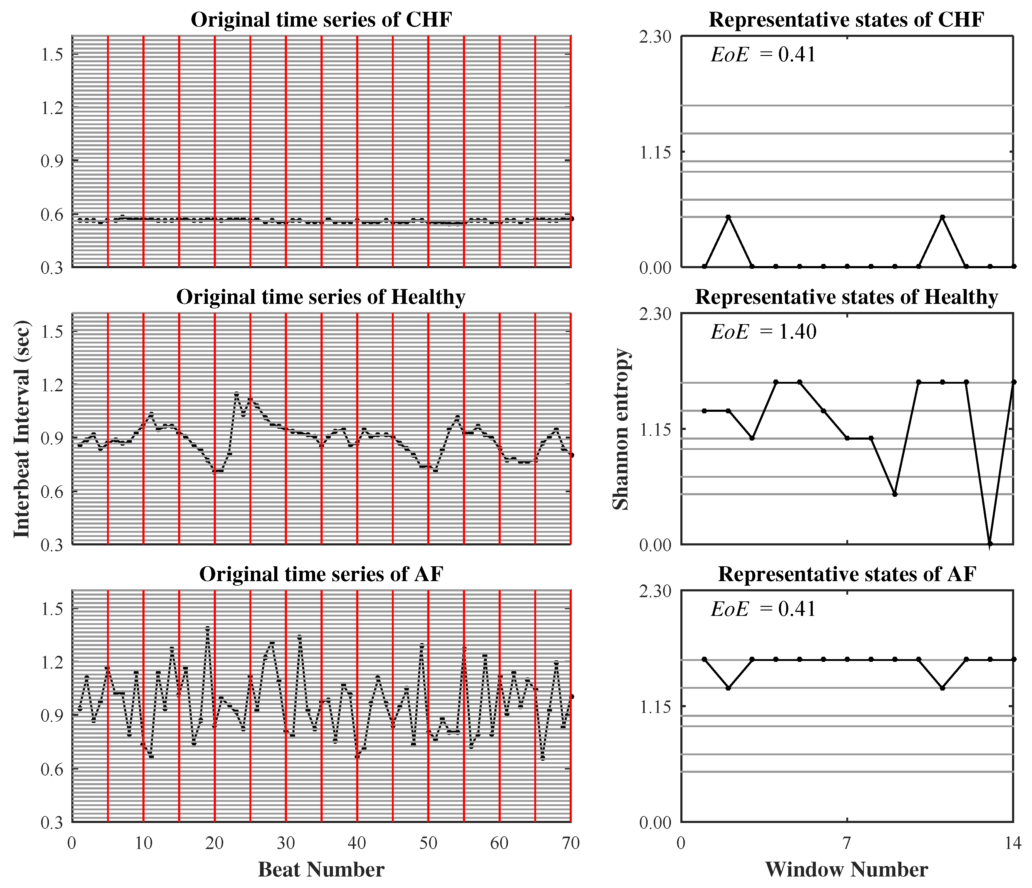
Figure 1 illustrates the two steps of the EoE method for three representative CHF, healthy, and AF time series of consecutive heartbeat intervals. Each series consists of 70 data points and is analyzed at . The resulting EoE values of the CHF, the healthy, and the AF are 0.41, 1.40, and 0.41, respectively. As expected, the EoE value of the healthy subject is significantly higher than those of the CHF and the AF.
3. Results
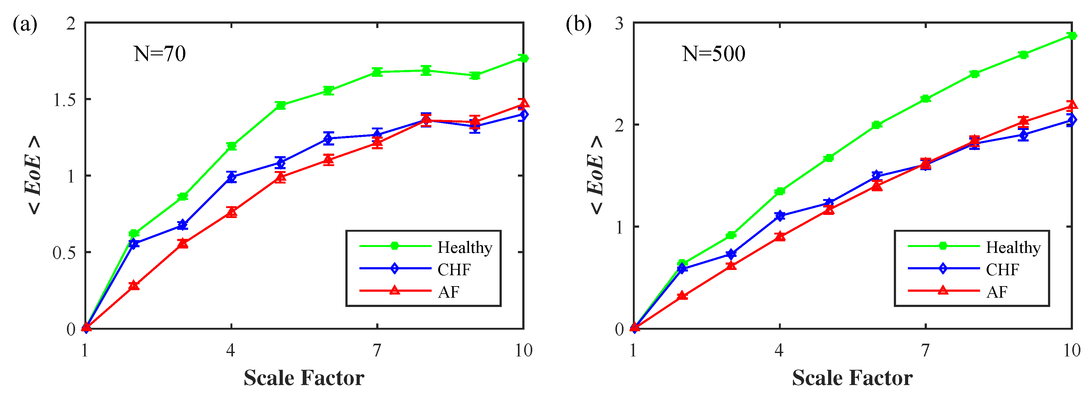
Figure 2 exhibits the average EoE values of the 237 selected sets of short time series from the healthy, the CHF, and the AF groups as a function of . The lengths N of the time series are (a) 70 and (b) 500, separately. For either length, all three <EoE> curves of the healthy, the CHF, and the AF monotonically increase with small . We find that the <EoE> of the healthy group remains higher than those of the two pathologic groups at all time scales, , and is significant for ≥ 5. Furthermore, the two pathologic groups of CHF and AF are not distinguishable.
3.1. Inverted U Curve
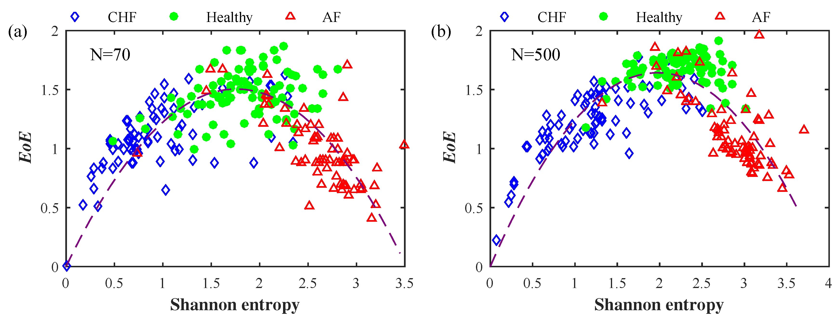
In order to present the three groups in a different manner, we plot the EoE at versus the Shannon entropy (of the original time series) with for each of the 237 sets of short time series with each of (a) 70 and (b) 500 data points, as shown in Figure 3. We observe that the CHF, the healthy, and the AF groups are spread and separated in three different regions: (1) the CHF group at the left-bottom region, (2) the healthy group at the middle-top region, and (3) the AF group at the right-bottom region. The whole distribution tends to form an inverted U shape.
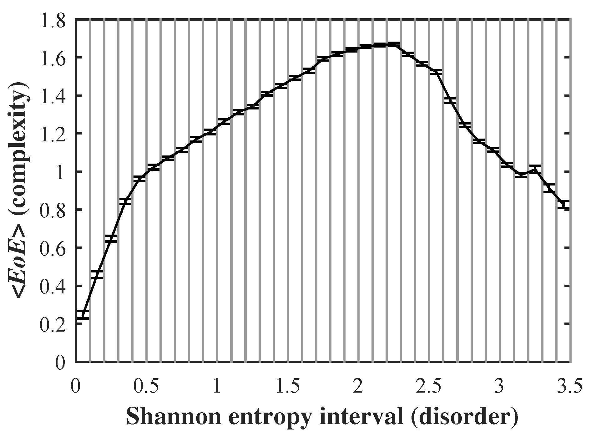
Furthermore, we apply this method to the three long-term databases (i), (ii), and (iii) as described above. Originally, there are 116 subjects taken into account. From each subject, we extract 100 short time series with each of 500 data points. In total, there are 11,600 sets of short time series. We first compute the EoE and the Shannon entropy of every series. Then, dividing the range of Shannon entropy from 0 to 3.5 into 35 equal intervals, we compute the mean value and standard error of those EoEs distributed over each interval. Figure 4 plots the average EoE values of each interval versus the corresponding Shannon entropy interval.
It is reasonable to characterize complexity with EoE and disorder with Shannon entropy of the original time series. Therefore, we illustrate the relationship between complexity and disorder as an inverted U shape where the maximal complexity value (as measured by EoE index) appears in the middle of extreme order and disorder. This finding is novel since it is consistent with the hypothesis in many studies on complexity [1,2,3,4,5,6,7,8] but has never been demonstrated in real data sets.
3.2. Accuracy of EoE
Table 1 lists the specificity of EoE on the Healthy group and the sensitivities of EoE on the congestive heart failure (CHF) as well as the atrial fibrillation (AF) groups for the 237 sets of short time series with each of 70, 300, and 500 data points, separately, at and . Here, the sensitivity and the specificity are defined as:
and
where TP is the number of the CHF or the AF subjects correctly classified as the CHF or the AF group, TN is the number of the NSR subjects correctly classified as the NSR group, FP is the number of the NSR subjects falsely classified as the CHF group, and FN is the number of the CHF or the AF subjects falsely classified as the NSR group.
The EoE threshold is obtained at the maximal accuracy of EoE in differentiating the healthy subjects from the two pathologic subjects of CHF and AF. The accuracy is defined as:
It can be seen that the longer the time series, the higher the sensitivities and the specificity of EoE. The overall sensitivities and specificity are comparable with those computed by other methods [8,20,21]. However, the EoE method is able to separate healthy subjects from CHF and AF patients at one time with less data points.
In terms of accuracy, it is worth noting that the competing method at the bed side are biochemical ones [22]. The accuracy of these bedside techniques is well above 0.95 in the diagnosis of congestive heart failure (CHF) in an urgent-care setting. Nevertheless, many of the entropy methods including the EoE analysis have the potential to be used at home care or remote area health care where there is no biochemical facilities available.
4. Discussion
4.1. Parameters and Setup
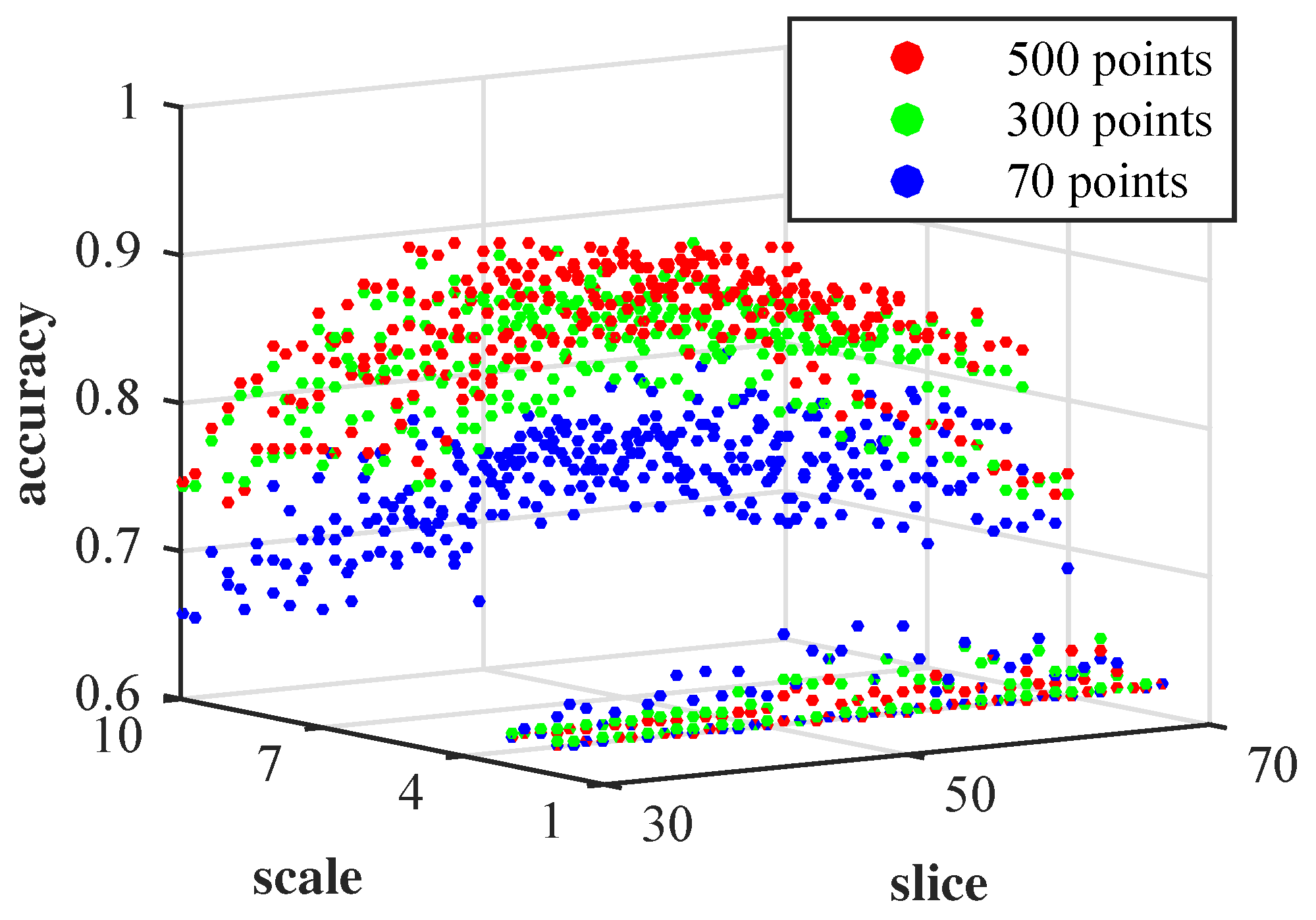
The accuracy of EoE depends upon the two parameters: the time scale and the number of slice . Figure 5 demonstrates a 3D plot of the accuracy of EoE as a function of and for the 237 sets of short time series with each of 70, 300, and 500 data points. It can be seen that there is a plateau in the central region of the graph, which is composed of a wide range of and s1 within a narrow range of accuracy. This implies that the results of our EoE analysis are robust with respect to the parameters and . This allows us to arbitrarily set = 55 near the center of the plateau in the previous work.
4.2. Simulated 1/f Noise and Gaussian Distributed White Noise
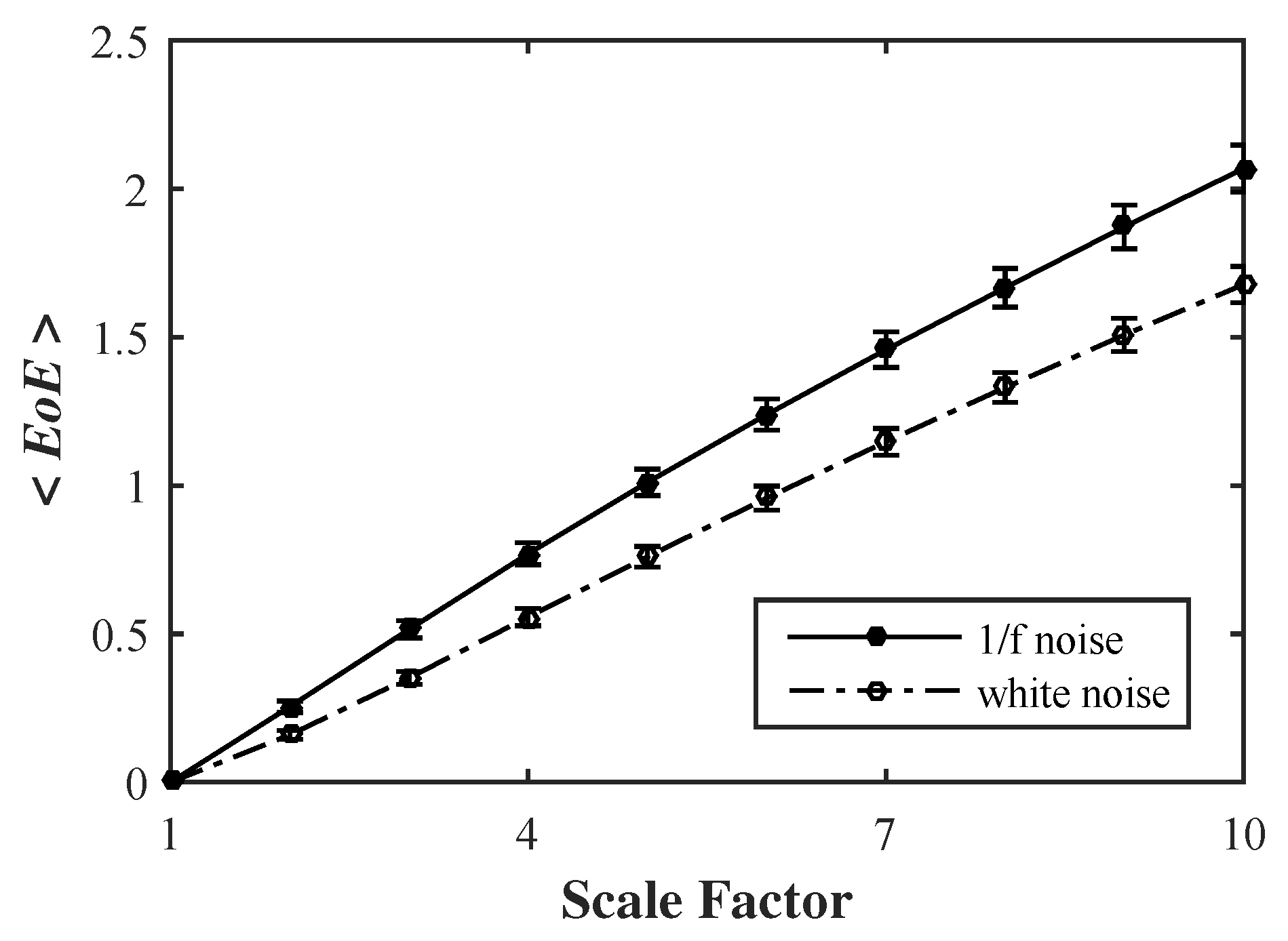
We also apply the EoE method to compute 100 simulated Gaussian distributed white noise and 1/f noise time series, with each of 5000 data points, individually. As shown in Figure 6, the average EoE values of the 100 1/f noise series are higher than those of the 100 white noise series for scales from 2 to 10 at .
4.3. Comparison between MSE and EoE
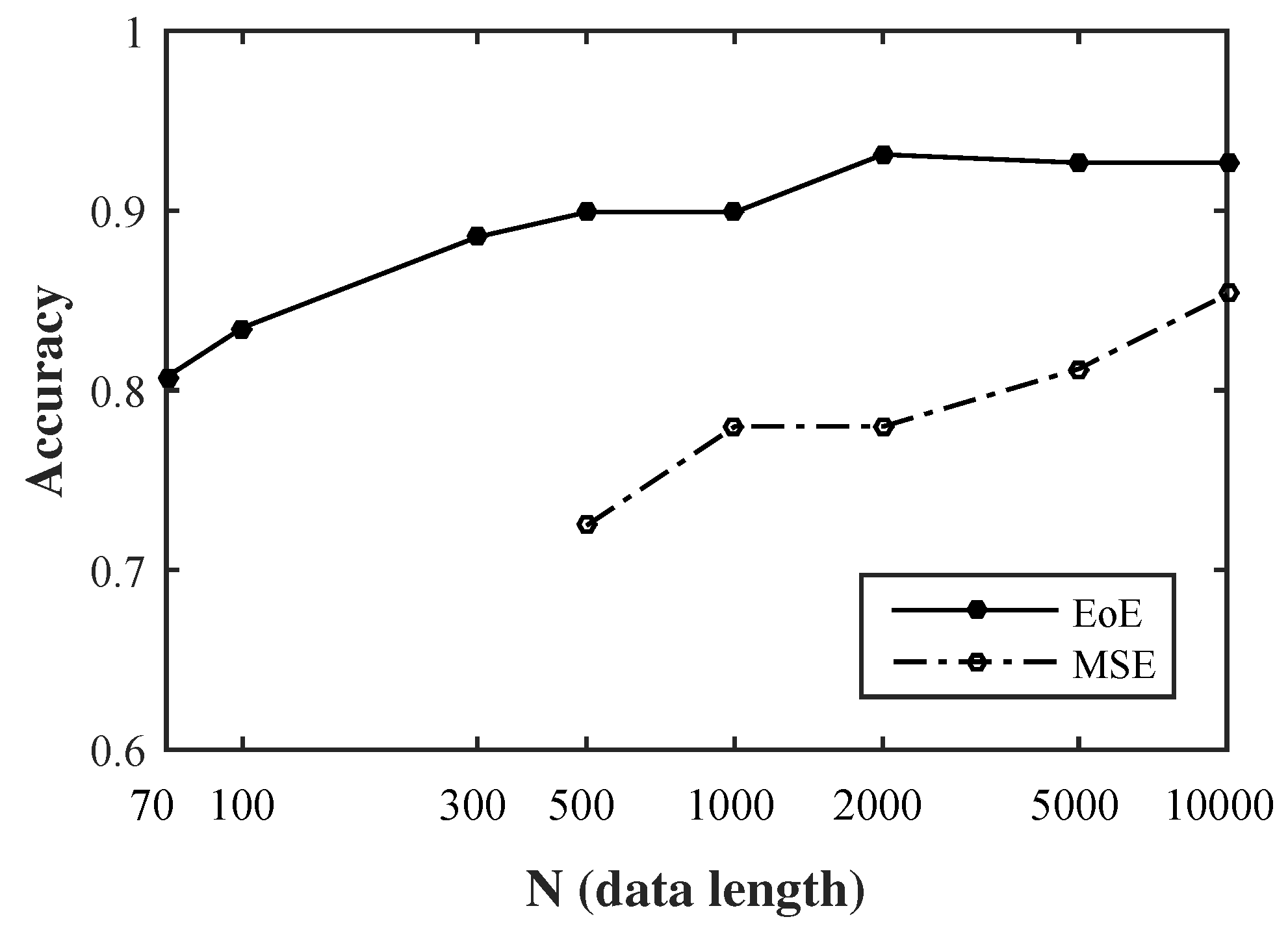
In separating the healthy group from the two pathologic groups of CHF and AF, MSE is most significant at among [2,3], while EoE is most significant for ≥ 5, as shown in Figure 2. We compare the accuracy of the MSE method at with that of EoE method at by applying them on the 218 sets out of the 237 selected sets of time series, whose lengths exceed 10,000 data points. The new database consists of 75, 90, and 53 sets from CHFDB, NSRDB, and LTAFDB, respectively. Figure 7 shows the relation between the relation between the accuracies of MSE and EoE methods on the 218 sets of short time series and the lengths of the time series that are extracted to range from 70 to 10,000.
It can be seen that the overall accuracy of EoE method is higher than that of the MSE method. In addition, short time series of 70 heart beats is sufficient for EoE analysis with an accuracy of 81% and longer series of 500 beats results in an accuracy of 90%. No reliable MSE result is available over the data lengths from 70 to 500 data points since the SampEn for irregularity in MSE requires a large amount of data points. Nevertheless, MSE provides more information in the profile of MSE curves in identifying a certain disease [23] than the complexity at alone as a general complexity used here.
The difference in effective data length between MSE and EoE methods may come from the different characteristics of the representative states defined in the first step of the two methods. This implies that there are multiple viewpoints to consider complexity of biological systems. Therefore, the application of either analysis depends upon the size and the kind of target physiologic time-series signal so as to better extract the complexity hidden inside.
5. Conclusions
Previously, MSE analysis was proposed as a measure of complexity that reflects the ability of a biological system to process complicated information so as to adapt and survive in an ever-changing environment [2,3,4]. MSE has been widely applied in analyzing many physiologic signals, such as heart rate [2,3,24], electroencephalography (EEG) signal [25,26,27], blood oxygen level-dependent signals in functional magnetic resonance imaging [28], diffusion tensor imaging (DTI) of the brain [29], neuronal spiking [30], center of pressure signals in balance [31,32] and intracranial pressure signal [33].
Following the same hypotheses proposed by the MSE analysis and the idea of superinformation for DNA sequences, we introduce EoE to characterize the complexity of a biological system from the viewpoint of the “variation of information” hidden in a physiologic time-series signal on multiple time scales. By computing Shannon entropy twice for a time series utilizing a multiscale approach, both the “information” and “variation” hidden inside the time series are extracted and interpreted as the ability of the system to adapt.
The advantage of the EoE analysis is that it can be applied to relatively short time series of 70–500 data points. The corresponding accuracy of EoE analysis ranges from 81% to 90%. This feature could be desirable in many applications where long time series are not available.
In addition, the EoE versus Shannon entropy plot of heart rate time series exhibits an inverted U relationship with the maximal EoE value appearing in the middle of extreme order and disorder, which has been previously hypothesized but never demonstrated in real data sets. Further exploration of the utility of this approach, by applying it to other heart beat databases and other physiologic signals, is needed for future work.
Acknowledgments
This work was supported by the Ministry of Science and Technology of the Republic of China (MOST104-2221-E009-132-MY3) and Delta Environmental & Educational Foundation, Taipei, Taiwan. We especially appreciate the Guest Editor for helping us with the coherence throughout the paper, which significantly improve the readability of our article. We also thank four reviewers whose valuable comments led to a much improved version of this paper.
Author Contributions
Chang Francis Hsu and Sien Chi conceived and designed the algorithm; Sung-Yang Wei and Han-Ping Huang analyzed the data; Long Hsu wrote the paper; Chung-Kang Peng provided advice and critical revision.
Conflicts of Interest
The authors declare no conflict of interest.
References
- Mitchell, M. Complexity A Guided Tour; Oxford University Press: Oxford, UK, 2009. [Google Scholar]
- Costa, M.; Goldberger, A.L.; Peng, C.-K. Multiscale entropy analysis of complex physiologic time series. Phys. Rev. Lett. 2002, 89, 68102. [Google Scholar] [CrossRef] [PubMed]
- Costa, M.; Goldberger, A.L.; Peng, C.-K. Multiscale entropy analysis of biological signals. Phys. Rev. E 2005, 71, 1–18. [Google Scholar] [CrossRef] [PubMed]
- Peng, C.-K.; Costa, M.; Goldberger, A.L. Adaptive data analysis of complex fluctuations in physiologic time series. World Sci. 2009, 1, 61–70. [Google Scholar] [CrossRef] [PubMed]
- Gell-Mann, M. What is complexity. Complexity 1995, 1, 16–19. [Google Scholar] [CrossRef]
- Huberman, B.A.; Hogg, T. Complexity and Adaptation. Physica D 1986, 22, 376–384. [Google Scholar] [CrossRef]
- Zhang, Y.-C. Complexity and 1/f noise. A phase space approach. J. Phys. I EDP Sci. 1991, 1, 971–977. [Google Scholar] [CrossRef]
- Silva, L.E.V.; Cabella, B.C.T.; Neves, U.P.D.C.; Murta Junior, L.O. Multiscale entropy-based methods for heart rate variability complexity analysis. Physica A 2015, 422, 143–152. [Google Scholar] [CrossRef]
- Beisbart, C.; Hartmann, S. Probabilities in Physics; Oxford University Press: Oxford, UK, 2011; p. 117. [Google Scholar]
- Shannon, C.E. Prediction and ntropy of printed english. Bell Syst. Tech. J. 1951, 30, 50–64. [Google Scholar] [CrossRef]
- Shannon, C.E. A Mathematical Theory of Communication. Bell Syst. Tech. J. 1948, 27, 379–423. [Google Scholar] [CrossRef]
- Pincus, S.M. Approximate entropy as a measure of system complexity. Mathematics 1991, 88, 2297–2301. [Google Scholar] [CrossRef]
- Richman, J.; Moorman, J. Physiological time-series analysis using approximate entropy and sample entropy. Am. J. Physiol. Hear. Circ. Physiol. 2000, 278, H2039–H2049. [Google Scholar]
- Chen, W.; Zhuang, J.; Yu, W.; Wang, Z. Measuring complexity using FuzzyEn, ApEn, and SampEn. Med. Eng. Phys. 2009, 31, 61–68. [Google Scholar] [CrossRef] [PubMed]
- Bandt, C.; Pompe, B. Permutation Entropy: A Natural Complexity Measure for Time Series. Phys. Rev. Lett. 2002, 88, 174102. [Google Scholar] [CrossRef] [PubMed]
- Porta, A.; Castiglioni, P.; Bari, V.; Bassani, T.; Marchi, A.; Cividjian, A.; Quintin, L.; DiRienzo, M. K-nearest-neighbor conditional entropy approach for the assessment of the short-term complexity of cardiovascular control. Physiol. Meas. 2013, 34, 17–33. [Google Scholar] [CrossRef] [PubMed]
- Hou, F.-Z.; Wang, J.; Wu, X.-C.; Yan, F.-R. A dynamic marker of very short-term heartbeat under pathological states via network analysis. Europhys. Lett. 2014, 107, 58001. [Google Scholar] [CrossRef]
- Bose, R.; Chouhan, S. Alternate measure of information useful for DNA sequences. Phys. Rev. E 2011, 83, 1–6. [Google Scholar] [CrossRef] [PubMed]
- BIDMC Congestive Heart Failure Database, MIT-BIH Normal Sinus Rhythm Database, and Long Term AF Database. Available online: http://www.physionet.org/physiobank/database/#ecg (accessed on 5 December 2016).
- VonTscharner, V.; Zandiyeh, P. Multi-scale transitions of fuzzy sample entropy of RR-intervals and their phase-randomized surrogates: A possibility to diagnose congestive heart failure. Biomed. Signal Process. Control 2017, 31, 350–356. [Google Scholar] [CrossRef]
- Liu, C.; Gao, R. Multiscale entropy analysis of the differential RR interval time series signal and its application in detecting congestive heart failure. Entropy 2017, 19, 3. [Google Scholar] [CrossRef]
- Dao, Q.; Krishnaswamy, P.; Kazanegra, R.; Harrison, A.; Amirnovin, R.; Lenert, L.; Clopton, P.; Alberto, J.; Hlavin, P.; Maisel, A.S. Utility of b-type natriuretic peptide in the diagnosis of congestive heart failure in an urgent-care setting. J. Am. Coll. Cardiol. 2001, 37, 379–385. [Google Scholar] [CrossRef]
- Lin, Y.H.; Huang, H.C.; Chang, Y.C.; Lin, C.; Lo, M.T.; Liu, L.Y.; Tsai, P.R.; Chen, Y.S.; Ko, W.J.; Ho, Y.L.; et al. Multi-scale symbolic entropy analysis provides prognostic prediction in patients receiving extracorporeal life support. Crit. Care 2014, 18, 548. [Google Scholar] [CrossRef] [PubMed] [Green Version]
- Costa, M.; Goldberger, A.L.; Peng, C.-K. Broken asymmetry of the human heartbeat: Loss of time irreversibility in aging and disease. Phys. Rev. Lett. 2005, 95. [Google Scholar] [CrossRef] [PubMed]
- Takahashi, T.; Cho, R.Y.; Mizuno, T.; Kikuchi, M.; Murata, T.; Takahashi, K.; Wada, Y. Antipsychotics reverse abnormal EEG complexity in drug-naive schizophrenia: A multiscale entropy analysis. Neuroimage 2010, 51, 173–182. [Google Scholar] [CrossRef] [PubMed]
- Garrett, D.D.; Samanez-Larkin, G.R.; MacDonald, S.W.S.; Lindenberger, U.; McIntosh, A.R.; Grady, C.L. Moment-to-moment brain signal variability: A next frontier in human brain mapping? Neurosci. Biobehav. Rev. 2013, 37, 610–624. [Google Scholar] [CrossRef] [PubMed]
- Liang, W.; Lo, M.; Yang, A.C.; Peng, C.; Cheng, S.; Tseng, P.; Juan, C. NeuroImage Revealing the brains adaptability and the transcranial direct current stimulation facilitating effect in inhibitory control by multiscale entropy. Neuroimage 2014, 90, 218–234. [Google Scholar] [CrossRef] [PubMed]
- Yang, A.C.; Huang, C.C.; Yeh, H.L.; Liu, M.E.; Hong, C.J.; Tu, P.C.; Chen, J.F.; Huang, N.E.; Peng, C.K.; Lin, C.P.; et al. Complexity of spontaneous BOLD activity in default mode network is correlated with cognitive function in normal male elderly: A multiscale entropy analysis. Neurobiol. Aging 2013, 34, 428–438. [Google Scholar] [CrossRef] [PubMed]
- Nakagawa, T.T.; Jirsa, V.K.; Spiegler, A.; McIntosh, A.R.; Deco, G. Bottom up modeling of the connectome: Linking structure and function in the resting brain and their changes in aging. Neuroimage 2013, 80, 318–329. [Google Scholar] [CrossRef] [PubMed]
- Bhattacharya, J.; Edwards, J.; Mamelak, A.N.; Schuman, E.M. Long-range temporal correlations in the spontaneous spiking of neurons in the hippocampal-amygdala complex of humans. Neuroscience 2005, 131, 547–555. [Google Scholar] [CrossRef] [PubMed]
- Wei, Q.; Liu, D.H.; Wang, K.H.; Liu, Q.; Abbod, M.F.; Jiang, B.C.; Chen, K.P.; Wu, C.; Shieh, J.S. Multivariate multiscale entropy applied to center of pressure signals analysis: An effect of vibration stimulation of shoes. Entropy 2012, 14, 2157–2172. [Google Scholar] [CrossRef]
- Kang, H.G.; Costa, M.D.; Priplata, A.A.; Starobinets, O.V.; Goldberger, A.L.; Peng, C.K.; Kiely, D.K.; Cupples, L.A.; Lipsitz, L.A. Frailty and the degradation of complex balance dynamics during a dual-task protocol. J. Gerontol.-Ser. A Biol. Sci. Med. Sci. 2009, 64, 1304–1311. [Google Scholar] [CrossRef] [PubMed]
- Lu, C.-W.; Czosnyka, M.; Shieh, J.-S.; Smielewska, A.; Pickard, J.D.; Smielewski, P. Complexity of intracranial pressure correlates with outcome after traumatic brain injury. Brain 2012, aws155. [Google Scholar] [CrossRef] [PubMed]
Figure 1.
Illustration of the two-step-operation of the entropy of entropy (EoE) method. The left column shows the three original heartbeat intervals time series of a congestive heart failure (CHF), the healthy, and the atrial fibrillation (AF) subjects with each of data points. First, each original time series is equally divided into 14 (=N/) windows of data points in red frames. The range of the interbeat intervals from to , derived from the three databases on PhysioNet, is equally divided into slices. This results in three coarse-grained sequences of 14 representative states in terms of Shannon entropy values as shown in the right column. Second, as illustrated by the grey lines in the right column, there are possible levels to accommodate all Shannon entropy values derived at . As a result, the Shannon entropy values of the three sequences from the CHF, the healthy, and the AF subjects are 0.41, 1.40, and 0.41, respectively. They are the EoE values of the three original time series.

Figure 2.
<EoE> vs. time scale at for the 90, 75, and 72 sets of short time series with each of (a) 70 and (b) 500 data points from the NSRDB, the CHFDB, and the LTAFDB. The separation of the healthy group from the two pathologic groups of CHF and AF is significant for ≥ 5. ( for the healthy and the pathologic group of CHF and AF; Student’s t-test). Symbols represent the mean values of <EoE> for each group and bars represent the standard error (, where n is the number of sets).

Figure 3.
EoE vs. Shannon entropy for the same 237 sets of short time series with each of (a) 70 and (b) 500 data points. The 75 diamond, 90 circle, and the 72 triangle symbols are from 15 CHF, 18 healthy, and 72 AF subjects. The EoE and the Shannon entropy are computed at and . In addition, the dashed line is a quadratic fitting.

Figure 4.
The inverted U relationship between (complexity) and Shannon entropy interval (disorder) associated with 11,600 sets of short time series from 116 subjects. The range of Shannon entropy from 0 to 3.5 is divided into 35 equal intervals. The mean and standard error of the EoEs distributed over each interval is computed. Note that the maximal EoE value appears in the middle of extreme order and disorder.

Figure 5.
EoE accuracy as a function of and for the 237 sets of short time series with each of 70, 300, and 500 data points. There is a plateau in the central region of the graph.
Figure 5.
EoE accuracy as a function of and for the 237 sets of short time series with each of 70, 300, and 500 data points. There is a plateau in the central region of the graph.

Figure 6.
EoE analysis of 100 simulated Gaussian distributed white noise and 1/f noise time series, with each of 5000 data points. Symbols represent the mean values of EoE for the 100 time series and error bars the SD.
Figure 6.
EoE analysis of 100 simulated Gaussian distributed white noise and 1/f noise time series, with each of 5000 data points. Symbols represent the mean values of EoE for the 100 time series and error bars the SD.

Figure 7.
The relationship between the accuracies of multiscale entropy (MSE) and EoE methods on the 218 sets of short time series and the lengths of the time series that are extracted to range from 70 to 10,000.
Figure 7.
The relationship between the accuracies of multiscale entropy (MSE) and EoE methods on the 218 sets of short time series and the lengths of the time series that are extracted to range from 70 to 10,000.


Table 1.
The specificity and the sensitivity of EoE method at = 5 and = 55.
| Date Length | 70 Points | 300 Points | 500 Points | |
|---|---|---|---|---|
| Group | ||||
| NSR (Specificity) | 0.86 | 0.93 | 0.91 | |
| CHF (Sensitivity) | 0.72 | 0.81 | 0.92 | |
| AF (Sensitivity) | 0.83 | 0.83 | 0.86 | |
a CHF: congestive heart failure group; b AF: atrial fibrillation group.
© 2017 by the authors. Licensee MDPI, Basel, Switzerland. This article is an open access article distributed under the terms and conditions of the Creative Commons Attribution (CC BY) license (http://creativecommons.org/licenses/by/4.0/).
Share and Cite
MDPI and ACS Style
Hsu, C.F.; Wei, S.-Y.; Huang, H.-P.; Hsu, L.; Chi, S.; Peng, C.-K. Entropy of Entropy: Measurement of Dynamical Complexity for Biological Systems. Entropy 2017, 19, 550. https://doi.org/10.3390/e19100550
AMA Style
Hsu CF, Wei S-Y, Huang H-P, Hsu L, Chi S, Peng C-K. Entropy of Entropy: Measurement of Dynamical Complexity for Biological Systems. Entropy. 2017; 19(10):550. https://doi.org/10.3390/e19100550
Chicago/Turabian StyleHsu, Chang Francis, Sung-Yang Wei, Han-Ping Huang, Long Hsu, Sien Chi, and Chung-Kang Peng. 2017. "Entropy of Entropy: Measurement of Dynamical Complexity for Biological Systems" Entropy 19, no. 10: 550. https://doi.org/10.3390/e19100550
Note that from the first issue of 2016, this journal uses article numbers instead of page numbers. See further details here.