Fault Diagnosis Using Improved Complete Ensemble Empirical Mode Decomposition with Adaptive Noise and Power-Based Intrinsic Mode Function Selection Algorithm

Abstract

In the fault diagnosis system using empirical mode decomposition (EMD), it is important to select the intrinsic mode functions (IMFs) which contain as much fault information as possible and to alleviate the problems of mode mixing and spurious modes. An effective solution to these problems in the decomposition process can help to determine significant IMFs and to improve the performance of the fault diagnosis system. This paper describes a novel power-based IMF selection algorithm and evaluates the performance of the proposed fault diagnosis system using improved complete ensemble EMD with adaptive noise and a multi-layer perceptron neural network.

1. Introduction

As malfunction of rotating machinery, which play an important role in industrial plants, can cause serious economic and personnel loss, efficient maintenance of machinery must be guaranteed. Generally, fault diagnosis techniques can be categorized into three main types in accordance with diagnostic procedures: model-based, signal-based, and data-based [1]. Signal processing is an indispensable part of these techniques because the purpose of the signal processing is to discover fault signatures from the measured data from machinery in operation.

Among the signal-based techniques for fault detection and diagnosis system, second-order cyclostationary is applied to the bearing and gearbox diagnostics and its effectiveness has been verified [2]. Cepstrum is known as a suitable technique for diagnostic purposes: the families of rahmonics are directly related to the frequency characteristics of rotating components [3]. The demodulation method has shown a high fault classification rate for spur gearboxes and improved for spiral bevel gearboxes diagnostics [4].

Even though these techniques provide satisfactory results, they are not appropriate enough for the analysis of nonlinear and non-stationary fault signals. Time–frequency analysis method is one of the most commonly used signal processing techniques due to its both time and frequency resolution at the same time. However, most of the existing time–frequency analysis methods decompose the signal based on a priori bases with assumption of the stationary signal. In contrast, wavelet transform and empirical mode decomposition (EMD) have effectively performed high resolution in both time and frequency domains, which have been successfully applied in faulty signal analysis. Continuous wavelet transform coefficients were used as features for the fault diagnosis system [5]. Wavelet packets decomposition (WPD), which takes advantage of effectively decomposing frequency bands into detail and approximate coefficients with multi-levels, has been applied to the fault diagnosis system [6]. Empirical mode decomposition (EMD), proposed by Huang et al., is an adaptive time–frequency analysis method and decomposes the signal into intrinsic mode functions (IMFs) that represent oscillation modes embedded in the signal and can serve as the basis functions derived from the signal itself. The EMD overcomes the intrinsic limitations of wavelet approach. EMD process is basically the analysis method generated by the same analyzed signal so setting the level of decomposition a priori is not required [7].

Although EMD is one of the best signal processing techniques, it still has unsolved problems due to the nature of the EMD: ‘mode mixing’ and ‘spurious modes’. To ameliorate mode mixing, ensemble EMD (EEMD), which employs an ensemble of noisy copies of the original signal in the decomposition, was proposed [8]. However, EEMD created new difficulties: the reconstructed signal contains residual noise and different realizations of signal plus noise can cause a different number of IMFs. The complementary EEMD (CEEMD) substantially alleviated the reconstruction problem using complementary pairs of noise [9], and the complete EEMD with adaptive noise (CEEMDAN) accomplished a negligible reconstruction error and solving the problem of different number of IMFs [10]. Colominas et al. proposed an improved CEEMDAN (ICEEMDAN) obtaining IMFs with less noise and more physical meaning [11].

Recently, a number of fault diagnosis based on EMD have been reported. Peng et al. suggested an improved Hilbert–Huang transform using wavelet packet transform and applied an IMF selection based on correlation coefficients [12] and Yu et al. proposed the concept of EMD energy entropy and utilized its value to identify different bearing fault types [13]. Junsheng et al. exploited singular values of IMFs as fault feature vectors of support vector machines [14] and Ricci et al. presented an automatic IMF selection method using a merit index [15]. Cho et al. proposed an IMF selection algorithm based on power–harmonic ratio (PHR) [16] and Lei et al. suggested a diagnosis method of rolling element bearings based on CEEMDAN [17]. Yi et al. presented an adaptive procedure based on EEMD and Hilbert marginal spectrum for multi-fault diagnostics of axle bearings and introduced the IMFs’ confidence index for automatic IMF selection [18]. Zhao et al. described a gearbox fault diagnosis approach that decomposes the signal using CEEMDAN and selects IMFs based on correlation coefficients and RP parameter [19]. Mohanty et al. compared four kinds of algorithm—FFT, EMD, EEMD, and CEEMDAN—to find out which algorithm is the best to avoid mode mixing problems and to enhance to the feature extraction and concluded that CEEMDAN is the most effective to extract the vibro-acoustic features [20].

In the EMD-based fault diagnosis, the IMF selection algorithm chooses the IMFs that contain the fault information and have the least influences of the mode mixing and spurious mode problems. If these problems are resolved successfully in the decomposition, the significant IMFs can be more distinguishable. Consequently, the IMF selection algorithm can be simplified and the performance of the fault diagnosis system will be improved. In this paper, a fault diagnosis system using a multi-layer perceptron (MLP), ICEEMDAN, and a novel power-based IMF selection algorithm is proposed.

2. Background: EMD, EEMD, CEEMD, CEEMDAN, and ICEEMDAN

2.1. EMD

The EMD method decomposes any type of signals into a small number of IMFs. The IMF is defined as a function with the following two conditions: (1) The number of extreme values and the number of zero crossings in the total data are the same or only one difference; and (2) at any point, the mean value of the envelope of the local minimum value and the envelope of the local maximum value is zero. From the definition of the zero crossing, the IMF has only one vibration mode, and the definition the IMF is not limited to a narrow band signal and can be of size and frequency modulation. In effect, this means a nonstationary condition. Therefore, one or more instantaneous frequencies may appear in arbitrary local time of complex data and EMD method is needed to analyze it. The EMD starts with three assumptions. (1) The signal has a minimum of two extremes. (2) The specific time scale is defined by the time lapse between extremes. Here, the specific time scale is an element that determines the vibration mode, i.e., the natural frequency. (3) If there are no extrema in the data and there is only a point of refraction, one or more differentiations can be performed to find the extrema. The crucial step in EMD is the sifting process. It is simply implemented by using envelope of the local maximum and the local minimum as the decomposition method by the IMF definition. Let x be the signal of interest. The algorithm can be described as follows:

• Set $k=0$ and find all extrema of $r_0=x$.
• Obtain the lower (upper) envelope $e_{min}\left(e_{max}\right)$ using interpolation function (cubic spline) for $r_k$ and compute the mean of the envelopes, $m=\left(e_{min}+e_{max}\right)/2$.
• Compute IMF candidate $h_1=r_k-m_1$ and repeat Step 1 to Step 2: $h_{11}=h_1-m_{11}$.
• Repeat $h_{1k}=h_{1\left(k-1\right)}-m_{1k}$ until the waveform is symmetric and find the first IMF $c_1=h_{1k}$.
• Compute the first residue $r_1=x-c_1$.
• Repeat Steps 1–5 to obtain the final residue $r_n$ until the residue $r_k$ satisfies some predefined stopping criterion: $r_1-c_2=r_1,\dots ,=r_{n-1}-c_n=r_n$.
• Finally, the signal $\mathrm{x}$ is decomposed into n number of IMFs and the residual signal $r_n$

  $$\mathrm{x}\left(t\right)={\displaystyle \sum }_{i=1}^n{c}_i+r_n.$$

  (1)

2.2. EEMD

Mode definition of the EEMD is the average of the corresponding IMFs obtained from an ensemble of the original signal adding different realizations of finite variance white noise. The algorithm can be described as follows:

• Generate $x^{\left(i\right)}=x+\beta W^{\left(i\right)}$, where $W^{\left(i\right)}$ is zero mean unit variance white noise realization, and $\beta >0$.
• Apply EMD process to each $x^{\left(i\right)},i=1,\dots ,L$ and then obtain the K number of modes $d_k^{\left(i\right)},k=1,\dots ,K$.
• Average the corresponding modes and assign the kth mode of $x$: ${\overline{d}}_k=\frac{1}{L}{\displaystyle \sum }_{i=1}^L{d}_k^{\left(i\right)}$.

In EEMD process, each $x^{\left(i\right)}$ is independently decomposed from the other realizations and residue $r_k^{\left(i\right)}=r_{k-1}^{\left(i\right)}-d_k^{\left(i\right)}$ is computed at each stage, but they are no connection between the different realizations. It causes two problems: (1) The signal is not completely decomposed; and (2) different realizations of the signal with noise could generate different number of modes.

2.3. CEEMD

The CEEMD was proposed to reduce reconstruction error. This model procedure is the same as EEMD but it adds noise to the original signal in pair (one positive and one negative) and generate two ensembles

$$\left[\begin{array}{c}{y}_1^{\left(i\right)}\\ y_2^{\left(i\right)}\end{array}\right]=\left[\begin{array}{cc}1& 1\\ 1& -1\end{array}\right]\left[\begin{array}{c}x\\ w^{\left(i\right)}\end{array}\right].$$

(2)

This method significantly reduces the residual noise in the reconstructed signal, but it still cannot overcome fundamental problems of the EMD process.

2.4. CEEMDAN

Let us define operators and symbols. $E_k\left(·\right)$ is the operator which produces the kth IMF obtained by EMD. The CEEMDAN algorithm can be described as follows:

• Decompose each $x^{\left(i\right)}=x+{\beta }_0{W}^{\left(i\right)}$ by EMD process, where $i=1,2,\dots ,L$ and compute its first mode: ${\tilde{d}}_1=\frac{1}{L}{\displaystyle \sum }_{i=1}^L{d}_1^{\left(i\right)}={\overline{d}}_1.$
• Compute the first residue at $k=1$: $r_1=x-{\tilde{d}}_1$.
• Generate the first mode of $r_1+{\beta }_1{E}_1\left(w^{\left(i\right)}\right)$, where $i=1,2,\dots ,L$ by EMD process and compute second mode: ${\tilde{d}}_2=\frac{1}{L}{\displaystyle \sum }_{i=1}^L{E}_1\left(r_1+{\beta }_1{E}_1\left(w^{\left(i\right)}\right)\right)$.
• Compute the kth residue, where $k=2,\dots ,\mathrm{K}$: $r_k=r_{\left(k-1\right)}-{\tilde{d}}_k$.
• Generate the first mode of $r_k+{\beta }_k{E}_k\left(w^{\left(i\right)}\right)$, where $i=1,2,\dots ,L$ by EMD process and compute the $\left(k+1\right)$th mode as

  $${\tilde{d}}_{\left(k+1\right)}=\frac{1}{L}{\displaystyle \sum }_{i=1}^L{E}_1\left(r_k+{\beta }_k{E}_k\left(w^{\left(i\right)}\right)\right).$$

  (3)
• Iterate Steps 4–5 until the residue cannot be decomposed by EMD process.

2.5. ICEEMDAN

Let us define new operators. $M\left(·\right)$ is the operator for calculating the local mean, for example, $E_1\left(x\right)=x-M\left(x\right)$, and $\langle$ is the operator averaging through the realizations. For the original CEEMDAN, the first IMF is $d_1=\langle E_1\left(x^{\left(i\right)}\right)\rangle =\langle x^{\left(i\right)}\rangle -\langle M\left(x^{\left(i\right)}\right)\rangle$. $std\left(·\right)$ means the standard deviation of the signal. ICEEMDAN algorithm can be described as follows:

• Generate $x^{\left(i\right)}=x+{\beta }_0{E}_1\left(W^{\left(i\right)}\right)$, where $i=1,2,\dots ,L$, ${\beta }_0={\epsilon }_0·std\left(x\right)/std\left(E_1\left(W^{\left(i\right)}\right)\right)$, and ${\epsilon }_0$ is the constant to control noise amplitude and a recommended value is 0.2 [8,21].
• Compute the local mean of L realization of Step 1 to obtain the first residue, $r_1=\langle M\left(x^{\left(i\right)}\right)\rangle$, and calculate the first IMF: $\widetilde{d_1}=x-r_1$.
• For $k=3,4,\dots ,K$, calculate the kth residue: $r_k=\langle M\left(r_{k-1}+{\beta }_{k-1}{E}_k\left(W^{\left(i\right)}\right)\right)\rangle$, where ${\beta }_k={\epsilon }_0·std\left(r_k\right),K\ge 1$.
• Compute the kth IMF:$d_k=r_{k-1}-r_k$.
• Iterate Steps 3–4 for next k.

3. Proposed Method

The aforementioned EMD-based or EMD variant-based techniques for fault detection and diagnosis has their own criteria to choose significant IMFs. There are four kinds of indicators composed of these criteria: (1) Correlation coefficient; (2) periodicity; (3) energy density; and (4) other specific factors such as skewness and harmonicity. These indicators can be used individually but are generally used in combination each other. As a matter of fact, the merit index [15] is a linear combination of the periodicity degree and absolute skewness value and the PHR [16] standing for the power–harmonic ratio employs the energy density of harmonics of both desired frequency peak and the target signal. The confidence index [18] is defined as an arithmetic between the correlation coefficient and specific indexes such as skewness, kurtosis, and impact allowance that applies the periodicity and maximum values. RP parameter [19] is related to both periodicity and energy density. These criteria have been developed to help the fault diagnosis system select desired IMFs automatically because the choice of the significant IMFs is generally realized by means of visual assessment or experience of the system operator.

Since the spurious mode problem is the nature of the EMD, this algorithm applied some complicated procedures to cope with this problem. In this paper, ICEEMDAN is employed because it significantly relieved both residue noise in IMFs and spurious mode problems. A novel and simple power-based IMF selection algorithm suitable for this environment is proposed and a summary of the algorithm is given as follows:

• Decompose the signal $x$ into IMFs using ICEEMDAN. Let obtained IMFs be $d_k$, $k=1,2,\dots ,K$.
• Compute the power of each IMF, $P_k={\displaystyle \sum }_{j=1}^N{\left|d_k\left(j\right)\right|}^2$, where N is the number of samples of each IMF.
• Rearrange powers in descending order, $P{D}_m=sort\left(P_k,\mathrm{Descending}\mathrm{order}\right)$, $m=1,2,\dots ,K$, and save the indexes of the rearranged powers as $P{I}_m$ = [k of the $P{D}_1$, k of the $P{D}_2$, …, k of the $P{D}_K$].
• Find the index indicating the biggest difference between $P{D}_m$: $\mathrm{v}=\mathrm{index}\left\{\max \left(\mathrm{diff}\left(P{D}_m\right)\right)\right\}$, where, $\mathrm{diff}\left(y\right)=\left|y_n-y_{n-1}\right|$.
• Finally, determine desired IMFs in the selected IMFs, $d_s$ where $s=P{I}_1,P{I}_2,\dots ,P{I}_v$ and $v\le K$.

4. Experiments and Results

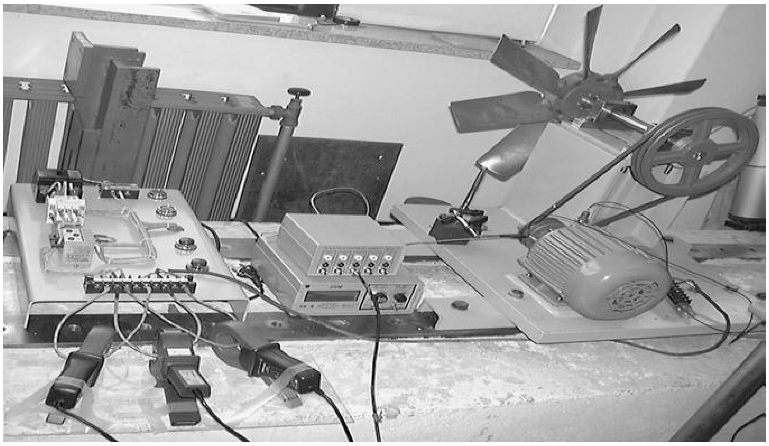
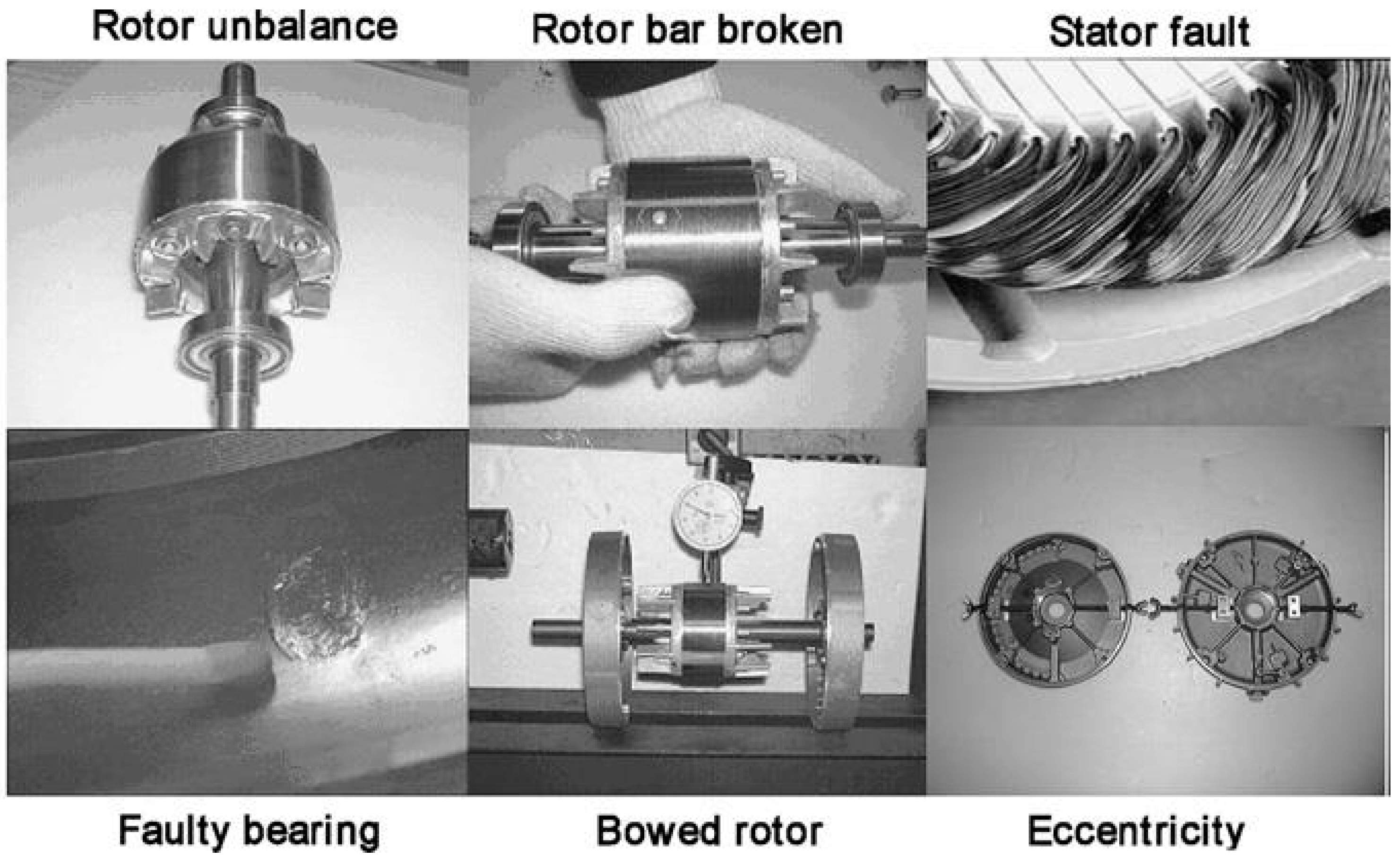
Figure 1 describes the overall proposed fault diagnosis system. The experiment is performed by using test equipment that contains a motor, pulley, belt, shaft, and fan with changeable blade angle that represents the load, as shown in Figure 2. To acquire the fault data, six induction motors (0.5 kW, 60 Hz, two-pole) are used under full load conditions. For the algorithm test, six conditions among eight categories are applied to the system. One of them is normal condition (NOR) to compare with five faulty motors: misalignment (MIS), rotor shaft (BRS), broken rotor bar (BRB), outer raceway faulty bearing (FBO), and rotor unbalance (RUN). The faulty conditions are described in Figure 3 and

Table 1. The description of faulty motors reproduced with permission from [22] Elsevier, 2018.

Fault Condition	Fault Description	Others
Broken rotor bar	No. of broken bar: 12 ea	Total number of 34 bars
Bowed rotor	Maximum bowed shaft deflection: 0.075 mm	Air-gap: 0.25 mm
Faulty bearing	A spalling on outer raceway	#6203
Rotor unbalance	Unbalance mass (8.4 g) on the rotor	5.48
Eccentricity	Parallel and angular misalignments	Adjusting the bearing pedestal
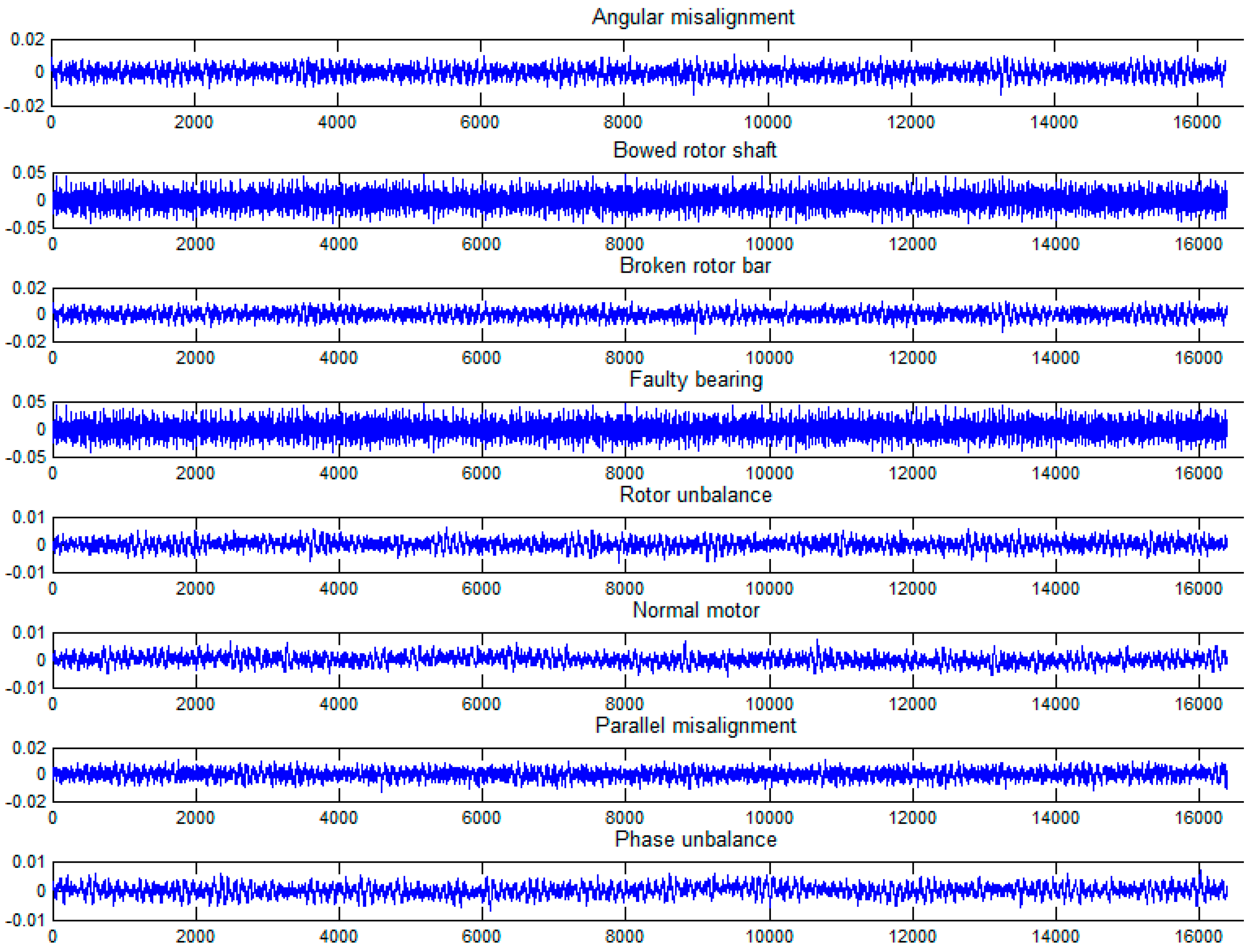
Phase unbalance	Add resistance on one phase	8.4%

and time domain presentation of each raw data is shown in Figure 4. Therefore, there are six kinds of fault categories and vibration data of each category motor are measured through accelerometers under 8 kHz sampling rate [22]. Acquired vibration signals have 12.29 s duration for each fault category. For ICEEMDAN, the vibration signals are divided into 2.05 s long signal. This process is performed 100 times randomly but the same signal is not generated. Finally, 100 data sets of each fault are produced.

In most previous studies, the number of desired IMFs used for fault diagnosis was determined by the length of the signal or user definition. In the case of the proposed algorithm, the criterion for the number of significant IMFs is basically provided as the length of s in the final step, but the value is not fixed. For the experimental data used in this paper, the length of s is 6 to 9. This paper uses the four most significant IMFs for fault diagnosis: $s=P{I}_1, P{I}_2, P{I}_3,P{I}_4$. This number is determined for objective comparison of the proposed algorithm with previous works.

For comparison to performance of the proposed IMF selection algorithm, time domain feature parameters—which Widodo et al. have proposed—are applied to the system and it uses two groups of feature vectors: nine features and four features for classification [22]. This is to compare the system classification performance according to the size of feature vectors and to inspect reliability of the proposed algorithm. One group includes RMS, variance, square root of amplitude (SRA), kurtosis value (KV), kurtosis factor (KF), skewness value (SV), skewness factor (SF), crest factor (CF), marginal factor (MF), and RMS. Another group contains variance, kurtosis value (KV), and skewness value (SV).

The purpose of the study is to evaluate the performance of IMF selection algorithm so that the influence of classifiers on the classification results can be minimized. Therefore, MLP neural network is applied as the classifier and the number of hidden layers are set to one based on universal approximation theory and it has three hidden neurons; the number of hidden neurons is determined based on the previous study [23]. The scaled conjugated gradient backpropagation is utilized as a learning algorithm and the learning threshold is defined as mean squared error, which is set to 1.00 × 10⁻⁵. This paper uses 100 data sets for each fault category; 70% for training data and 30% for test data, of which 20% is for validation. To prevent the over-fitting problem, 100-fold cross-validation was performed to achieve the exact classification. For comparison of system performance, EMD, EEMD, and ICEEMDAN are used as signal decomposition method and PHR-based method, and the proposed method is used as the IMF selection method with each signal decomposition method.

The classification results obtained from the proposed fault diagnosis system using nine features are given in

Table 2. Confusion matrix of classification results of the proposed fault diagnosis system using nine features (unit: %)

	Classification Results	MIS	BRS	BRB	FBO	NOR	RUN
Input Data
MIS		89.00	5.97	0.00	4.03	0.00	1.00
BRS		2.00	92.20	0.00	3.23	0.27	2.30
BRB		0.00	2.86	93.94	1.00	0.19	2.01
FBO		3.58	5.48	0.12	89.82	0.00	1.00
NOR		0.00	3.00	2.29	0.00	89.93	4.78
RUN		0.00	6.40	1.01	0.14	4.55	87.90

and show classification accuracy of about 88% to 94%. The accuracy of RUN is 87.90%, which is relatively low compared with the other fault classification accuracies, because the misclassification of RUN as BRS and NOR is as much high as 6.40% and 4.55%, respectively. Considering that RUN peaks at 1X component and spectra of BRS appears at 1X, 2X, and 3X and descend gradually, NOR and BRS are much similar signals to RUN than other fault signals.

Table 3. Comparison of performance for the fault diagnosis systems using nine features (unit: %)

	Methods	Proposed Method	ICEEMDAN + PHR	EEMD + Proposed	EEMD + PHR	EMD + Proposed	EMD + PHR
Factors
TACR		90.47	86..35	86.46	88.78	87.28	88.09
FN		5.01	10.24	7.42	10.16	14.43	14.26
NPV		94.72	89.07	91.42	89.47	85.64	85.99
PPV		98.01	96.73	95.92	97.28	97.21	97.50

describes the performance of the fault diagnosis systems using nine features in which diagnosis systems are the ICEEMDAN with proposed IMF selection (proposed method), ICEEMDAN with the PHR-based IMF selection (ICEEMDAN + PHR), EEMD with proposed IMF selection (EEMD + proposed), EEMD with the PHR-based IMF selection (EEMD + PHR), EMD with proposed IMF selection (EMD + proposed), and EMD with the PHR-based IMF selection (EMD + PHR), respectively. Comparison factors are total average classification rate (TACR), false negative (FN), negative predictive value (NPV) and positive predictive value (PPV). TACR is a factor that the system accurately diagnoses detected faults and PPV is a performance indicator that the system detects the fault itself. FN is defined as classifying the fault signal as a normal signal and the NPV is an index to represent that the results classified as normal are truly normal. Therefore, TACR and PPV represent the accuracy (or reliability) of the system, and FN and NPV are related to the stability of the system. For all comparison factors, the proposed system outperforms the other five systems. Considering TACR from the signal decomposition method point of view, PHR-based IMF selection method shows similar results regardless of the improvement of EMD performance. However, the proposed IMF selection performed the best performance at ICEEMDAN and it showed 3.18% improvement in performance compared to EMD. Considering FN in the same perspective, the excellence of proposed IMF selection method is clearly identified. Although PHR-based IMF selection improves signal decomposition performance from EMD to EEMD and ICEEMDAN, fault diagnosis system stays at approximately 4% performance improvement. On the other hand, changing EMD to ICEEMDAN in the proposed IMF selection method, it showed 9.42% system performance improvement. In NPV, the PHR-based and proposed IMF selection methods are improved by 3.88% and 9.08%, respectively. In PPV, the PHR-based and proposed IMF selection methods are improved by −0.77% and 0.8%, respectively. Consequently, the proposed IMF selection method contributes to improving the performance of the fault diagnosis system—improving its stability in particular— and the proposed fault diagnosis system has considerably improved performance and reliability compared to conventional systems.

Table 4. Comparison of performance for the fault diagnosis systems using four features (unit: %)

	Methods	Proposed Method	ICEEMDAN + PHR	EEMD + Proposed	EEMD + PHR	EMD + Proposed	EMD + PHR
Factors
TACR		90.22	88.16	83.08	83.86	84.21	84.66
FN		7.06	19.55	25.79	26.49	26.63	22.11
NPV		92.34	81.87	75.91	75.90	75.83	80.42
PPV		97.07	97.62	96.20	96.62	96.64	98.11

describes the performance of the fault diagnosis systems using four features. This is intended to determine how restricted the performance of each fault diagnosis system when the number of features is reduced. As a result, the results of the improvement of the classification performance and stability of the fault diagnostic system in the proposed algorithm appear almost identical to those described in Table 3.

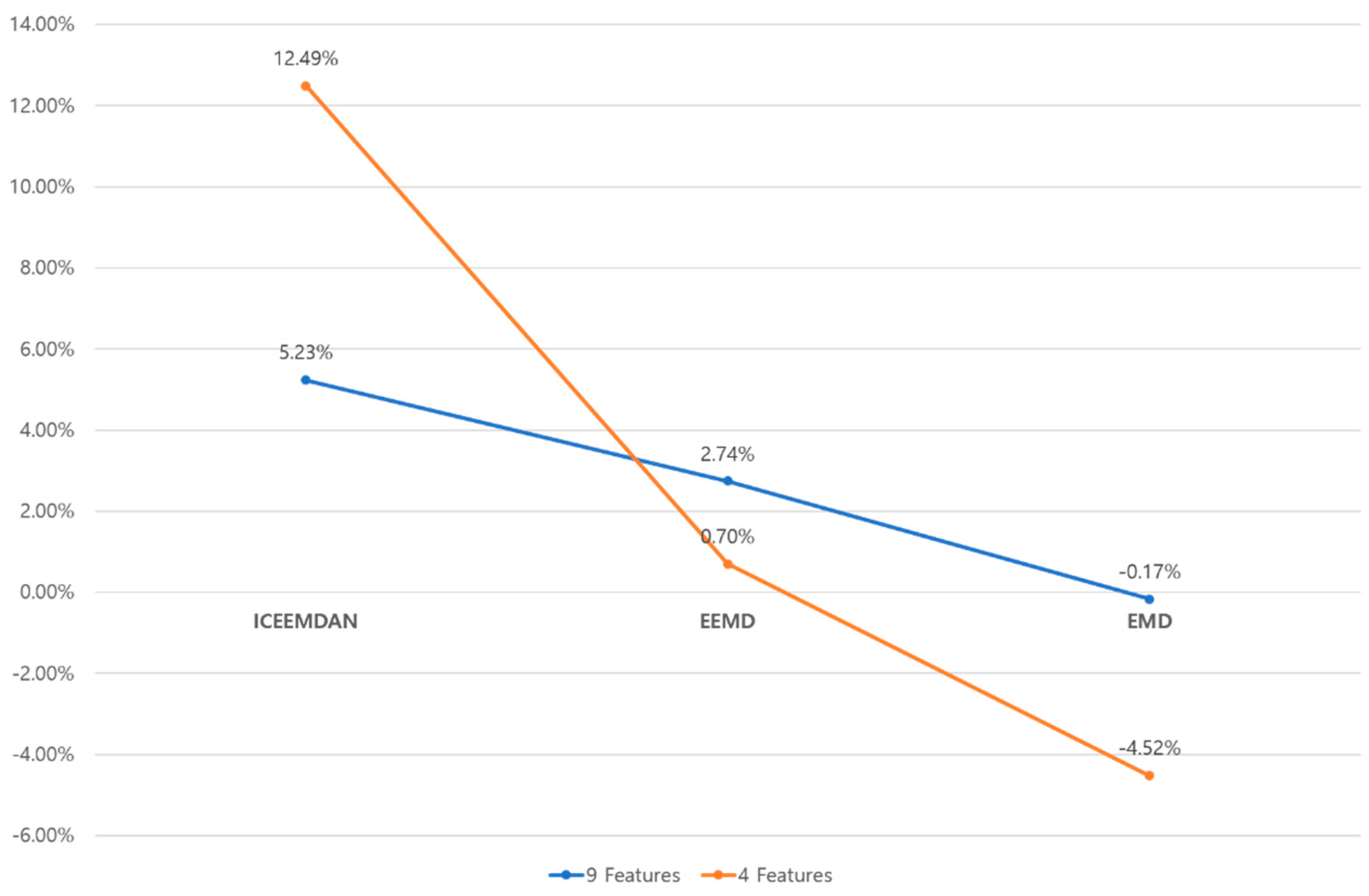
Figure 5 describes FN values according to IMF selection method. Applying the EMD, the PHR-based IMF selection showed superior performance regardless of the number of features, but applying EEMD and ICEEMDAN, the proposed IMF selection algorithm is far superior to the PHR-based IMF selection. In particular, it showed 12.49% performance improvement in the case using four features. This means that the proposed method is less sensitive to the number of features and contributes significantly to improving the performance of the system.

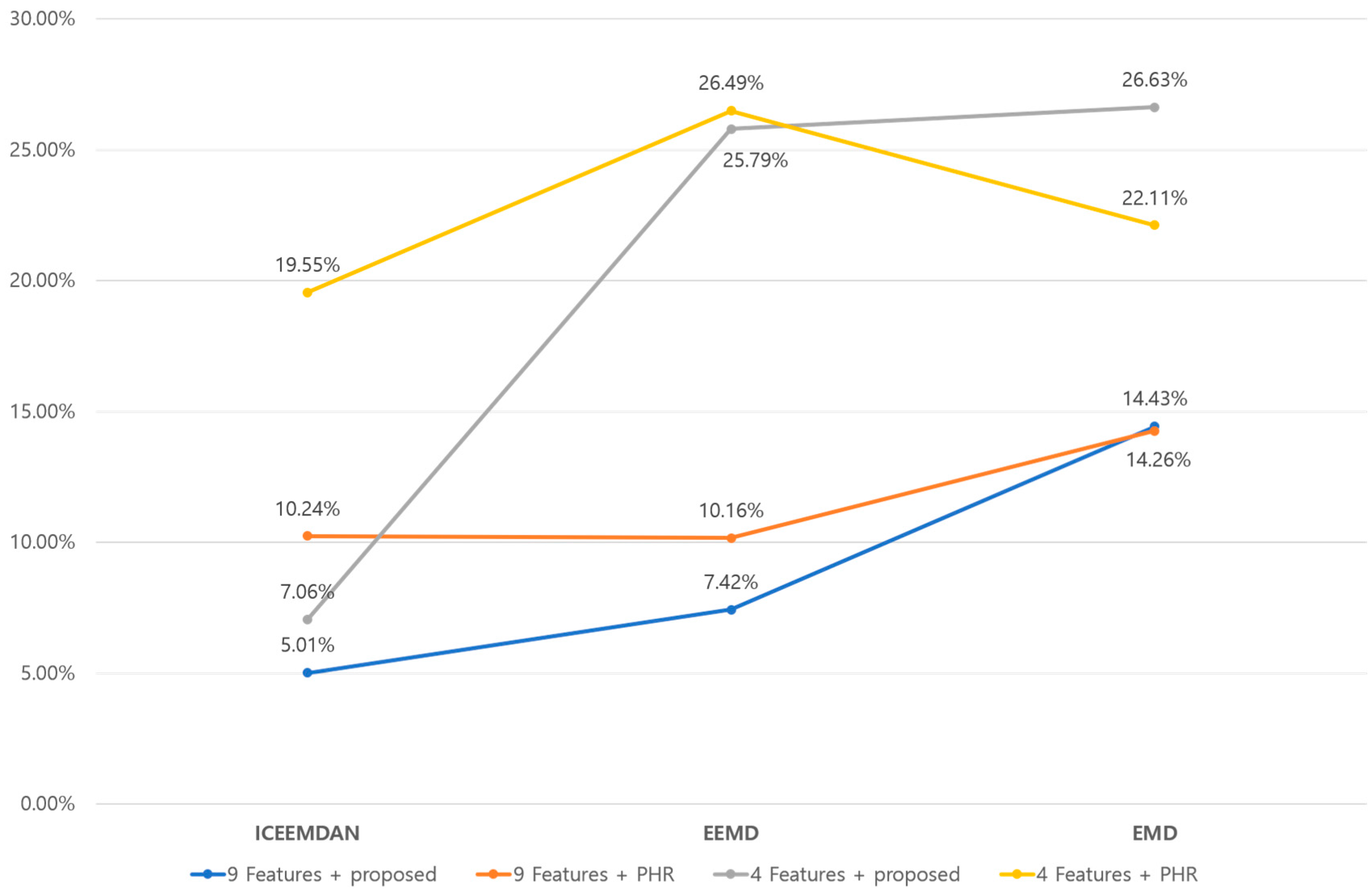
Figure 6 demonstrates FN values according to signal decomposition methods. While ‘9 Feature + PHR’ is improved 4.19% (14.43% to 10.24%), ‘9 Feature + proposed’ shows consistent improvement of 9.25% (14.25% to 5.01%). In other words, the PHR algorithm did not contribute much to improving performance in ICEEMDAN. In the case of four features, the proposed method gives significant improvement of 16.57% (26.63% to 7.06%). PHR shows a total 2.56% performance improvement but 4.38% performance degradation in EEMD. It is noteworthy that the system performance using the proposed algorithm increases proportionally to signal decomposition performance and shows significant performance improvements in the fewer features.

5. Conclusions

A fault diagnosis system using ICEEMDAN with the power-based IMF selection algorithm and the MLP is proposed and evaluated in this paper. The power-based IMF selection is not as complicated as the previous works and produces an appreciable performance improvement of the fault diagnosis system incorporating the proposed algorithm under ICEEMDAN. Laboratory experiments and analysis of results have confirmed the efficiency of the power-based IMF selection algorithm and have finally established that the proposed fault diagnosis system ensures high classification accuracy and stability against classifying faults as the normal state.

While EMD is based on a time–frequency analysis, many faults are easily detected by analyzing techniques in the frequency domain such that misalignment is 2/rev, shaft/motor imbalance is 1/rev, rotor bar is 60 Hz sideband of slip. However, the bearing fault only requires additional modeling for frequency such as envelope analysis, which means that without prior knowledge of a system, time–frequency analysis, ICEEMDAN + proposed IMF selection method is most appropriate for bearing analysis as there are cases where the fault frequencies are not known, as there is no bearing dimension information. Applying a model separating bearing cases from this proposed system, we expect to improve the performance of the proposed method much better.

Another main issue to apply the proposed system to an industrial field is that fault diagnosis should be performed with very unbalanced datasets, because it is not possible to obtain balanced datasets under real conditions. To solve this problem, Pedro proposed a rotation forest ensemble of C4.4 decision trees model for the gearboxes of wind turbines [24] and Luisa proposed an angular resampling algorithm [25]. Therefore, it is necessary to apply unbalanced datasets to the proposed system according to the proposed procedure. Recently, a lot of deep learning techniques have been proposed and applied to many fields such as image, voice, and text recognition or many prediction applications. These fields also deal with unbalanced dataset problems. Especially with recurrent neural network (RNN) and long-short term memory (LSTM), a more improved version of RNN is known as suitable method for one-dimensional time series data such as vibration. Applying RNN to the proposed method for an unbalanced test dataset will be important future work.