Bitcoin at High Frequency


1
Department of Economics and Business Economics, Aarhus University and CREATES, Aarhus BSS, Fuglesangs Allé 4, DK-8210 Aarhus V, Denmark
2
Tvilum A/S, Egon Kristiansens Allé 2, DK-8882 Faarvang, Denmark
*
Author to whom correspondence should be addressed.
J. Risk Financial Manag. 2019, 12(1), 36; https://doi.org/10.3390/jrfm12010036
Submission received: 12 December 2018
/
Revised: 23 January 2019
/
Accepted: 30 January 2019
/
Published: 15 February 2019
(This article belongs to the Special Issue Alternative Assets and Cryptocurrencies)
Abstract
:This paper studies the behaviour of Bitcoin returns at different sample frequencies. We consider high frequency returns starting from tick-by-tick price changes traded at the Bitstamp and Coinbase exchanges. We find evidence of a smooth intra-daily seasonality pattern, and an abnormal trade- and volatility intensity at Thursdays and Fridays. We find no predictability for Bitcoin returns at or above one day, though, we find predictability for sample frequencies up to 6 h. Predictability of Bitcoin returns is also found to be time–varying. We also study the behaviour of the realized volatility of Bitcoin. We document a remarkable high percentage of jumps above . We also find that realized volatility exhibits: (i) long memory; (ii) leverage effect; and (iii) no impact from lagged jumps. A forecast study shows that: (i) Bitcoin volatility has become more easy to predict after 2017; (ii) including a leverage component helps in volatility prediction; and (iii) prediction accuracy depends on the length of the forecast horizon.
1. Introduction
One of the reasons why cryptocurrencies—and in particular Bitcoin introduced by Nakamoto (2009)—became so popular in 2017 has been their huge price increase which caught the attention from both the media and regular people. Indeed, we find that approximately of all Bitcoin transactions happened in 2017 or later.1 As a consequence of this huge interest, Bitcoin experienced a price increase of 1324% from the begin to the end of 2017. The financial industry and the academics have also been very interested in Bitcoin over the last years. For example, the Chicago Mercantile Exchange (CME) as well as Nasdaq and the Tokyo Financial Exchange started to negotiate Bitcoin futures during 2017 and 2018, see CME (2017), Bloomberg (2017), and Cryptocoinsnews (2017). Academics working in the field of financial econometrics have studied Bitcoin using well known methodologies, such as ARMA–GARCH models. For example, Dyhrberg (2016) compared Bitcoin with gold and the American dollar and classified the behavior of Bitcoin in between these two assets. Bariviera (2017) found long memory in the Bitcoin volatility measured as the logarithmic difference between intraday highest and lowest prices. Phillip et al. (2018) document long memory in cryptocurrencies as well. Additional results about the time–dependence properties of cryptocurrencies are reported in Zhang et al. (2019). Ardia et al. (2018) and Stavroyiannis (2018) model and forecast the value at risk for Bitcoin. Recently, Catania and Grassi (2017) show that standard volatility models, like GARCH, are generally not suitable for cryptocurrency time–series and suggest to use a more sophisticated modelling technique based on the score driven approach, see Creal et al. (2013) and Harvey (2013). The predictability of cryptocurrencies returns and volatility has been studied in Catania et al. (2019) and Catania et al. (2018), respectively. Understanding the behavior of Bitcoin volatility has important implications for individual investors and public institutions. Individual investors – people not in the finance industry but interested in trading cryptocurrencies – should be informed about how the Bitcoin volatility evolves and whether these investment opportunities match with their risk profile. Public institutions, like the central banks of Ecuador, Tunisia, and Sweden who are considering issuing their own cryptocurrency, should be interested in the behavior of Bitcoin due to the possible systemic risk they would face by entering in this new market.
In this paper, we study the Bitcoin returns at high frequency and its realized volatility measure. We start by describing the construction of our dataset from the raw transactions downloaded from the Bitstamp and Coinbase exchanges.2 The first part of our analysis focuses on the in sample properties of Bitcoin returns sampled at different frequencies. We study the autocorrelation structure of Bitcoin returns as well as the intraday and intraweek seasonalities of Bitcoin volatility and traded volumes. Results indicate strong presence of both intraday and intraweek seasonality in the volatility. We also document that seasonality is different across exchanges. Specifically, Coinbase follows the US trading activity, while Bitstamp the European one. The second part the paper focuses on predicting realized volatility for Bitcoin using several forecasting models. Realized volatility is a consistent estimator of the quadratic variation of the price process and is presently widely used in financial and risk management applications, see Bauwens et al. (2012) for a recent overview. We consider the baseline HAR-RV model of Corsi (2008) as well as its generalization with the inclusion of jumps (Andersen et al. 2007; Barndorff-Nielsen 2004; Barndorff-Nielsen and Shephard 2003; Barndorff-Nielsen et al. 2006) and the leverage component (Corsi et al. 2012). Our results suggest that: (i) the predictability of Bitcoin realized volatility has increased over time; (ii) including the leverage component helps in predicting future volatility levels; and (iii) predictability varies with the forecast horizon. Both in sample and out of sample results are reported for the two exchanges as well as for the subperiod 2017–2018 which coincides with the explosion in the interest of Bitcoin. Overall, our results indicate several peculiarities of Bitcoin volatility compared to the volatility of alternative investment opportunities. First, we find that the frequency of jumps is much higher compared to common findings. Second, in contrast to Catania and Grassi (2017) and Ardia et al. (2018) who find an “inverted” leverage effect, our results show that Bitcoin exhibits a leverage effect similar to that of equity assets when this is measured using the Realized Volatility estimator. This last point also supports the arguments of Dyhrberg (2016) who classify Bitcoin as an asset and not as an exchange rate. Indeed, the leverage effect is of little importance for exchange rates as documented for example by Hansen and Lunde (2005) and Ardia et al. (2018).
The structure of the paper is organized as follows. Section 2 details the dataset we build starting from tick–by–tick price changes to equally spaced logarithmic returns. Section 3 studies the behaviour of Bitcoin returns sampled at different frequencies. Section 4 analyses the realized volatility of Bitcoin. Conclusions are drawn in Section 5.
2. Data
Our dataset is composed by tick-by-tick traded prices recorded at the two exchanges Bitstamp and Coinbase over which the majority of the transactions takes place. From both exchanges we collect the tick-by-tick transaction data using the freely available API at www.api.bitcoincharts.com. The raw data include the transaction price for every trade, along with the amount of Bitcoins traded. Observations start the 13 September 2011 on Bitstamp and the 1 December 2014 on Coinbase and are reported in UTC time. We record data up to 18 March 2018 for a total of 22,457,894 trades for Bitstamp and 39,439,004 for Coinbase. Unfortunately, trades are reported with a precision of one second. However, even though it is not reported in the exchanges documentations, we conjecture that trades within a second are reported in a chronological order. Overall, we find that 47.35% and 70.40% of the recorded transactions happen simultaneously with at least one other trade for Bitstamp and Coinbase, respectively.
Data Cleaning
Similar to standard high-frequency financial time-series, raw tick-by-tick Bitcoin prices are contaminated by wrongly reported observations. As suggested by Barndorff-Nielsen et al. (2009), we start by removing all those transactions associated with zero or negative volume. As a second step of data cleaning, we apply the methodology of Brownlees and Gallo (2006) to filter each transaction price. Specifically, let be the price of Bitcoin associated with trade i in our dataset, we apply the following rule:
where and denote -trimmed mean and sample standard deviation of a neighborhood of k observations around i, respectively. According to Brownlees and Gallo (2006), the positive integer k should be chosen as a function of the trading intensity, which for Bitcoin is relative high since there is no minimum buy-level. The additional tuning parameter is a granularity parameter and should prevent a zero standard deviation caused by sequences of k equal prices. Finally, helps to reduce the effect of extreme observations during the filtering procedure. We run the filter reported in Equation (1) using different choices of , and k. Table 1 reports results from the cleaning procedure in terms of percentage of outliers eliminated over the full sample and on a daily basis, for different choices of the tuning parameters and . We set and found that results are robust to this choice.
The percentage of outliers we find are consistent with the findings of Brownlees and Gallo (2006) and Barndorff-Nielsen et al. (2009). For and we find almost half the amount of outliers than for the case and . In general, we see a clear decreasing pattern in the amount of outliers when increasing the surrounding neighborhood as well as the granularity parameter. Consistently with Brownlees and Gallo (2006), we also find that the amount of outliers increases along with the increase in the number transactions. Indeed, for the case and , we find that 58.66% and 81.95% of the outliers are from 2017 or later for Bitstamp and Coinbase, respectively. Generally, we find that the outcome of the cleaning procedure is similar to that of Brownlees and Gallo (2006) suggesting that no particular attention should be made when dealing with high-frequency Bitcoin prices compared to the standard procedure employed for other financial series. Therefore, we stick to Brownlees and Gallo (2006) and use price series filtered using for our analysis. Starting from the filtered series of prices, we compute an equally spaced sequence of one–second prices and volumes. When multiple transactions are available within the same second, we set the final price to the median price computed over that second. Days with less then 40 observations have been removed for the dataset. We removed 167 days for Bitstamp and 16 days for Coinbase from the begin of the sample. Beside this, in order to remain with a time series without missing days, we let our data set to start from 17 March 2013 for Bitstamp and from 2 February 2015 for Coinbase. In order to isolate the effect of 2017, for the rest of the paper results are reported for the full sample as well as for the sub-sample after 1 January 2017 at midnight labelled as “Hype”. Table 2 summarizes the results from the cleaning procedure.
3. High Frequency Bitcoin Returns and Realized Volatiltiy
We start our analysis by computing the series of percentage Bitcoin logarithm returns at second in day t as:
where and are two subsequent Bitcoin prices for day t. One second logarithmic returns are subsequently aggregated at different frequencies as reported below. We also compute the realized volatility for day t as in Andersen et al. (2001b). As suggested by Liu et al. (2015) realized volatility is computed using 5-min returns, as:
where and and and we set to achieve 5-min. aggregation. Table 3 reports a comparison between the realized variance of Bitcoin and the variance of S&P 500 measured with the VIX. We note that the volatility of Bitcoin and that of S&P 500 are comparable during the years 2015 and 2016. On the contrary, in the period 2017–2018 the volatility of Bitcoin is considerably higher compared to that of S&P 500. We also note that volatility of Bitcoin is higher during the bear market period of 2018 than during the bubble period of 2017. Overall, results indicate that the volatility of volatility is much higher for Bitcoin than for the S&P 500.
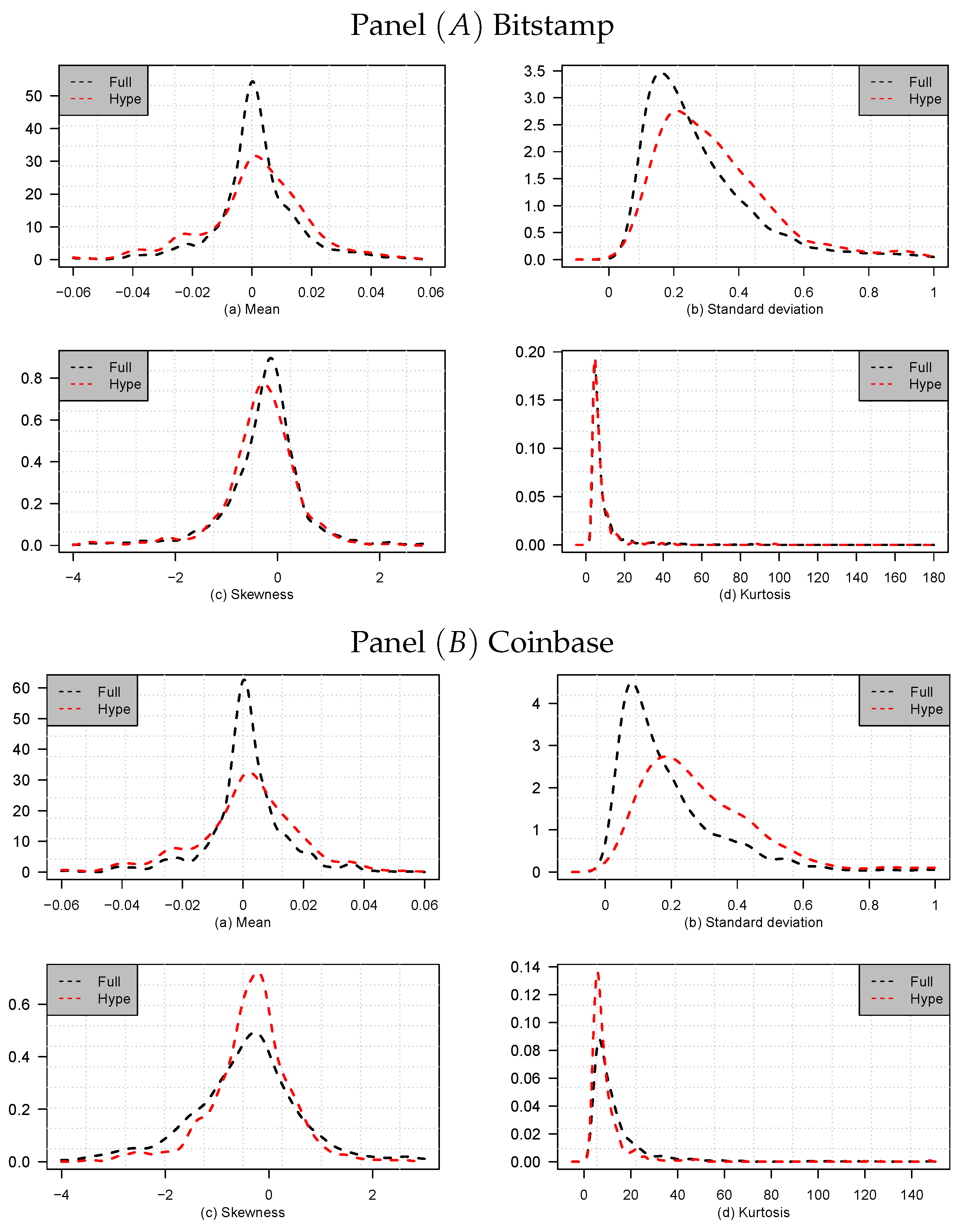
Descriptive statistics for Bitcoin percentage log returns aggregated at the 5-min. frequency are reported in Table 4. We observe that both series are characterized by extreme observations. We find that returns traded at the Bitstamp exchange exhibit higher volatility. However, we also note that returns traded at Coinbase are characterized by more pronounced negative skewness and higher excess of kurtosis. Overall, departure from Gaussianity is evident from the data. To conclude the analysis of Bitcoin returns at 5-min, in Figure 1 we report Gaussian kernel densities estimated on the mean, standard deviation, skewness, and kurtosis coefficients computed over each trading day available in our dataset. Interestingly, while the skewness and the excess of kurtosis coefficients are similar across exchanges and sub–samples, we note that the distribution of the standard deviation is considerably shifted to the right during the Hype period. Furthermore, it is also evident that during the Hype period we observe more dispersed average returns.
3.1. Are Bitcoin Returns Predictable?
Catania et al. (2019) investigate the predictability of Cryptocurrencies returns—and in particular Bitcoin—at one–day horizon.3 They find evidence of predictability for Bitcoin returns at the one–day frequency when averaging over a large number of Dynamic Linear Models resorting to the Dynamic Model Averaging technique. In this section, we only focus on the plain autoregressive model of order one defined as:
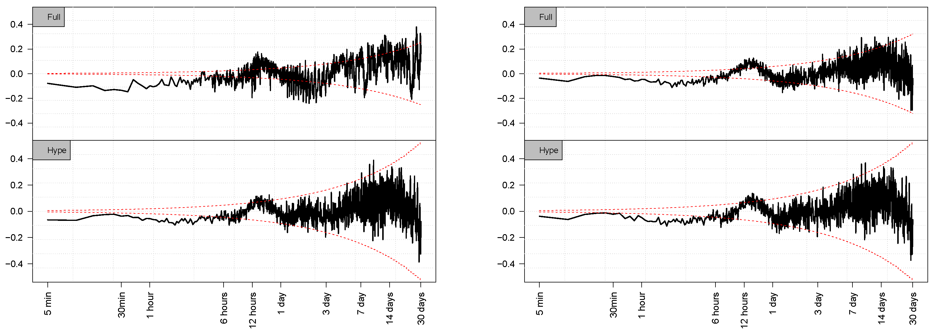
where is the first order autoregressive coefficients for frequency N. Figure 2 plots the estimated coefficient for Bitstamp and Coinbase according to different values of N starting from (five minutes) to (30 days). Results for the Hype period are also reported. We find that is negative and statistical different from zero when returns are aggregated up to 6 h. The autoregressive coefficient follows an upward trend and a peculiar curve around the 12 h aggregation frequency. After this point, the estimated coefficient decreases again and start being quite noisy around 0. We find that this behaviour is consistent across exchanges and also holds during the Hype sub-sample.
We conclude that there is no strict evidence indicating that Bitcoin returns can be predicted using a first order autoregressive model when looking at horizons longer than a day. However, by looking at intraday horizons, and especially within the first 6 hours, it seems like there is some predictability, even though the statistical significance is limited.4
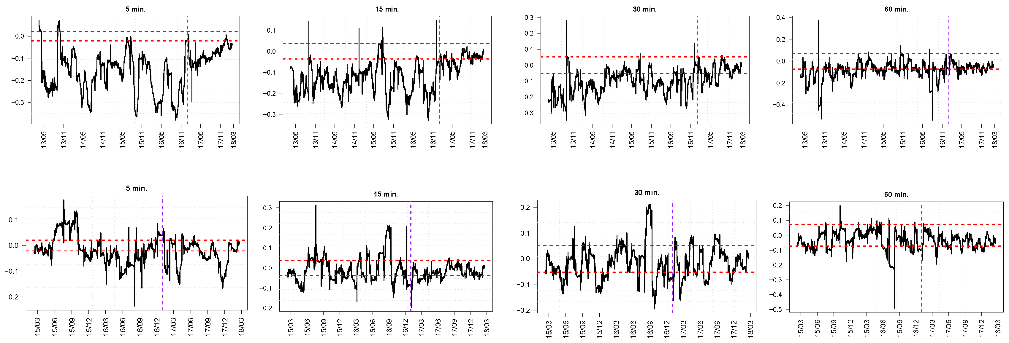
Gencay et al. (2001) note that the first order autocorrelation of high frequency financial assets is time–varying resulting in different patterns of predictability over time. We follow their approach and investigate the stability of the estimated over time for different N. We expect that due to the increase in the number of transactions the Bitcoin market has become more efficient over time, resulting in insignificant predictability based on prior observations. Thus, we estimate for (15 min), (30 min), and (one hour) using only observations available in the previous month of data and update its value according to a rolling window of fixed length. Figure 3 displays the estimated coefficients for Bitstamp and Coinbase. We find that during the begin of the sample Bitstamp shows a significant predictability pattern for both the 30 min and one hour intervals. Though, from the beginning of 2015, this predictability seems to have shrinkage down and lead into the 95% confidence range indicating insignificant predictability. This pattern indicates that Bitcoin traded at Bitstamp has become more efficient especially during the Hype period. Differently, in the Coinbase exchange we do not find the same predictability pattern. A possible explanation could be the more substantial amount of trades for the Coinbase exchange compared to Bitstamp, which implies that Coinbase is a more liquid and efficient market.
3.2. Seasonality in Bitcoin’s Volatility
Similar to foreign exchange rates, also Bitcoin exhibits a large amount of seasonality in its volatility, see for example Dacorogna et al. (1993), Taylor and Xu (1997), and Breedon and Ranaldo (2013). We investigate the daily seasonality pattern by looking at the intraday realized volatility computed at 30 min over the full sample and over the Hype period, as well as the average traded volumes computed at the same frequency.
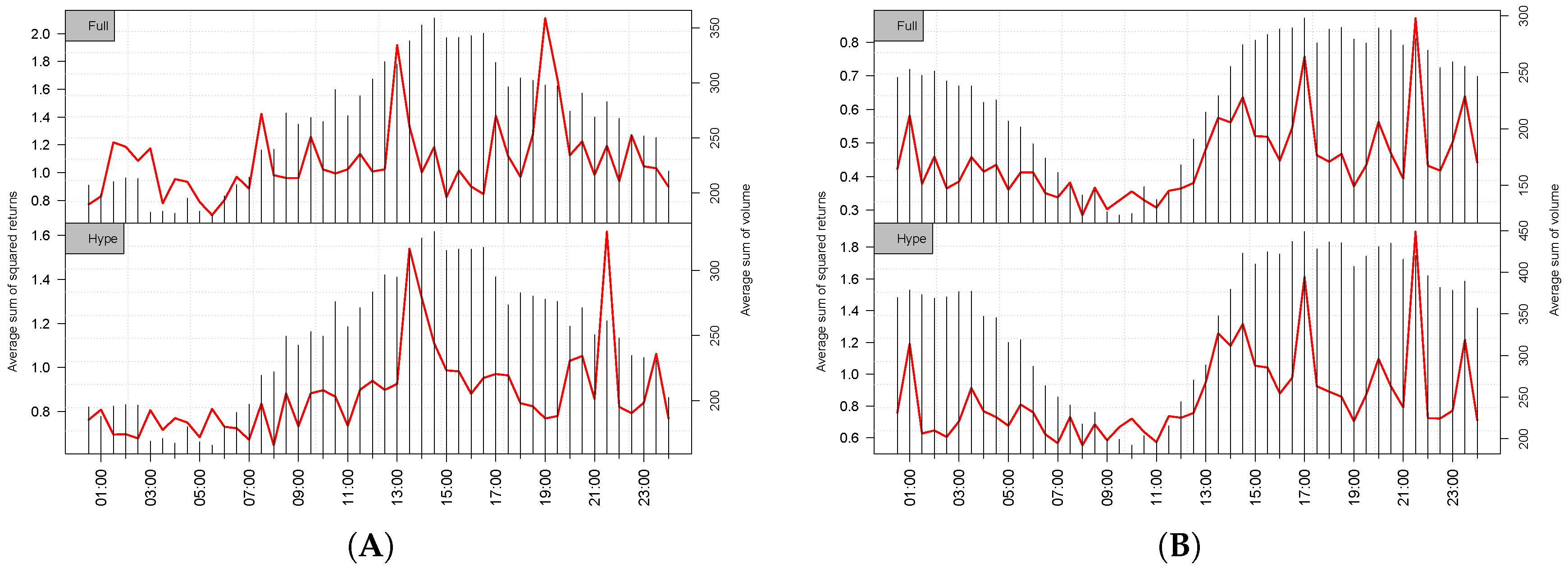
Figure 4 reports a graphical illustration of the intraday realized volatility and average volumes every 30 min. The figure shows a clear seasonality pattern for the average traded volume (vertical lines) and intraday realized volatility (red line). It is interesting to see the differences in the two exchanges peak hours, referring to the fact that Bitstamp is a European-based exchange, and Coinbase is a US-based exchange. Hence, they have spikes in different timezones associated with their working hours. Asia should be represented in both exchanges but does not seem to influence the two figures. We also note that the seasonal pattern has not changed during the Hype period.
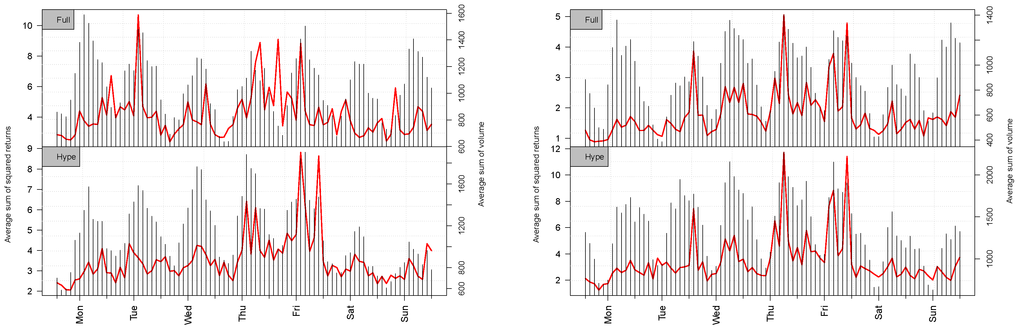
Besides the analysis of the intra-daily seasonality, we also investigate whether there is presence of intra-weekly seasonality. Following Dacorogna et al. (1993), we divide the week into a sequence of 2 h equally spaced observations. Figure 5 reports the weekly sequence based on average realized volatility (red line) and the average sum of volume (vertical lines). The effect of the weekends is clear from the figure. However, we note that this effect is more pronounced during the Hype period reported in the top panel of the figure. Interestingly, we also find evidence of intra–weekly seasonality for other days. Indeed, for both the exchanges we observe increasing activity from Monday to Thursday–Friday and then a decreasing curve over Saturday and Sunday. Remarkably, this effect during working days is not present for regular financial trading assets.
4. Modelling and Predicting Bitcoin Realized Volatility
In this section, we report on an in sample and out of sample forecast analysis of the Bitcoin’s realized volatility using several Heterogeneous Autoregressive (HAR) specifications. HAR has been originally introduced by Corsi (2008) in order to approximate the slow decay of the autocorrelation function of realized volatility. The model builds on the assumption of three different types of investors creating three different types of volatility. The investors are: (i) short-term traders with daily activity; (ii) medium investors who typically regulate their portfolio once a week; and (iii) long-term investors with horizon around a month or longer. Corsi (2008) and Corsi et al. (2012) argue that while the level of short-term volatility does not affect the long-term traders, the level of long-term volatility does affect the short-term traders, as it determines the expectation to the future size of trends and risks. Hence, the short-term volatility is dependent on the longer horizon volatility, while the long-term volatility only consist of an structure, then the model can be written in a hierarchical system defined by
where are the daily, weekly and monthly realized volatility and , and are the volatility innovations for the daily, weekly and monthly horizons, respectively. The economic interpretation of this hierarchical system is that each horizon volatility component consists of two parameters: (i) the expectation to the next period volatility; and (ii) an expectation for the longer horizon volatility, which is shown to have an impact on the future volatility. The HAR model can be written in a cascade of previous values for one day, one week and one month. By straightforward recursive substitutions we obtain a forecasting model for the realized volatility as:
where is the forecast horizon and is a zero mean serially uncorrelated shocks and , and are the weekly and monthly volatility, respectively.5 This model is labelled as “HAR-RV”. Andersen et al. (2007) extended the HAR-RV model to include a jump component in the cascade of lagged volatility measures. Jumps are defined as:
where:
with is the bipower variation introduced by Barndorff-Nielsen and Shephard (2003) and Barndorff-Nielsen (2004). By including the jump component into the HAR model we obtain the “HAR-RV-J” defined as:
A related specification has been further introduced by Barndorff-Nielsen et al. (2006) by including the so called “significant jumps” component. Specifically, let:
be the realized tripower quarticity where . The significant jump component at level is defined as:
where is the indicator function equal to 1 if A is true and 0 otherwise, and:
is the feasible test statistics arising from the asymptotic distribution of the difference between the realized volatility and the bipower variation, see Barndorff-Nielsen et al. (2006) for more details. Finally, the new HAR model with continuous jumps, HAR-RV-CJ, is defined as:
where:
selects if and if . We perform a sensitivity analysis similar to that reported in Andersen et al. (2007) and set .
4.1. Including a Leverage Component
A well known stylized fact of equity financial returns is the so called leverage effect, see Black (1976), Nelson (1991) and Zakoian (1994), among others. The leverage effect relates to the different reaction of the volatility of a firm to past positive and negative news. Its original formulation relates to the reaction of the volatility to changes in the debt to equity ratio of a traded company. Specifically, when a bad news arrives, the value of the firm decreases while its debt remains unchanged. This leads to an increase of the debt to equity ratio corresponding to an increase of the riskiness of the firm which translates in more volatility. Of course, the original interpretation of the leverage effect cannot be applied to Bitcoin since it does not have any capital structure. However, previous empirical works have found evidence of leverage effect for Bitcoin, see Catania and Grassi (2017), Katsiampa (2017), Bariviera (2017), and Ardia et al. (2018). We follow Corsi et al. (2012) and introduce a leverage component in the HAR specification by defining:
which indicates the minimum return over the trading day. The variable along with its weekly and monthly averages are included linearly in the HAR-RV, HAR-RV-J, and HAR-RV-CJ specifications. For example, the HAR-RV specification with leverage, HAR-RV-L, is defined as:
4.2. In Sample Results
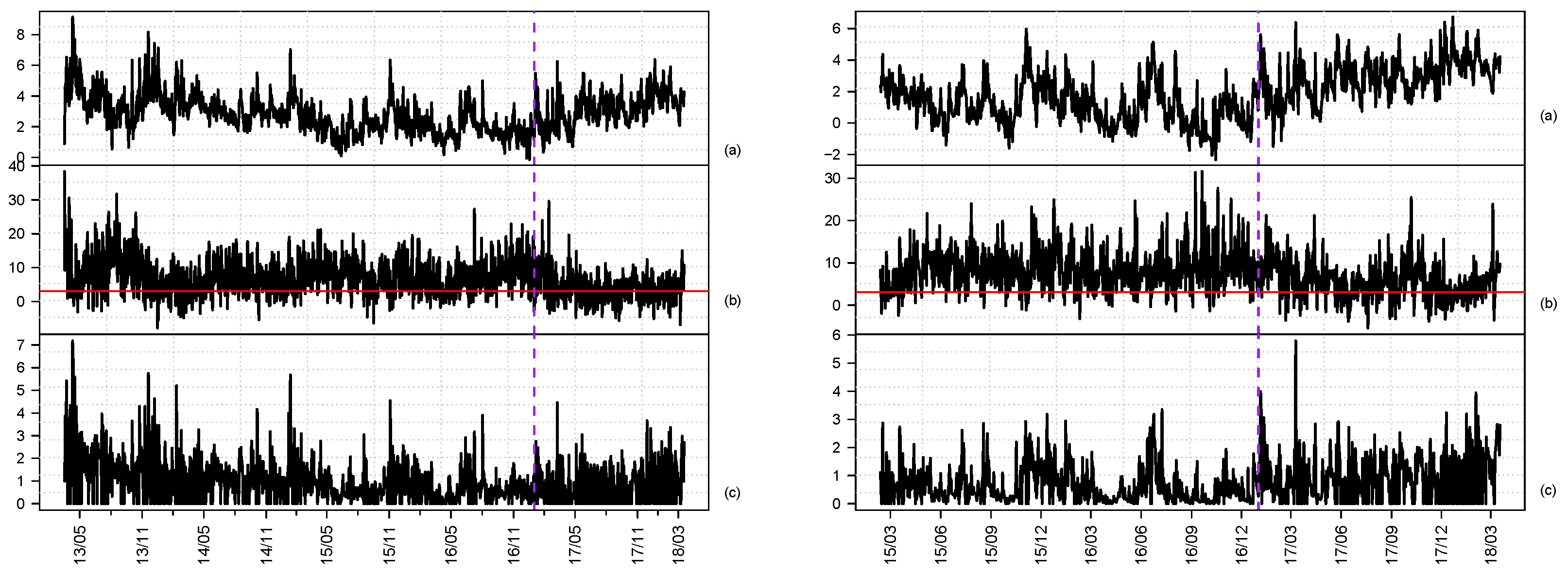
We consider the realized variance of Bitcoin from 17 March 2013 for Bitstamp and from 2 February 2015 for Coinbase up to 18 March 2018. Similar to previous results, we also consider the Hype period from 1 January 2017 to 18 March 2018. Results are also reported for the realized standard deviation, and the logarithmic realized variance, . Figure 6 displays: (i) the time series of the log realized variance; (ii) the feasible test statistics; and (iii) the significant logarithmic jump series, over the full sample for Bitstamp and Coinbase. We find that the logarithmic realized variance for the Coinbase exchange displays an increasing pattern, with the highest values in the end, and especially around December 2017 where the underline value increased significantly. Interestingly, we find that realized volatility is lower during the bubble period of 2017 compared to the bear market period of 2018.
Panel reports the test statistics from Equation (9) for . The red horizontal line indicates , i.e., the threshold after which jumps are classified as significant. Interestingly, we find a very large proportion of jumps for Bitcoin compared to the proportion usually found in other asset classes, see e.g., Andersen et al. (2007). Indeed, the proportion of jumps ranges from 27% to 92% depending on different choices of . When , the proportion of jumps over the full period is around 79% for Bitstamp and 85% for Coinbase. If we focus on the Hype period the proportion of jumps is halved for both exchanges. This results further indicates the growing trade intensity and the increased stability of the market over time.
Table 5 reports the summary statistics for the realized variance and its transformations. We find that both the median and the standard deviation of the realized variance and jump component are higher during the Hype period. We also find that similar to Andersen et al. (2001a) and Andersen et al. (2001b), we are not able to reject the null hypothesis of normality for the logarithmic realized variance according to the Jarque-Bera test statistics.
Model Estimation
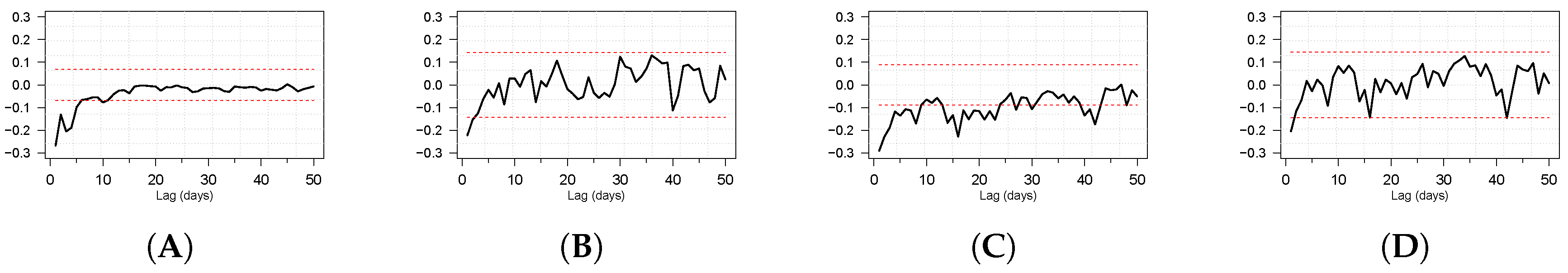
We now estimate by OLS the HAR-RV, HAR-RV-J, and HAR-RV-CJ models to the realized variance, realize standard deviation and logarithmic realized variance over the full sample for the two exchanges. Specifications that include the leverage component are also estimated and indicated with the additional label “-L”. Estimation results are reported in Table 6. Estimated coefficients are in line with those usually found in the literature for other asset classes. Interestingly, we find that specifications that include the leverage component outperform their counterpart without leverage. Regarding the estimated leverage coefficients, we see that these are negative and statistically significant at standard confidence levels. This finding is somehow in contrast with previous results by results by Catania and Grassi (2017) and Ardia et al. (2018) who document an “inverted” leverage effect for Bitcoin. To further investigate this aspect, in Figure 7 we report the empirical autocorrelation at different lags between realized variance and the leverage component, i.e., for . The plot is reported for the two exchanges for the full sample as well as for the Hype period. Results indicate that correlations are negative and statistically different from zero up to when computed over the full sample. However, when we focus on the Hype period, evidence of correlation between and is less strong. This result suggests that the leverage effect has changed over time for Bitcoin and somehow confirms the findings of Ardia et al. (2018).
4.3. Out of Sample Results
We now conduct an out of sample analysis studying the predictability of Bitcoin realized variance at different horizons. Predictions are made by the models previously introduced at horizons (one day), (one week), and (one month) using the direct method of forecast, see Marcellino et al. (2006). We start making prediction from 21 April 2014 for Bitstamp and 17 March 2016 for Coinbase and than update model parameters each time a new observation becomes available during the whole forecast periods using a fixed rolling window. The length of the out of sample is and for Bitstamp and Coinbase, respectively. Results are compared with the Random Walk (RW) specification defined by:
Let be the prediction made at time t for time . Comparison among different specification is performed according to the mean absolute forecast error (MAFE) and root mean square forecast error (RMSFE). MAFE at horizon h is defined as:
while RMSFE as:
where T is the length of the in sample period. Models with lower MAFE and RMSFE are preferred. Table 7 reports the results computed over the full sample. Results for the Hype period are similar and are available upon request to the second author.
Along with the MAFE and RMSFE measures, the table also reports the of the Mincer–Zarnowitz regression defined by:
as well as the Diebold and Mariano (1994) test statistics of each model with respect to the benchmark RW (DM1) and with respect to the plain HAR-RV model (DM2). Results indicate that predictability is higher for lower forecast horizons. Indeed, looking at the we find that when , up to of the log realized variance variability can be predicted with the HAR-RV-CJ model. However, when the decreases to only . Overall, the inclusion of jumps does not always translate in better predictions. In this respect, results are a bit mixed. Differently, models that include the leverage component seem to generally perform better than the standard HAR-RV model. Looking at the Diebold Mariano test statistic with respect to the benchmark model (DM1), we find strong evidence of predictability of all specifications. Differently, when we focus on predictability with respect to the plain HAR-RV model, results are mixed and do not show a clear pattern. Comparing results between the two exchanges indicates that realized variance is easier to predict in the Coinbase exchange.
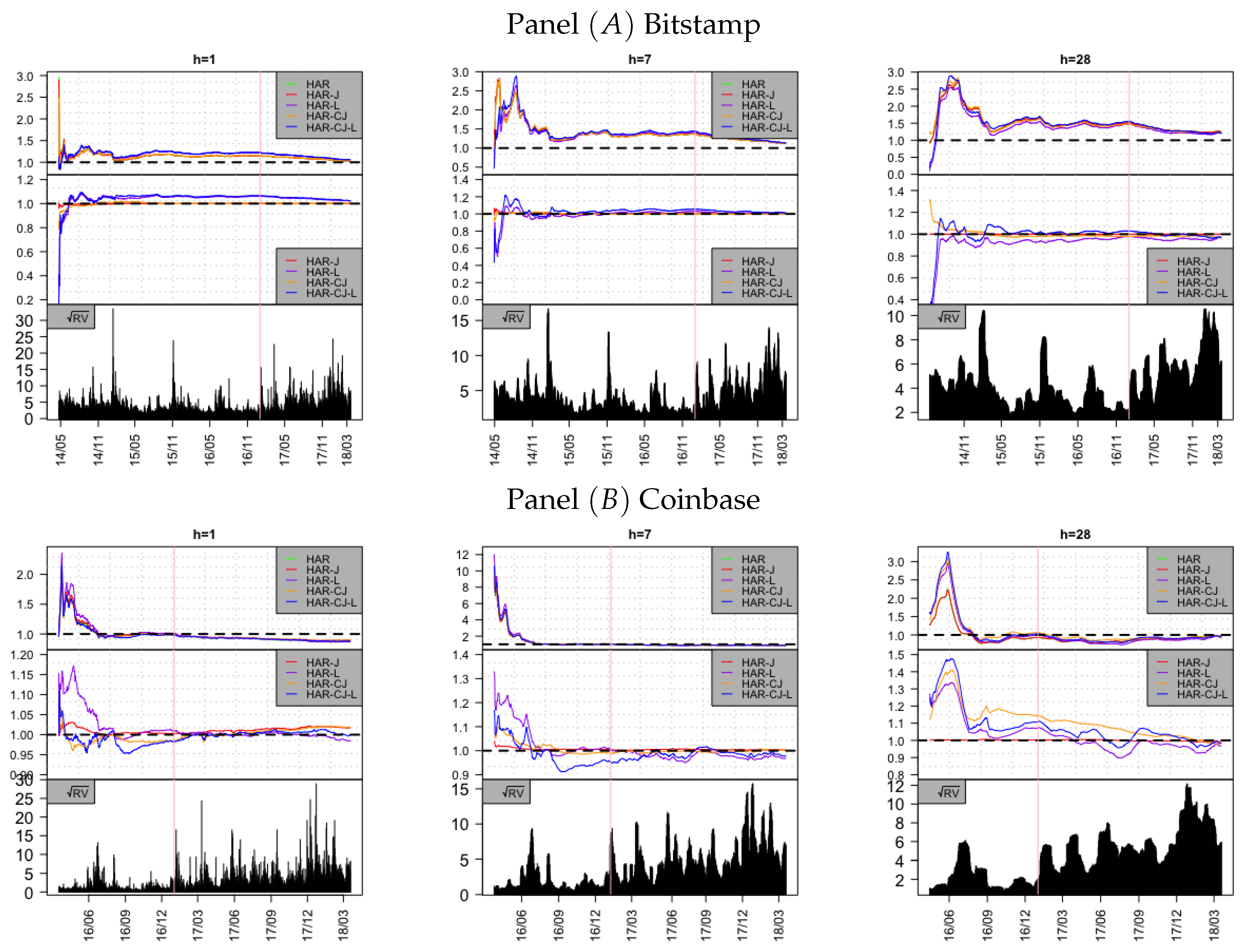
To conclude our analysis we study the stability of prediction gains with respect to the RW benchmark over time. To do so, we compute the cumulative absolute error of a forecast model over the cumulative absolute error of the benchmark model. Specifically, the ratio of cumulative absolute errors RCAE at time f is defined as:
where is the forecast error of generic model j at time s and is the forecast error of the benchmark specification. Results are reported for and . Values of below one indicate outperformance with respect to the benchmark and viceversa. Figure 8 displays the for the log realized variance for different forecast horizons and the two exchanges. In the top graph of each sub-figure the comparison is performed with respect to RW, while in the bottom graphs we use HAR-RV as the benchmark. Results are very clear and show that predictability of the realized variance is increased over time. Indeed, at the start of the sample we observe large losses of all models with respect to RW and HAR-RV probably due to uncertainty in estimated parameters. However, at the end of the forecasting period those losses seem to vanish suggesting that volatility becomes more easy to predict. Across the different specifications we observe that HAR-L and HAR-CJ-L are the top performer. This result confirms the in sample findings and indicates that the leverage component is important for volatility prediction of Bitcoin. A comparison across the two exchanges also suggests that volatility in the Coinbase exchange is easier to predict.
5. Conclusions
In this paper, we analysed Bitcoin returns sampled at high frequency and its realized variance. Raw Bitcoin transactions have been downloaded from the two exchanges Bitstamp and Coinbase. After detailing how raw data are cleaned, we started our analysis focusing on the in sample properties of Bitcoin logarithmic returns sampled at different frequencies. Results about the autocorrelation structure of Bitcoin returns as well as the intraday and intraweek seasonality of Bitcoin volatility and volumes are reported. The second part the paper focuses on predicting realized variance for Bitcoin using several forecasting models. Our results indicate that the predictability of Bitcoin realized variance is increased over time, and that predictability varies with the forecast horizon. Results extend those reported by Catania et al. (2019) and Catania et al. (2018) to the high frequency case and are consistent with previous findings reported for lower frequencies. We have also documented the presence of leverage effect for Bitcoin when realized variance is used. However, this finding is in contrast with previous results reported by Catania and Grassi (2017) and Ardia et al. (2018) where an “inverted” leverage effect is found. However, we note that differently from Catania and Grassi (2017) and Ardia et al. (2018) who use financial econometrics models to filter the conditional volatility of Bitcoin, in this study we estimate volatility using the realized variance estimator of Andersen et al. (2001a). Furthermore, our results also indicate that the leverage effect is less evident during the Hype period. Through the paper, all results have been detailed with respect to the two exchange rates as well as with a focus on the recent 2017–2018 period.
We believe that our results can be used by private investors as well as by hedge funds to improve their forecasting models for Bitcoin as well as for pricing of derivative securities. Furthermore, central banks who are considering issuing their own digital currency like Ecuador, Tunisia, and Sweden can exploits our results to improve the efficiency and reduce the volatility of the resulting market.
We have not investigated the presence of possible arbitrage opportunities across the two exchanges. Possible extensions can be made in this direction. Additionally, our results can be extended to a multivariate analysis aiming at investigating the lead/lag structure of different cryptocurrencies observed at high frequency.
Author Contributions
L.C. conceived of the presented idea. M.S. implemented the analysis under the supervision of L.C. Both authors discussed the results and contributed to the final manuscript.
Funding
This research received no external funding.
Conflicts of Interest
The authors declare no conflict of interest.
References
- Andersen, Torben G., Tim Bollerslev, Francis X. Diebold, and Heiko Ebens. 2001a. The distribution of realized stock return volatility. Journal of Financial Economics 61: 43–76. [Google Scholar] [CrossRef]
- Andersen, Torben G., Tim Bollerslev, Francis X. Diebold, and Paul Labys. 2001b. The distribution of realized exchange rate volatility. SSRN Electronic Journal 27: 42–55. [Google Scholar]
- Andersen, Torben G., Tim Bollerslev, and Francis X. Diebold. 2007. Roughing it up: Including jump components in the measurement, modeling, and forecasting of return volatility. Review of Economics and Statistics 89: 701–20. [Google Scholar] [CrossRef]
- Ardia, David, Keven Bluteau, Kris Boudt, and Leopoldo Catania. 2018. Forecasting risk with markov-switching garch models: A large-scale performance study. International Journal of Forecasting 34: 733–47. [Google Scholar] [CrossRef]
- Ardia, David, Keven Bluteau, and Maxime Rüede. 2018. Regime changes in Bitcoin GARCH volatility dynamics. Finance Research Letters. [Google Scholar] [CrossRef]
- Balcilar, Mehmet, Elie Bouri, Rangan Gupta, and David Roubaud. 2017. Can volume predict bitcoin returns and volatility? A quantiles-based approach. Economic Modelling 64: 74–81. [Google Scholar] [CrossRef]
- Bariviera, Aurelio F. 2017. The inefficiency of bitcoin revisited: A dynamic approach. Economics Letters 161: 1–4. [Google Scholar] [CrossRef]
- Barndorff-Nielsen, Ole, Peter R. Hansen, Asger Lunde, and Neil Shephard. 2009. Realized kernels in practice: trades and quotes. Econometrics Journal 12: C1–C32. [Google Scholar] [CrossRef]
- Barndorff-Nielsen, Ole E. 2004. Power and bipower variation with stochastic volatility and jumps. Journal of Financial Econometrics 2: 1–37. [Google Scholar] [CrossRef]
- Barndorff-Nielsen, Ole E., and Neil Shephard. 2003. Realized power variation and stochastic volatility models. Bernoulli 9: 243–65. [Google Scholar] [CrossRef]
- Barndorff-Nielsen, Ole E., Svend Erik Graversen, Jean Jacod, Mark Podolskij, and Neil Shephard. 2006. A central limit theorem for realised power and bipower variations of continuous semimartingales. In From Stochastic Calculus to Mathematical Finance. Berlin/Heidelberg: Springer, pp. 33–68. [Google Scholar]
- Bauwens, Luc, Christian M. Hafner, and Sébastien Laurent. 2012. Handbook of Volatility Models and Their Applications. New York: John Wiley & Sons, vol. 3. [Google Scholar]
- Black, Fischer. 1976. Studies of Stock Price Volatility Changes. In Proceedings of the 1976 Meeting of the Business and Economic Statistics Section. Washington: American Statistical Association, pp. 177–181. [Google Scholar]
- Bloomberg. 2017. Nasdaq Plans to Introduce Bitcoin Futures. Available online: https://www.bloomberg.com/news/articles/2017-11-29/nasdaq-is-said-to-plan-bitcoin-futures-joining-biggest-rivals (accessed on 10 February 2019).
- Breedon, Francis, and Angelo Ranaldo. 2013. Intraday patterns in FX returns and order flow. Journal of Money, Credit and Banking 45: 953–65. [Google Scholar] [CrossRef]
- Brownlees, Christian T., and Giampiero M. Gallo. 2006. Financial econometric analysis at ultra-high frequency: Data handling concerns. Computational Statistics & Data Analysis 51: 2232–245. [Google Scholar]
- Catania, Leopoldo, and Stefano Grassi. 2017. Modelling crypto-currencies financial time-series. SSRN Electronic Journal. [Google Scholar] [CrossRef]
- Catania, Leopoldo, Stefano Grassi, and Francesco Ravazzolo. 2019. Forecasting cryptocurrencies under model and parameter instability. International Journal of Forecasting 35: 485–501. [Google Scholar] [CrossRef]
- Catania, Leopoldo, Stefano Grassi, and Francesco Ravazzolo. 2018. Predicting the volatility of cryptocurrency time–series. In Mathematical and Statistical Methods for Actuarial Sciences and Finance: MAF 2018. Edited by Marco Corazza, María Durbán, Aurea Grané, Cira Perna and Marilena Sibillo. New York: Springer. [Google Scholar]
- CME. 2017. CME Group Announces Launch of Bitcoin Futures. Available online: http://www.cmegroup.com/media-room/press-releases/2017/10/31/cme_group_announceslaunchofbitcoinfutures.html (accessed on 10 February 2019).
- Corsi, Fulvio. 2008. A simple approximate long-memory model of realized volatility. Journal of Financial Econometrics 7: 174–96. [Google Scholar] [CrossRef]
- Corsi, Fulvio, Francesco Audrino, and Roberto Renò. 2012. HAR modeling for realized volatility forecasting. In Handbook of Volatility Models and Their Applications. Hoboken: John Wiley & Sons, Inc., pp. 363–82. [Google Scholar]
- Creal, Drew, Siem Jan Koopman, and André Lucas. 2013. Generalized Autoregressive Score Models with Applications. Journal of Applied Econometrics 28: 777–95. [Google Scholar] [CrossRef]
- Cryptocoinsnews. 2017. Tokyo Financial Exchange Plans for Bitcoin Futures Launch. Available online: https://www.cryptocoinsnews.com/breaking-tokyo-financial-exchange-plans-bitcoin-futures-launch/ (accessed on 10 February 2019).
- Dacorogna, Michael M., Ulrich A. Müller, Robert J. Nagler, Richard B. Olsen, and Olivier V. Pictet. 1993. A geographical model for the daily and weekly seasonal volatility in the foreign exchange market. Journal of International Money and Finance 12: 413–38. [Google Scholar] [CrossRef]
- Diebold, Francis, and Robert Mariano. 1994. Comparing Predictive Accuracy. Journal of Business and Economic Statistics 13: 253–65. [Google Scholar]
- Dyhrberg, Anne H. 2016. Bitcoin, gold and the dollar—A GARCH volatility analysis. Finance Research Letters 16: 85–92. [Google Scholar] [CrossRef]
- Gencay, Ramazan, Michel Dacorogna, Ulrich A. Muller, Richard Olsen, and Olivier Pictet. 2001. An Introduction to High-Frequency Finance. Amsterdam: Elsevier Science Publishing Co. Inc. [Google Scholar]
- Hansen, Peter R., and Asger Lunde. 2005. A forecast comparison of volatility models: Does anything beat a garch (1, 1)? Journal of Applied Econometrics 20: 873–89. [Google Scholar] [CrossRef]
- Harvey, Andrew C. 2013. Dynamic Models for Volatility and Heavy Tails: With Applications to Financial and Economic Time Series. Cambridge: Cambridge University Press, Vol. 52. [Google Scholar]
- Katsiampa, Paraskevi. 2017. Volatility estimation for bitcoin: A comparison of GARCH models. Economics Letters 158: 3–6. [Google Scholar] [CrossRef]
- Liu, Lily, Andrew Patton, and Kevin Sheppard. 2015. Does anything beat 5-minute rv? A comparison of realized measures across multiple asset classes. Journal of Econometrics 187: 293–311. [Google Scholar] [CrossRef]
- Marcellino, Massimiliano, James H. Stock, and Mark W. Watson. 2006. A comparison of direct and iterated multistep ar methods for forecasting macroeconomic time series. Journal of econometrics 135: 499–526. [Google Scholar] [CrossRef]
- Nakamoto, Satoshi. 2009. Bitcoin: A Peer-to-Peer Electronic Cash System. Available online: https://bitcoin.org/bitcoin.pdf (accessed on 10 February 2019).
- Nelson, Daniel B. 1991. Conditional heteroskedasticity in asset returns: A new approach. Econometrica: Journal of the Econometric Society 59: 347–70. [Google Scholar] [CrossRef]
- Phillip, Andrew, Jennifer S. K. Chan, and Shelton Peiris. 2018. A new look at cryptocurrencies. Economics Letters 163: 6–9. [Google Scholar] [CrossRef]
- Stavroyiannis, Stavros. 2018. Value-at-risk and related measures for the bitcoin. The Journal of Risk Finance 19: 127–136. [Google Scholar] [CrossRef]
- Taylor, Stephen J., and Xinzhong Xu. 1997. The incremental volatility information in one million foreign exchange quotations. Journal of Empirical Finance 4: 317–40. [Google Scholar] [CrossRef]
- Zakoian, Jean-Michel. 1994. Threshold Heteroskedastic Models. Journal of Economic Dynamics and Control 18: 931–55. [Google Scholar] [CrossRef]
- Zhang, Yuanyuan, Stephen Chan, Jeffrey Chu, and Saralees Nadarajah. 2019. Stylised facts for high frequency cryptocurrency data. Physica A: Statistical Mechanics and Its Applications 513: 598–612. [Google Scholar] [CrossRef]
| 1. | Specifically, 54.42% for the Bitstamp exchange and 68.78% for the Coinbase exchange. |
| 2. | Among several exchanges where Bitcoin is traded we have selected two of the most active ones. Another possibility would have been to consider GDAX instead of Coinbase since this exchange might give a better representation of Bitcoin. However, we have decided to use Coinbase since, differently from GDAX and Bitstamp which are traditional exchanges, it is a click and buy exchange which allows investor to immediately invest in Bitcoin. We thank an anonymous referee for pointing out this to us. |
| 3. | See also Balcilar et al. (2017) who examine the causal relation between Bitcoin return/volatility and traded volumes. |
| 4. | However, we acknowledge that at the time of writing there is a lag of 10.83 min between the placement and execution of a trade on Bitstamp. Differently, on Coinbase trade execution is immediate. |
| 5. | Please note that Bitcoin is traded 7 days a week. |
Figure 1.
Gaussian kernel densities estimated using 5 min returns over the daily mean (a); standard deviation (b); skewness (c) and excess of kurtosis (d) coefficients for Bitstamp (panel A) and Coinbase (panel B). Results are reported for the full sample (black) and for the Hype period (red).
Figure 1.
Gaussian kernel densities estimated using 5 min returns over the daily mean (a); standard deviation (b); skewness (c) and excess of kurtosis (d) coefficients for Bitstamp (panel A) and Coinbase (panel B). Results are reported for the full sample (black) and for the Hype period (red).

Figure 2.
Linear correlation coefficient calculated as a function of the size of the time interval of returns for Bitstamp left and Coinbase right. The horizontal axis is the logarithmic of the time interval.
Figure 2.
Linear correlation coefficient calculated as a function of the size of the time interval of returns for Bitstamp left and Coinbase right. The horizontal axis is the logarithmic of the time interval.

Figure 3.
First order serial autocorrelation coefficient estimated using a fixed rolling windows of one month for Bitstamp (top figures) and Coinbase (bottom figures). Horizontal dashed lines indicate the 95% confidence interval. The dashed vertical line indicates the start of the Hype period at the begin of January 2017. Results are reported for Bitcoin logarithmic returns sampled at 5, 15, 30, and 60 min.

Figure 4.
Intraday realized volatility (red lines, left axis) and average volumes (vertical bars, right axis) computed every 30 min for Bitcoin traded at the Bitstamp (panel A) and Coinbase (panel B) exchanges.
Figure 4.
Intraday realized volatility (red lines, left axis) and average volumes (vertical bars, right axis) computed every 30 min for Bitcoin traded at the Bitstamp (panel A) and Coinbase (panel B) exchanges.

Figure 5.
Weekly seasonality computed for the Bitstamp (left figures) and Coinbase (right figures) exchanges over the full sample and Hype period. Red lines report the average realized volatility (left axis) while the vertical bars report the average sum of volume (right axis).
Figure 5.
Weekly seasonality computed for the Bitstamp (left figures) and Coinbase (right figures) exchanges over the full sample and Hype period. Red lines report the average realized volatility (left axis) while the vertical bars report the average sum of volume (right axis).

Figure 6.
Plot of logarithmic realized variance (a), (b) and logarithmic significant jumps (c) over time. Purple vertical dashed lines indicate the start of the Hype period. The horizontal red line indicates the quantile of a standard Gaussian distribution for . Figures on the left panel are for Bitstamp, figures on the right panel for Coinbase.

Figure 7.
Empirical cross correlation at different lags between realized variance and the leverage component, for . Panels (A) and (B) report results for Bitstamp over the full sample and the Hype period, respectively. Panels (C) and (D) report results for Coinbase over the full sample and the Hype period, respectively. Horizontal red dashed lines indicate 95% confidence bounds.

Figure 8.
Relative cumulative absolute errors of several forecasting models with respect to RW (first sub-figure) and HAR-RV (second sub-figure). The third sub-figure reports the evolution of the realized standard deviation over time. The red vertical lines correspond to the start of the Hype period. Results are reported for Bitstamp in panel (A) and for Coinbase in panel (B) for the three forecast horizons , , and .


Table 1.
Number of outliers and average number of outliers per day in percentage points as a function of the rolling trimmed mean parameter k and the granularity parameter . Results are reported for Coinbase and Bitstamp using Equation (1) with .
Table 1.
Number of outliers and average number of outliers per day in percentage points as a function of the rolling trimmed mean parameter k and the granularity parameter . Results are reported for Coinbase and Bitstamp using Equation (1) with .
| Bitstamp | |||||||||
| Number of outliers | 141,029 | 134,584 | 128,934 | 104,018 | 99,007 | 85,593 | 82,623 | 78,603 | 75,438 |
| Average outliers per day | 0.51% | 0.46% | 0.42% | 0.38% | 0.34% | 0.30% | 0.31% | 0.27% | 0.25% |
| Coinbase | |||||||||
| Number of outliers | 118,162 | 107,936 | 100,570 | 98,037 | 89,922 | 84,009 | 85,499 | 78,482 | 73,521 |
| Average outliers per day | 0.24% | 0.20% | 0.17% | 0.19% | 0.16% | 0.14% | 0.17% | 0.14% | 0.12% |
Table 2.
This table summarizes the results from the cleaning procedure. Starting from the raw dataset, transactions associated with non positive volume are removed. Outliers are identified following the procedure of Brownlees and Gallo (2006). The “Simultaneous ticks” reports the number of transactions that occurs within the same second. The row “Final sample size in seconds” and “ Trading days” report the number of equally spaced observations in second and the number of trading days, respectively. Results are reported for the two exchanges Bitstamp and Coinbase as well as for the full sample and the sub–sample “Hype”.
| Bitstamp | Coinbase | |||
|---|---|---|---|---|
| Full Sample | Hype | Full Sample | Hype | |
| Raw observations | 22,346,195 | 12,217,195 | 39,285,138 | 27,126,897 |
| Volume | 1112 | 98 | 0 | 0 |
| Outliers | 104,295 | 61,350 | 103,071 | 85,418 |
| Simultaneous ticks | 9,976,748 | 5,338,296 | 28,400,400 | 18,861,682 |
| Final sample size in seconds | 12,263,584 | 6,817,445 | 10,781,667 | 8,179,797 |
| Trading days | 1825 | 442 | 1132 | 442 |
Table 3.
Comparison over the period 2015–2018 between daily average realized variance of Bitcoin, measured using Coinbase and Bitstamp 5-min returns and S&P 500 measured using the volatility index VIX. The first four columns report the sample while the last four columns the standard deviation (i.e., the volatility of volatility).
| Mean | Standard Deviation | |||||||
|---|---|---|---|---|---|---|---|---|
| 2015 | 2016 | 2017 | 2018 | 2015 | 2016 | 2017 | 2018 | |
| S&P 500 | 16.67 | 15.83 | 11.09 | 16.64 | 4.34 | 3.97 | 1.36 | 5.09 |
| Coinbase | 11.25 | 6.89 | 37.24 | 59.02 | 29.76 | 17.26 | 78.46 | 67.15 |
| Bitstamp | 23.10 | 10.08 | 37.46 | 64.88 | 72.48 | 14.69 | 57.19 | 62.44 |
Table 4.
Summary statistics of the 5 min Bitcoin log returns. Results are reported for the two exchanges Bitstamp and Coinbase over the full period “Full” and conditional on the Hype period.
Table 4.
Summary statistics of the 5 min Bitcoin log returns. Results are reported for the two exchanges Bitstamp and Coinbase over the full period “Full” and conditional on the Hype period.
| Bitstamp | Coinbase | |||
|---|---|---|---|---|
| Full | Hype | Full | Hype | |
| Maximum | 61.09 | 7.41 | 10.62 | 10.62 |
| Minimum | −36.89 | −15.54 | −21.02 | −21.02 |
| Mean | 0.00 | 0.00 | 0.00 | 0.00 |
| Median | 0.00 | 0.00 | 0.00 | 0.00 |
| Std. Dev. | 0.31 | 0.33 | 0.20 | 0.31 |
| Skewness | −0.28 | −0.38 | −0.58 | −0.40 |
| Excess of kurtosis | 8.84 | 8.28 | 14.36 | 10.22 |
Table 5.
Summary statistic for the realized variance, realized standard deviation and logarithmic realized variance. Panel (A) reports results for the full sample while panel (B) for the Hype period. The rwo J.test reports the Jarque-Bera test statistics for the null hypothesis of Gaussianity.
Panel (A)—Full sample
| Bitstamp | Coinbase | |||||||||||
|---|---|---|---|---|---|---|---|---|---|---|---|---|
| Maximum | 9374.99 | 96.82 | 9.15 | 1320.43 | 36.34 | 7.19 | 835.73 | 28.91 | 6.73 | 326.73 | 18.08 | 5.79 |
| Minimum | 0.87 | 0.93 | −0.14 | 0.12 | 0.35 | 0.12 | 0.01 | 0.31 | −2.31 | 0.02 | 0.15 | 0.02 |
| Mean | 54.94 | 5.23 | 2.86 | 7.35 | 1.85 | 1.29 | 21.47 | 3.41 | 1.82 | 2.69 | 1.25 | 0.88 |
| Median | 15.63 | 3.95 | 2.75 | 2.01 | 1.42 | 1.10 | 5.81 | 2.41 | 1.76 | 1.02 | 1.00 | 0.70 |
| Std. Dev. | 311.15 | 5.26 | 1.23 | 45.42 | 1.98 | 0.87 | 53.93 | 3.14 | 1.57 | 11.48 | 1.06 | 0.73 |
| Skewness | 21.19 | 7.39 | 0.69 | 21.16 | 7.96 | 1.82 | 7.51 | 2.72 | 0.19 | 24.81 | 5.51 | 1.34 |
| Kurtosis | 541.82 | 94.59 | 4.11 | 552.17 | 102.12 | 8.60 | 81.77 | 14.48 | 2.55 | 694.19 | 74.09 | 5.77 |
| J.test | 239 | 7612 | ||||||||||
Panel (B)—Hype period
| Bitstamp | Coinbase | |||||||||||
|---|---|---|---|---|---|---|---|---|---|---|---|---|
| Maximum | 588.38 | 24.26 | 6.38 | 37.84 | 6.15 | 3.66 | 835.73 | 28.91 | 6.73 | 326.73 | 18.08 | 5.79 |
| Minimum | 1.40 | 1.19 | 0.34 | 0.26 | 0.51 | 0.23 | 0.23 | 0.48 | −1.48 | 0.07 | 0.26 | 0.06 |
| Mean | 42.23 | 5.64 | 3.18 | 4.62 | 1.91 | 1.44 | 41.04 | 5.21 | 2.89 | 5.16 | 1.78 | 1.30 |
| Median | 24.56 | 4.96 | 3.20 | 2.90 | 1.70 | 1.36 | 18.70 | 4.32 | 2.93 | 2.19 | 1.48 | 1.16 |
| Std. Dev. | 58.99 | 3.23 | 1.06 | 5.37 | 0.99 | 0.72 | 76.98 | 3.73 | 1.29 | 21.39 | 1.42 | 0.76 |
| Skewness | 4.44 | 1.80 | 0.06 | 3.10 | 1.32 | 0.53 | 5.49 | 2.30 | −0.06 | 14.05 | 6.77 | 1.41 |
| Kurtosis | 31.60 | 8.08 | 2.86 | 16.08 | 5.49 | 2.90 | 43.11 | 10.97 | 3.16 | 210.54 | 73.42 | 7.91 |
| J. test | 714 | 31,853 | 1562 | |||||||||
Table 6.
OLS in sample estimated coefficients for the five different HAR models for Bitstamp (panel A) and Coinbase (panel B). HAC standard errors are reported in parentheses based on the Newey-West correction. The apexes a–d report the significance level, , , and .
Panel (A)—Bitstamp
| HAR-RV | HAR-RV-J | HAR-RV-L | HAR-RV-CJ | HAR-RV-CJ-L | |||||||||||
|---|---|---|---|---|---|---|---|---|---|---|---|---|---|---|---|
| c | |||||||||||||||
| adj. | |||||||||||||||
Panel (B)—Coinbase
| HAR-RV | HAR-RV-J | HAR-RV-L | HAR-RV-CJ | HAR-RV-CJ-L | |||||||||||
|---|---|---|---|---|---|---|---|---|---|---|---|---|---|---|---|
| c | |||||||||||||||
| 26% | |||||||||||||||
| adj. | 26% | ||||||||||||||
Table 7.
This table reports the out of sample forecast results for different HAR models. Results for Bitstamp are reported in panel (A) for Coinbase in panel (B) for the three forecast horizons , , and . Diebold Mariano test statistics with respect to the RW model (DM1) and HAR-RV model (DM2) are reported. p-values based on the asymptotic Gaussian distribution with HAC standard errors are reported in parenthesis.
Panel (A)—Bitstamp
| Daily | |||||||||||||||||||||||
|---|---|---|---|---|---|---|---|---|---|---|---|---|---|---|---|---|---|---|---|---|---|---|---|
| Model | RW | HAR-RV | HAR-RV-J | HAR-RV-L | HAR-RV-CJ | HAR-RV-CJ-L | |||||||||||||||||
| MAFE | |||||||||||||||||||||||
| RMSFE | |||||||||||||||||||||||
| Weekly | |||||||||||||||||||||||
| Model | RW | HAR-RV | HAR-RV-J | HAR-RV-L | HAR-RV-CJ | HAR-RV-CJ-L | |||||||||||||||||
| MAFE | |||||||||||||||||||||||
| RMSFE | 072 | ||||||||||||||||||||||
| Monthly | |||||||||||||||||||||||
| Model | RW | HAR-RV | HAR-RV-J | HAR-RV-L | HAR-RV-CJ | HAR-RV-CJ-L | |||||||||||||||||
| MAFE | |||||||||||||||||||||||
| RMSFE | |||||||||||||||||||||||
Panel (B)—Coinbase
| Daily | |||||||||||||||||||||||
|---|---|---|---|---|---|---|---|---|---|---|---|---|---|---|---|---|---|---|---|---|---|---|---|
| Model | RW | HAR-RV | HAR-RV-J | HAR-RV-L | HAR-RV-CJ | HAR-RV-CJ-L | |||||||||||||||||
| MAFE | |||||||||||||||||||||||
| RMSFE | |||||||||||||||||||||||
| Weekly | |||||||||||||||||||||||
| Model | RW | HAR-RV | HAR-RV-J | HAR-RV-L | HAR-RV-CJ | HAR-RV-CJ-L | |||||||||||||||||
| MAFE | |||||||||||||||||||||||
| RMSFE | |||||||||||||||||||||||
| Monthly | |||||||||||||||||||||||
| Model | RW | HAR-RV | HAR-RV-J | HAR-RV-L | HAR-RV-CJ | HAR-RV-CJ-L | |||||||||||||||||
| MAFE | |||||||||||||||||||||||
| RMSFE | |||||||||||||||||||||||
© 2019 by the authors. Licensee MDPI, Basel, Switzerland. This article is an open access article distributed under the terms and conditions of the Creative Commons Attribution (CC BY) license (http://creativecommons.org/licenses/by/4.0/).
Share and Cite
MDPI and ACS Style
Catania, L.; Sandholdt, M. Bitcoin at High Frequency. J. Risk Financial Manag. 2019, 12, 36. https://doi.org/10.3390/jrfm12010036
AMA Style
Catania L, Sandholdt M. Bitcoin at High Frequency. Journal of Risk and Financial Management. 2019; 12(1):36. https://doi.org/10.3390/jrfm12010036
Chicago/Turabian StyleCatania, Leopoldo, and Mads Sandholdt. 2019. "Bitcoin at High Frequency" Journal of Risk and Financial Management 12, no. 1: 36. https://doi.org/10.3390/jrfm12010036