Does Oil Price Drive World Food Prices? Evidence from Linear and Nonlinear ARDL Modeling


1
Department of Economics, Northern Border University, 91431 Arar, Saudi Arabia
2
Department of Economics and Quantitative Methods, University of Tunis, 1007 Tunis, Tunisia
3
Department of Economics, University of Sousse, 4054 Sousse, Tunisia
*
Author to whom correspondence should be addressed.
Economies 2019, 7(1), 12; https://doi.org/10.3390/economies7010012
Submission received: 29 November 2018
/
Revised: 14 January 2019
/
Accepted: 19 January 2019
/
Published: 12 February 2019
Abstract
:The macroeconomic outcomes of oil price fluctuations have been at the forefront of the debate among economists, financial analysts and policymakers over the last decades. Among others, the oil price–food price nexus has particularly received a great deal of attention. While an abundant body of literature has focused on the linear relationship between oil price and food price, little is known regarding the nonlinear interactions between them. The aim of this paper is to conduct aggregated and disaggregated analyses of the impact of the Brent and West Texas Intermediate (WTI) oil prices on international food prices between January 1990 and October 2017. The empirical investigation is based on the estimation of linear and nonlinear autoregressive distributed lag (ARDL) models. The findings confirm the presence of asymmetries since the overall food price is only affected by positive shocks on oil price in the long-run. While the dairy price index reacts to both positive and negative changes of oil price, the impact of oil price increases is found to be greater. Finally, the asymmetry is present for some other agricultural commodity prices in the short-run, since they respond only to oil price decreases. All in all, the study concludes that studies assuming the presence of a symmetric impact of oil price on food price might be flawed. The findings are important for the undertaking of future studies and the design of international and national policies in the fight against food insecurity.
1. Introduction
Over the last decades, the international community has faced many challenges regarding food security, perhaps the most prominent of which is the sharp upturn of prices. According to the Food and Agriculture Organization of the United Nations (hereafter FAO), the international prices of essential foods reached their highest levels for 30 years in June 2008 (FAO 2009). The overall food price index climbed by 27% in 2007 and 25% in 2008. A sharp rise of specific agricultural commodity prices has been also observed during the same period. For instance, the price indices of dairy, vegetable oils and cereals increased by 69%, 52% and 37% in 2007, respectively. Consequently, the FAO (2009) estimates suggest that 115 million additional people were pushed into chronic hunger during the 2007–2008 price boom. More recent data suggest that about 124 million people across 51 countries faced food insecurity in 2017 (Food Security Information Network 2018). In February 2011, the FAO Food Price Index surpassed the peak attained in June 2008 by reaching a historical level of 240.1%, and then remained stable before starting to fall from April 2014.The global food crisis that has occurred over the last decade has sparked the interest of researchers and has been the subject of active academic and political debate, given the disastrous impact of rising prices on people’s well-being in both developed and developing countries. Indeed, higher agricultural products prices might exert a substantial impact on socioeconomic stability by affecting the producers’ income, the consumer purchasing power, the balance of payments and the government budget.
The high variability of global agricultural commodity prices observed during the 2000s has revived the debate on the main drivers of agricultural commodity prices’ instability. Several studies have been carried out and have focused particularly on the agricultural commodity market price formation by providing several potential explanations. The body of theoretical and empirical literature dealing with this issue shows that the excessive variability of agricultural commodity prices is a dynamic process resulting from many interrelated factors. For instance, Schmidhuber and Tubiello (2007) and Wheeler and von Braun (2013) point out that food price variability is partially affected by climate change. Some other authors have rather examined the relationship between agricultural price variability and a set of macroeconomic variables such as money supply (Barnett et al. 1983; Asfaha and Jooste 2007), per capita income (Apergis and Rezitis 2011; Wong and Shamsudin 2017) and the real exchange rate (Harri et al. 2009; Nazlioglu and Soytas 2011). Recently, special attention has been paid to the speculation in commodity future markets as a potential explanation of the increasing food price variability. This phenomenon is known as the financialization of agricultural commodity markets and is based on the idea that institutional investors might play a significant role in the price boom by feeding speculative transactions. Empirically, the analysis of this issue was conducted through the study of the impact of futures prices on spot prices (Büyükşahin and Harris 2011; Lagi et al. 2015). However, Abbott et al. (2008, 2009) reduce the number of factors explaining the dynamics of agricultural commodities price to only three, namely excess demand, the value of the US dollar and the energy price. Regarding this point, relatively recent studies highlight that the energy price is considered to be a key variable that explains the dynamics of agricultural commodity prices around the world (Saghaian 2010; Fowowe 2016; Pal and Mitra 2017).
The current paper is part of this ongoing research topic and conducts an empirical study on the impact of oil price on food price at the global scale. In fact, the upward trend of oil and food prices observed during the 2000s has revived the interest of scholars in the potential relationship between them. Thus, we aim to examine empirically if and how the world food price index and the price indices of five main agricultural commodities (sugar, vegetable oils, cereals, dairy, and meat) respond to oil prices between January 1990 and October 2017. It is useful to mention that the majority of existing empirical studies implicitly maintain the assumption of a symmetric impact of oil price on food price (to cite a few, Chen et al. 2010; Nazlioglu and Soytas 2011). Such an assumption means that the impact of oil price (in absolute value) on food price is the same whether there is an increase or a decrease of oil price. Nevertheless, it is important to highlight that some authors have placed considerable attention on the study of asymmetry and nonlinearity in macroeconomic and financial relationships (Mills 1991; Narayan and Narayan 2007; Sek 2017). The asymmetric impact of oil price on the macroeconomy has been long debated and confirmed in the literature (Tatom 1988; Hamilton 1988). For instance, Hamilton (1996) concludes that oil price increases are more important than oil price decreases. There are a number of factors inducing the presence of potential asymmetric and nonlinear price adjustments. Scherer and Ross (1990) shed light on market power as a potential source of asymmetries. Moreover, Abdulai (2000) points out that the presence of imperfect competition and the inventory behavior of traders may induce asymmetric price transmissions. Finally, the fluctuation of input costs and policy changes in commodity markets are considered to be other potential sources of asymmetry (Rapsomanikis et al. 2003). Deaton and Laroque (1992) and Salisu et al. (2017) stress the asymmetric behavior of agricultural prices and highlight that these prices generally follow cycles which generally include long periods of stability followed by sudden sharp increases in the form of peaks. Accordingly, it seems to be crucial to check the presence of short- and long-run nonlinearities, and if confirmed, to estimate the asymmetric response of food price to oil price.
We propose, therefore, an empirical methodology based on the use of the linear autoregressive distributed lag (ARDL) model developed by Pesaran et al. (2001) and the nonlinear autoregressive distributed lag modeling proposed by Shin et al. (2014) to examine the oil price–food price nexus. The study adds to the existing literature in two ways. The first contribution of this paper is to decompose changes in oil price into their partial sum of positive and negative changes to investigate whether these changes have asymmetric effects on food prices. Compared to the linear version of the ARDL approach, the nonlinear ARDL approach allows the separate estimation of the impact of oil price increases and oil price decreases on the evolution of food prices. This is a crucial issue since the linear ARDL model implicitly assumes that the impact of oil price on food price is symmetric, which is unrealistic. Contrarily, the nonlinear ARDL relaxes this assumption since coefficients on oil price increases and oil price decreases are assumed to be significantly different from each other, suggesting that the impacts of oil price increases and oil price decreases are asymmetric. It would be thus naïve to use only a linear-based model to examine the oil price–food price nexus. Second, the current paper empirically examines the linear and nonlinear effects of oil price on both global and specific food prices at the global level. In fact, while a large number of studies have examined the oil price–food price relationship, none of them have considered the three issues (nonlinearity, disaggregated analysis, global analysis) at the same time. For instance, Pala (2013); Pal and Mitra (2017, 2018) and Tiwari et al. (2018) investigate the impact of oil price on different food prices around the world without giving special attention to asymmetry and nonlinearity. On the other hand, Ibrahim (2015) and Wong and Shamsudin (2017) use nonlinear ARDL modeling to examine the oil price–food price linkage in a specific country (Malaysia) and not at the global level. Finally, it is worth noting that we conduct both aggregated and disaggregated empirical analyses. In fact, the FAO global food price index is an aggregation of many price sub-indices. Such an aggregation could cloud the impact of oil price on the global food price. The disaggregated analysis is motivated by the potential presence of the Simpson Paradox1, indicating that the neutral impact of oil price on food price may be due to the aggregation of data. Considering the sub-indices might offer a clearer picture of the aforementioned relationship.
This paper is structured as follows. Section 2 outlines the related theoretical and empirical literature. In Section 3 and Section 4, the data and the empirical methodology are described. The analysis of the empirical findings is presented in Section 5. Finally, Section 6 and Section 7, respectively, provide some managerial implications and the conclusion.
2. Literature Review
On the theoretical level, several mechanisms can be invoked to explain the impact of oil price on agricultural commodities prices. According to Reboredo (2012), oil price might affect agricultural commodities prices for two reasons. First, the agricultural production consumes large quantities of energy. Such consumption occurs directly through energy products or indirectly through the use of energy-intensive inputs such as fertilizers. The second argument is based on the fact that the energy and agriculture markets have become related since 2006, due to the increased demand for soybean and corn biofuels. Furthermore, Claudio et al. (2010) examine the relationship between the oil price and agricultural commodity prices by focusing especially on the transport cost channel. The authors propose a model suggesting that the increase of fuel price leads to an increase in the cost of cereal transportation activities.
From the empirical point of view, studies focusing on the impact of oil price on agricultural commodity prices have implemented several standard methodologies and relatively sophisticated ones. A first set of studies has investigated the relationship between oil price and food price based on vector autoregressive models (VAR), cointegration and causality. In this context, Baumeister and Kilian (2014) examined the impact of oil prices on food prices by taking into account the change in U.S. biofuel policies in 2006. The authors conclude that oil price affects agricultural commodity prices, but not retail food prices, since agricultural commodities represent a small cost share of food prices. Campiche et al. (2007) implement the Johansen (1988, 1991) cointegration analysis between crude oil price and corn, soybeans, soybean oil, palm oil, and sugar prices based on weekly data covering the period 2003–2007. Although the authors found no long-run relationships during the period 2003–2005, only corn prices and soybean prices were found to be cointegrated with oil price in 2006 and 2007. Consequently, the authors conclude that the interrelationship between corn and soybean prices and oil price has been observed during the global food crisis. Saghaian (2010) performed the Johansen cointegration test for corn, soybean, wheat, crude oil and ethanol prices. The results showed that even if there is a strong correlation between oil price and agricultural commodity prices, there is little evidence of a causal impact of oil price on agricultural commodity prices.
Some authors have focused more on explaining the asymmetric response of agricultural commodity prices to oil price changes. Balcombe and Rapsomanikis (2008) investigated the presence of nonlinear long-run equilibrium adjustments between crude oil, ethanol and sugar prices in Brazil using Bayesian Monte Carlo Markov Chain algorithms. The authors concluded that there is a long-run relationship between each pair of prices and confirmed the presence of nonlinear response of sugar and ethanol prices to oil price fluctuation. Nazlioglu (2011) conducted a study focusing on the causal relationship between oil price and three main commodity prices, namely maize, soybean and wheat. The Toda and Yamamoto (1995) linear causality procedure and Diks and Panchenko (2006) nonlinear causality tests were applied to weekly data between 1994 and 2010. The linear causality analysis indicated that oil price and agricultural commodities prices do not influence each other. In contrast, the findings suggested the existence of non-linear causality ranging from oil prices to corn and soybean prices. Fowowe (2016) investigated the effects of oil price on agricultural prices in South Africa from 2 January 2003 to 31 January 2014. The author considered the prices of three agricultural products, namely maize, sunflower and soybeans, while the Brent crude oil price was used to represent the world oil price. The use of the Gregory and Hansen (1996) structural breaks cointegration test as well as the Diks and Panchenko (2006) nonlinear causality test did not support any evidence of a significant relationship between oil price and agricultural commodity prices. Ibrahim (2015) focused on the relationship between oil price and food prices in Malaysia using the nonlinear ARDL model developed by Shin et al. (2014). The author concluded the presence of a significant relationship between oil price increase and food price in both the short and long-run. The results also suggested that food price does not react to the reduction of oil prices. Overall, the study supported the presence of an asymmetric impact of oil price on food price in the Malaysian economy. Coronado et al. (2018) studied the impact of oil price on three agricultural commodity prices, namely corn, soybeans, and sugar, using linear and nonlinear causality during the period 1990–2016. While there is no evidence of linear Granger causality, the analysis reveals bidirectional nonlinear causality. Paris (2018) examined the impact of oil price on agricultural commodity prices based on daily data. The estimation of nonlinear and regime-switching models reveals the presence of long-run effects of oil price on agricultural commodity prices. Another interesting finding is that biofuel production amplifies the impact of oil price on agricultural commodity prices.
Another part of the literature has rather examined the potential effects of oil price on food price using time-varying regressions such as copula and wavelets. Reboredo (2012) assessed the interdependence between food and energy markets based on weekly data from 9 January 1998 to 15 April 2011. Three food prices (corn, soybeans and wheat) and the Brent oil price were used in the empirical analysis. The use of the copula approach reveals a weak dependence between food prices and oil price. Recently, Koirala et al. (2015) implemented the copula approach to study the dependence between commodity futures prices and energy futures prices using U.S. daily data. The authors considered five energy products (natural gas, crude oil, gasoline, diesel and biodiesel) and three agricultural commodities (corn, soybean and cattle). The findings suggested the presence of a positive correlation between agricultural commodities and energy prices. This study particularly concluded the presence of asymmetric effects, as a rise of energy prices would increase the price of agricultural commodities. The increase of energy prices leads to higher production costs, which explains the rise of agricultural commodities prices. Pal and Mitra (2017) investigated the relationship between crude oil price and the global food price index and its subcategories (dairy, cereals, vegetable oils, meat and sugar) using the wavelet approach. The study was based on monthly data ranging from January 1990 to February 2016. The wavelet approach showed that the world food prices of the different considered agricultural commodities and the Brent crude oil price co-move together, especially between mid-2001 and 2012Q3. Regarding the different agricultural commodities, the analysis revealed that the cereal price and the crude oil price were correlated between 2003 and 2012, while the dairy price was strongly correlated with the crude oil price during 2004. Finally, the analysis also suggested the existence of a correlation between oil prices and the prices of vegetable oils and sugar. Tiwari et al. (2018) examined the potential presence of co-movements between oil price and 21 agricultural commodity prices based on wavelets. The authors concluded the presence of a high degree of long-run co-movements between oil price on the one hand and wheat, maize, rice, rubber, coal, cotton, and fishmeal on the other hand. Another important finding is that the degree of co-movement intensified during the financial crisis.
3. Data Issues
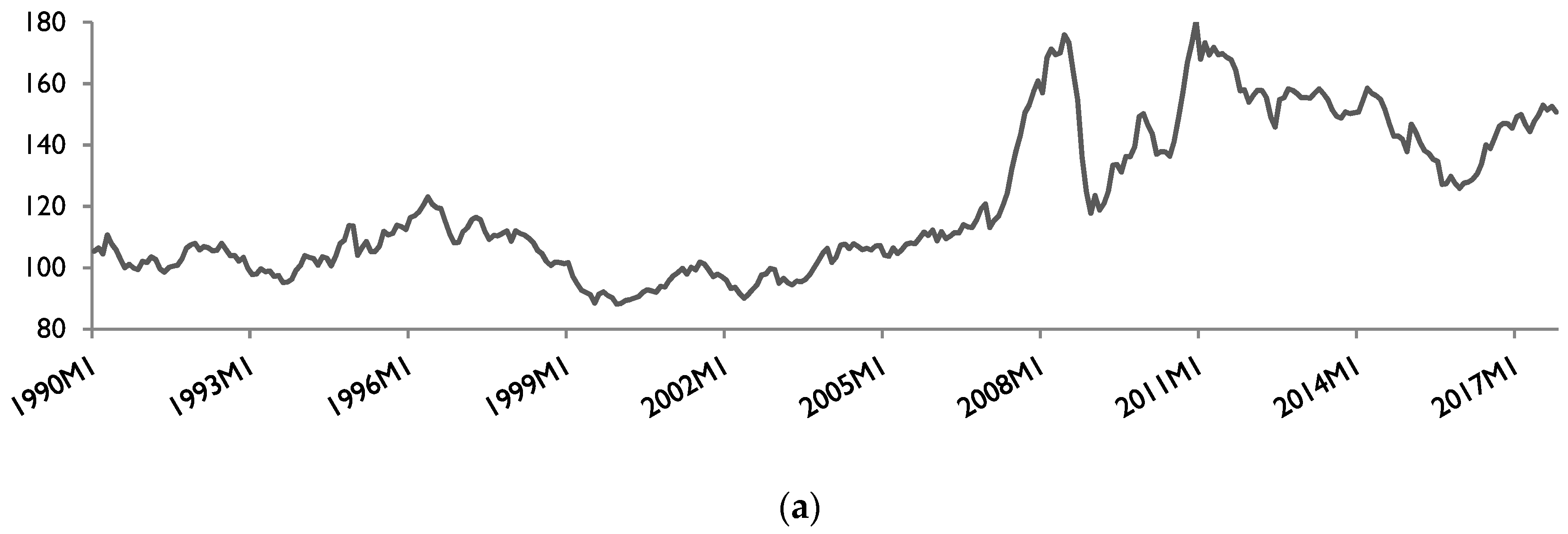
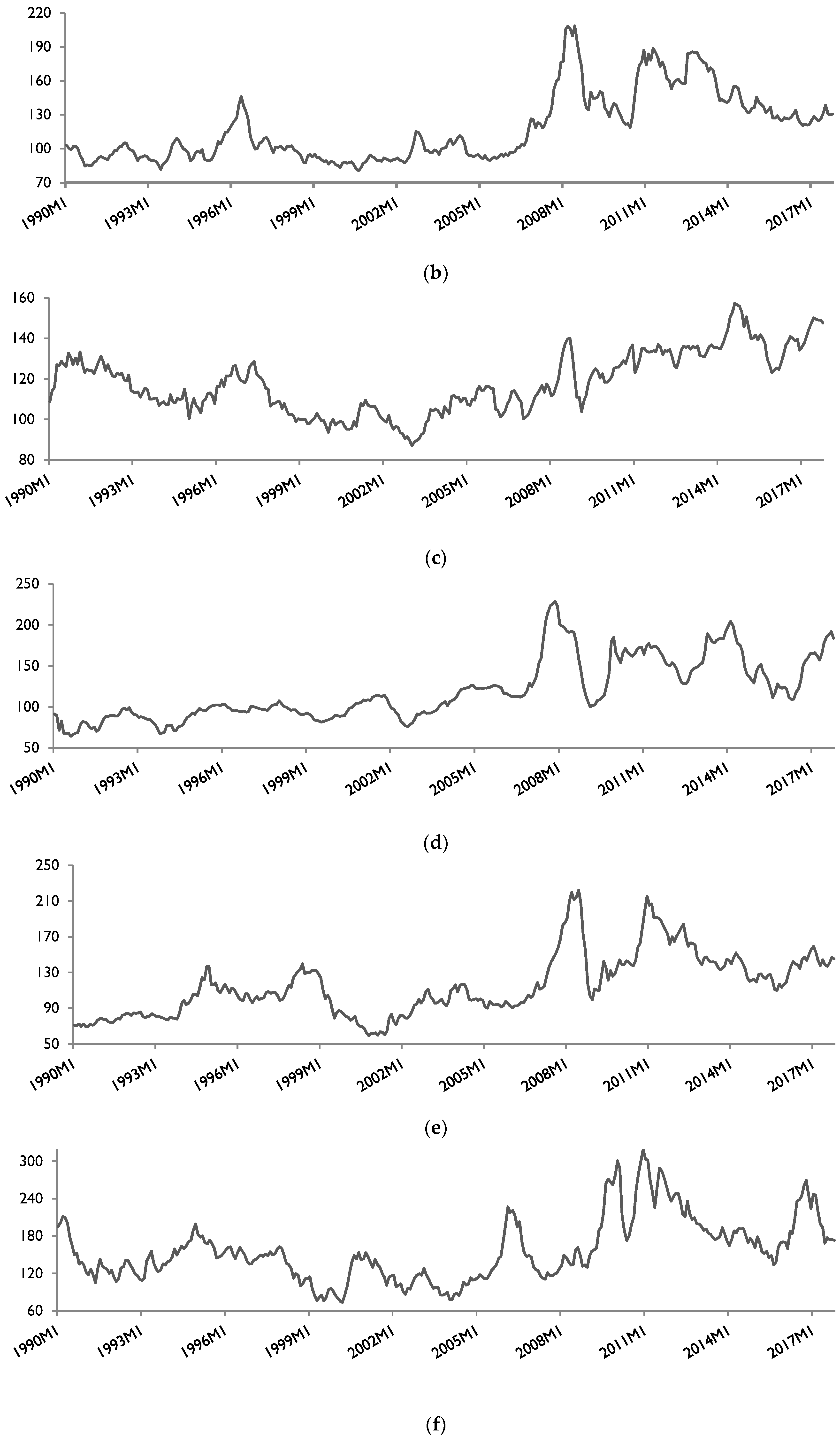
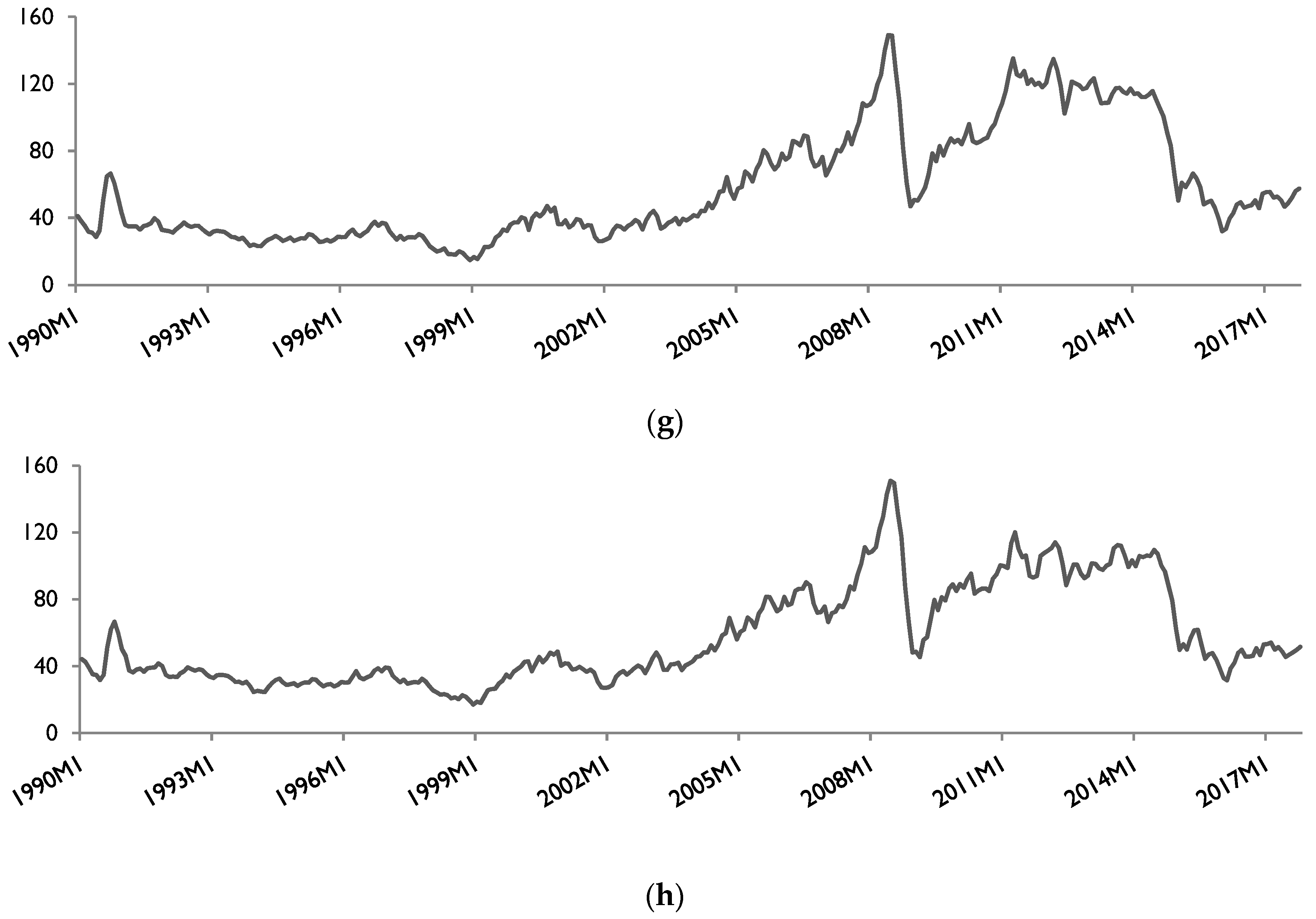
The empirical investigation aims to identify the response of the world food price to oil price fluctuations. Monthly data on the food price index comes from the Food and Agriculture Organization of the United Nations. The analysis considers the overall food price index (FPI) and the price indices of five groups of commodities, namely the meat price index (MPI), the dairy price index (DPI), the cereals price index (CPI), the vegetable oils price index (VOPI) and the sugar price index (SPI). The overall food price index is defined as the average of the different commodity price indices mentioned above and is therefore based on 73 food commodity international prices classified in five main groups, namely meat, vegetable oils, sugar, cereals and dairy. As indicated in the original dataset, all aforementioned price indices have been deflated using the World Bank Manufactures Unit Value Index. Regarding the explanatory variable, this study considers the two most important oil price benchmarks (Brent and West Texas Intermediate (WTI)) to examine the oil price–food price relationship. As pointed out by Ajmi et al. (2014), while the Brent and WTI are the global oil benchmarks and the most used in empirical studies, they may exhibit different behaviors and interact differently with economic and financial variables. Data on the Brent and WTI oil prices are obtained from the Energy Information Administration website. To deflate the nominal prices, we use the U.S. consumer price index obtained from the Federal Reserve Bank of St. Louis. The empirical investigation is based on monthly data covering the period January 1990–October 2017. The choice of the period was not accidental. First and most importantly, the period under study was characterized by sharp fluctuations regarding both oil price and agricultural commodity prices. Indeed, the studied period covers the food price spike episodes (2007–2008, 2010–2012) and oil turmoil periods (1990–1991, 2007–2008, 2014, among others). Second, the period selection was dictated by the availability of disaggregated data on agricultural commodity prices. In fact, the FAO monthly dataset starts from January 1990 (the earliest available for disaggregated agricultural commodity prices). Figure 1 below describes the evolution of the deflated food price indices and oil prices during the studied period.
As shown, the food price index was characterized by an important increasing trend, particularly starting from 2007. The price index increased by about 45% from 113% in 2007M01 to reach 164% in 2008M08, which coincides in time with the world food crisis. There was another rise in the price index in 2010–2011 (more than 180% in December 2010). Regarding the evolution of the various food commodities, it is useful to note that all price indices have also increased, especially during the food crisis episode. The highest increase is observed for the sugar price index and the dairy price index, which reached 319% in December 2010 and 228% in November 2007, respectively. While the meat price index exhibited an increasing trend between 2003 and 2017, it did not exceed 160%. Overall, a rise of the global and sub-indices has been observed over the full period. With reference to the oil price, the same figure shows that until 2003, the Brent and WTI prices remained stable with a slight fall in 1998. However, prices jumped considerably starting from 2003 and settled at a historical record high above $140. In real terms, prices reached $150 per barrel for the Brent crude oil and $149 per barrel for the WTI crude oil in June 2008. The second rise of oil prices occurred in 2011, when they rebounded above $120 per barrel (April 2011). It is useful to mention that the rise of food prices and oil prices occurred in almost the same period. The fall of oil prices after 2008 has been weakly associated with a decrease of almost all food price indices, which gives a preliminary intuition of the presence of asymmetry in the relationship between them.
4. The Empirical Methodology
Most of the previous empirical studies have implicitly presumed the presence of a symmetric impact of oil price on food price. This means that the response of the food price to oil price fluctuations is assumed to be the same whether there is an increase or a decrease of the oil price. The current paper avoids such an assumption by investigating the potential asymmetric impact. The recent developments of the econometric theory allow the estimation of asymmetric relationships between financial and economic variables. More specifically, Shin et al. (2014) developed the nonlinear ARDL approach to study the potential asymmetric effects in both the long and short-run. In fact, the nonlinear ARDL approach is essentially based on the linear ARDL approach developed by Pesaran et al. (2001). The general form of the ARDL (n,m) representation is expressed as
where Δ is the first difference operator, are parameters to be estimated, n and m are the optimal lag length to be used. Theoretically, the absence of cointegrating relationships between and x is confirmed if . To decide whether there is a long-run relationship between the two variables or not, the computed FPSS statistic obtained from the Equation (1) should be compared to the asymptotic critical value bounds of Pesaran et al. (2001). In fact, the authors provide two different sets of asymptotic critical values: a lower bound critical value and an upper bound critical value. If the F-statistic is higher than the upper bound, the null hypothesis of no cointegration is rejected. To check the robustness of results, we also compute the tBDM statistic proposed by Banerjee et al. (1998) to test the presence of a long-run relationship between variables. The corresponding null hypothesis is that against the alternative that .
Compared to traditional cointegration approaches, the linear ARDL modeling has many advantages. The most important is that it is possible to test the presence of cointegration even if variables have different orders of integration (integrated of order zero, one or fractionally integrated). Nevertheless, the ARDL modeling supposes that the impact of on is symmetric and is not able to capture the potential asymmetric effects. Shin et al. (2014) developed the nonlinear ARDL approach which is considered to be an extension of linear ARDL modeling. The authors propose to decompose the explanatory variable as follows:
where and are partial sum processes of positive and negative changes in , obtained as follows:
Therefore, the nonlinear asymmetric long-run equilibrium relationship can be expressed as
where and are the asymmetric long-run parameters associated with positive and negative changes in , respectively. The last step consists of combining Equations (1) and (5) to obtain the following nonlinear ARDL (n, m):
where and are the asymmetric distributed-lag parameters, and are the associated asymmetric long-run parameters.2
The empirical methodology involved four major stages. We start by investigating the stationarity of the time series. Second, we implement the linear ARDL model presented in Equation (1), which allows us to conclude if there is a linear long-run relationship between oil prices and food prices and to estimate short and long-run coefficients. Then, we implement the nonlinear ARDL approach by estimating Equation (6) in order to check if the two variables are nonlinearly cointegrated. Finally, if cointegration exists, we estimate the asymmetric responses of food prices to oil price fluctuations and test the presence of short and long-run asymmetries based on the Wald test.
5. Empirical Results
5.1. Results of Unit Root Tests
Despite the ARDL bounds approach not requiring the pretesting of the integration properties of variables, one should ensure that no variable is integrated at second difference or more. The presence of variables integrated of an order higher than one means that the computed F-statistics are invalid. We perform two kinds of unit root tests, namely unit root tests without structural breaks (augmented Dickey–Fuller (ADF) unit root test and the Elliott, Rothenberg and Stock (ERS) point optimal test) and a unit root with structural break (Zivot and Andrews (1992) unit root (ZA)).3 Results are summarized in Table 1.4
The ADF and ERS unit root tests suggest that the Brent and WTI oil prices, and the food and meat price indices are non-stationary in levels and stationary in first differences. Regarding the other price indices (dairy, cereals, vegetable oils and sugar), the same tests reveal that they are integrated of orders zero or one. Accordingly, Table 1 shows that that none of variables is integrated of order 2 or above. In the same table, we report results of the Zivot and Andrews (1992) structural break unit root. The findings are in line with those of the ADF and ERS unit root tests since variables are found to be integrated of order zero (food, meat and cereals) or one (Brent, WTI, dairy, vegetable oils and sugar). Moreover, it is shown that breaks in data occurred in 2007 for the food, dairy, cereals and vegetable oils price indices; i.e., during the food crisis episode. The oil price variables exhibited a structural break in 2003–2004 and are stationary in first differences. All in all, the different unit root tests reveal that none of the variables are integrated of order 2 or more.
5.2. Linear ARDL Estimates
The next step consists of estimating the following linear ARDL (n,m) model:
where stands for oil prices (Brent or WTI) and stands for food prices (overall food, meat, dairy, cereals, vegetable oils or sugar). Estimation results are presented in Table 2.5
The FPSS and tBDM statistics are found to range between the 10% lower and upper bounds, which means that no conclusion may be drawn on the presence of cointegration between the overall food price index and the Brent and WTI oil prices. This may be explained by the fact that the overall food price index is the combination of an important number of agricultural commodities price indices, and may not capture the real evolution of any of them. The problem of aggregation may be resolved by considering a disaggregated analysis of the main components of the overall food price index. The table also reveals that the evolution of the Brent and WTI oil prices exerts a significant impact on the overall food price index in both the short and long-run. Moreover, two statements should be mentioned. First, the impact of the WTI oil price is higher than that associated with the Brent oil price. In the long-run, a 1% increase (decrease) of the WTI oil price is associated with an increase (decrease) of the overall food price by 0.347% while a 1% increase of the Brent oil price results in an increase of the overall food price by only 0.310%. Second, it is observed that the response of the overall food price index is smaller in the short than in the long-run. The associated coefficients are 0.009 for the Brent oil price and 0.010 for the WTI oil price.
Despite the previous aggregate analysis provides an insight into the reaction of the overall food price index to oil price fluctuations, it seems to be imperative to check the impact of oil price at the disaggregate level. In fact, the different food price indices may react differently to oil prices due to the degree of importance of crude oil as an input for the production process. While oil prices and the different food prices are cointegrated, the magnitude and significance of long-run coefficients vary across the considered commodity. The long-run impacts of oil prices on the dairy price index, the sugar price index and the cereals price index are found to be higher than the average long-run impact of oil prices. The highest impacts of the Brent and WTI oil prices are observed for the dairy commodity price (0.414 for the Brent and 0.455 for the WTI). On the other hand, the lowest impact is associated with the vegetable oil price index (0.234 for the Brent and no significant impact for the WTI). In the short-run, the impact of oil prices on the different food price indices is positive and statistically significant, except for the vegetable oils price index. In addition, the short-run impact of oil prices is smaller than that observed in the long-run. Consequently, the reaction of the food price indices to oil price fluctuations takes place quickly (one to two months after a shock on oil price occurs) but is weak and increases with time to become higher in the long-run. Finally, as in the long-run, the short-run impact of the WTI price index is higher than the Brent oil price. Overall, the linear ARDL bounds testing approach shows that the rise (fall) of oil prices induces a rise (fall) of the global and different food price indices (except vegetable oils) in both the short and long-run. However, the highest impact is observed in the long-run and is associated with the WTI crude oil price.
5.3. Nonlinear ARDL Estimates
While the previous analysis allows the investigation of the effect of oil prices on food prices, it implicitly assumes that the aforementioned impact is symmetric. We avoid such an assumption by decomposing the change in oil price into their partial sum of positive and negative changes and estimating the nonlinear version of the ARDL model. Thus, the following nonlinear ARDL (n,m) is estimated:
The optimal lag length of the nonlinear ARDL (n,m) is chosen based on the Schwarz (1978) information criterion. As in Ibrahim (2015) and Zhang et al. (2017), we then use the general-to-specific approach by dropping all insignificant short-run regressors. Results are presented in Table 3.6
Focusing on the impact of the Brent and WTI oil prices on the overall food price index, the table shows that the FPSS test and tBDM test suggest different results. The FPSS statistic (4.408 for the Brent and 4.152 for the WTI) lies between the lower and upper bounds, suggesting that result is inconclusive for the presence of cointegration. On the contrary, the tBDM test reveals the presence of a long-run nonlinear relationship between the overall food price index on the one hand and the Brent oil price (at the 5% significance level) and the WTI oil price (at the 10% significance level) on the other hand. Consequently, one can admit that the two variables exhibit an asymmetric long-run relationship. The Wald test is then implemented to test the presence of long and short-run asymmetries in the impact of oil prices on the overall food price index. The null hypothesis of this test is the presence of a symmetric impact. According to Table 3, the Wald test rejects the null hypothesis in the long-run for the Brent oil price (at the 5% significance level) and the WTI oil price (at the 1% significance level), which supports the presence of an asymmetric impact of oil prices on the overall food price index in the long-run. In fact, the overall food price reacts differently to positive changes and negative changes of the oil price. In the long-run, it is found that oil price affects the food price index only when it records an increase. The estimated long-run impacts associated with a positive shock on the Brent and WTI oil prices are 0.158 and 0.172, respectively, and are statistically significant at the 5% level. On the other hand, while the impact of negative shocks of oil price is negative, it is not statistically significant. Such findings are of great importance since they reveal that the food price index increases when oil prices jump, but does not follow the oil price when it falls. This point may be confirmed by the inspection of Figure 1, which shows, for instance, that oil prices decreased in early 2013, but the food price index did not. Moreover, these results also provide an argument for the use of the nonlinear ARDL modeling when investigating the impact of oil price on food price. Finally, the Wald test suggests a certain amount of evidence regarding the presence of asymmetry in the impact of oil prices on food price in the short-run. In fact, the null hypothesis cannot be rejected for the WTI oil price, i.e., the short-run impact is symmetric, while for the Brent oil price, the null hypothesis is rejected at the 10% level.
As mentioned earlier, the overall food price index is the average of 73 international food commodity prices included in five categories of commodities, namely meat, dairy, cereals, vegetable oils and sugar. The prices of these commodities may react differently to oil price. It seems then to be useful to investigate the asymmetric response of the different commodity prices to oil prices. The results presented in Table 3 suggest that the null hypothesis of no cointegration cannot be accepted for four food price commodities, namely dairy, cereals, vegetable oils and sugar. On the contrary, the FPSS and tBDM tests reveal that the meat price index and oil prices (Brent and WTI) are not cointegrated, i.e., no long-run asymmetric relationship between them exists. This is also confirmed by the insignificance of long-run coefficients on positive and negative changes of oil prices. Moreover, the Wald test confirms the presence of an asymmetric impact of the Brent and WTI oil prices on the meat price index only in the short-run. This means that the meat price index reacts differently to positive and negative changes of oil price only in the short-run. The table also shows that coefficients of negative shocks on oil price (Brent and WTI) are statistically significant, while those of positive shocks are not. Finally, it is worth noting that the impacts of the Brent and WTI oil prices are closer in the short-run. To summarize, our findings reveal that the meat price index and oil prices do not exhibit a long-run asymmetric relationship and that the asymmetry is present in the short-run since the meat price index responds only to negative changes of the oil price.
Table 3 shows that for the four other food commodities, the FPSS and tBDM tests confirm the presence of a long-run asymmetric relationship with the Brent and WTI oil prices. Nevertheless, some differences between them exist. For the cereals and sugar price indices, while the null hypothesis of no cointegration is rejected, the Wald test confirms the rejection of asymmetries in the relationship between them and the Brent and WTI oil prices in both the short and long-run. Consequently, one may conclude that the response of the cereals price index and sugar price index to oil price fluctuations is symmetric and is identical whether there is an increase or a decrease of oil prices. Regarding the vegetable oils price index, the FPSS and tBDM tests suggest the presence of a long-run asymmetric relationship. However, long-run coefficients associated with the Brent and WTI oil prices are not statistically significant, despite the Wald test indicating the presence of asymmetries in the long-run. The table also confirms the presence of asymmetries in the impact of only the Brent oil price on the vegetable oils price index in the short-run. As in the case of the meat price index, only negative shocks on the oil price are found to affect the vegetable oils price index in the short-run. Finally, we investigate the impact of oil price on the dairy price index. As shown in Table 3, the two cointegration test statistics suggest the rejection of the null hypothesis at the 1% level and confirm the presence of a long-run asymmetric relationship between the two variables. Moreover, the Wald test strongly confirms the asymmetric impact of the Brent and WTI oil prices on the dairy price index. While the dairy price index is affected by both positive and negative changes of the oil price, the impact of positive shocks is higher that associated with negative shocks. This statement remains true whether the WTI or Brent oil price is considered. Moreover, the overall impacts of the WTI oil price are found to be higher than those of the Brent oil price. In the short-run, things seem to be different since the Wald test shows that the asymmetric response of the dairy price index to oil price is observed only for the case of the WTI. Once again, when there are asymmetries in the short-run, the food price index is found to be affected only the negative shocks on oil prices. That is, in the short-run, the dairy price index reacts to the WTI oil price only when it falls.
6. Managerial Implications
From the perspective of international society, our findings underline the need for the implementation of some actions and policies. First, since our findings highlight that the FAO’s overall food price index is only affected by positive shocks on oil price in the long-run, it will be useful to coordinate efforts at the global level to mitigate those effects. For instance, the Organization of the Petroleum Exporting Countries and the Food Agricultural Organization might organize negotiations under the umbrella of the World Trade Organization in order to set a relatively low oil price in favor of the largest producing countries of agricultural commodities. Favorable prices, used only when the spot oil price exceeds a predefined threshold, might alleviate the transmission of oil price increases to agricultural commodities markets. Of course, negotiations should reach a win–win agreement for all parties, since countries that accept to reduce oil prices (particularly OPEC countries) will benefit from reduced agricultural commodity prices in return. The negotiation may be organized by the World Trade Organization to guarantee its application. Second, the main producing countries of basic agricultural commodities, such as cereals and dairy, can partially subsidize agricultural activities in order to control the evolution of agricultural commodity prices during episodes of high oil price volatility.
7. Concluding Remarks
Over the last decades, the world economy has faced sharp fluctuations of agricultural and food commodity prices, which certainly has deteriorated the well-being of people in almost all countries. The occurrence of the food crisis in early 2006 has incited scholars to identify and provide a better understanding of factors responsible for that situation. This paper aims to revisit the aforementioned topic by adopting a relatively recent econometric tool, namely the nonlinear ARDL modeling developed by Shin et al. (2014). By doing so, it relaxes a commonly considered assumption in previous studies, i.e., symmetry, and investigates whether the oil price exerts an asymmetric impact on food prices. Furthermore, the study develops both aggregated and disaggregated analyses by considering the international price of five agricultural commodities during the period ranging from January 1990 to October 2017. For robustness checks, we consider the two most important oil price benchmarks in international markets, namely the Brent and WTI.
Before implementing the nonlinear ARDL, we started by estimating the linear version of the ARDL, which confirmed the presence of a long-run cointegrating relationship between the oil price and the food price indices. However, no conclusions regarding the response of the food price indices to positive and negative changes of the oil price were reached. We then estimated the nonlinear ARDL model for the overall food price index and the price indices of five groups of agricultural commodities, namely meat, dairy, cereals, vegetable oils and sugar. The findings suggested that there is a long-run nonlinear relationship between the overall food price index and the oil prices (Brent and WTI). Moreover, estimates confirmed the presence of an asymmetric impact of oil price on the overall food price index in the long-run, and that this latter is only affected by the rise of oil price. A fall of the WTI and Brent oil prices has no effect the food price. In the short-run, asymmetry is only verified for the Brent oil price, since the overall food price is affected by a fall of the oil price. Regarding the disaggregated analysis, our results show that only the dairy price index, the cereals price index and the vegetable oils have a nonlinear long-run relationship with oil price. From these three agricultural commodities, both the Brent and WTI oil prices are found to exert an asymmetric impact only on the dairy price index in the long-run. While the price index reacts to both positive and negative changes of oil price, the effect of positive shocks is greater than that associated with negative shocks. For the other agricultural commodities, asymmetry is confirmed in some of them, namely meat and vegetable oils. The price of these two commodities reacts only to a fall of oil price in the short-run.
Although the present study offers fresh insights on the impact of oil prices on food prices, it is subject to some limitations related essentially to data and the econometric approach. While monthly data may reflect the evolution of prices, high-frequency data may be more useful. In addition, the nonlinear ARDL is not able to estimate time-varying coefficients. Consequently, evident avenues for future research are to consider daily or weekly datasets when examining the impact of oil price on food prices. Moreover, a more disaggregated dataset on agricultural commodity prices may be of great interest. Finally, combining the nonlinear ARDL approach with time-varying modeling may offer interesting findings on the subject.
Author Contributions
Both authors contributed equally to this research.
Funding
The authors gratefully acknowledge the approval and the support of this research study by the grant no. BA-2017-1-8-F-7215 from the Deanship of Scientific Research at Northern Border University, Arar, K.S.A.
Conflicts of Interest
The authors declare no conflict of interest.
References
- Abbott, Philip C., Christopher Hurt, and Wallace E. Tyner. 2008. What’s Driving Food Prices? Issue Reports 37951. Oak Brook: Farm Foundation. [Google Scholar]
- Abbott, Philip C., Christopher Hurt, and Wallace E. Tyner. 2009. What’s Driving Food Prices? March 2009 Update. Issue Reports 48495. Oak Brook: Farm Foundation. [Google Scholar]
- Abdulai, Awudu. 2000. Spatial price transmission and asymmetry in the Ghanaian maize market. Journal of Development Economics 63: 327–49. [Google Scholar] [CrossRef]
- Ajmi, Ahdi Noomen, Ghassen El-montasser, Shawkat Hammoudeh, and Duc Khuong Nguyen. 2014. Oil prices and MENA stock markets: New evidence from nonlinear and asymmetric causalities during and after the crisis period. Applied Economics 46: 2167–77. [Google Scholar] [CrossRef]
- Apergis, Nicholas, and Anthony Rezitis. 2011. Food price volatility and macroeconomic factors: Evidence from GARCH and GARCH-X estimates. Journal of Agricultural and Applied Economics 43: 95–110. [Google Scholar] [CrossRef]
- Asfaha, T. A., and Andre Jooste. 2007. The effect of monetary changes on relative agricultural prices. Agrekon 46: 460–74. [Google Scholar] [CrossRef]
- Balcombe, Kelvin, and George Rapsomanikis. 2008. Bayesian estimation and selection of nonlinear vector error correction models: The case of sugar–ethanol oil nexus in Brazil. American Journal of Agricultural Economics 90: 658–68. [Google Scholar] [CrossRef]
- Banerjee, Anindya, Juan Dolado, and Ricardo Mestre. 1998. Error-correction mechanism tests for cointegration in a single-equation framework. Journal of Time Series Analysis 19: 267–83. [Google Scholar] [CrossRef]
- Barnett, Richard C., David A. Bessler, and Robert L. Thompson. 1983. The money supply and nominal agricultural prices. American Journal of Agricultural Economics 65: 303–7. [Google Scholar] [CrossRef]
- Baumeister, Christiane, and Lutz Kilian. 2014. Do oil price increases cause higher food prices? Economic Policy 29: 691–747. [Google Scholar] [CrossRef] [Green Version]
- Büyükşahin, Bahattin, and Jeffrey H. Harris. 2011. Do speculators drive crude oil futures prices? Energy Journal 32: 167–202. [Google Scholar] [CrossRef]
- Campiche, Jody L., Henry L. Bryant, James W. Richardson, and Joe L. Outlaw. 2007. Examining the evolving correspondence between petroleum prices and agricultural commodity prices. Paper presented at American Agricultural Economics Association Annual Meeting, Portland, OR, USA, July 29–August 1. [Google Scholar]
- Chen, Sheng-Tung, Hsiao-I Kuo, and Chi-Chung Chen. 2010. Modeling the relationship between the oil price and global food prices. Applied Energy 87: 2517–25. [Google Scholar] [CrossRef]
- Claudio, Araujo, Catherine Araujo-Bonjean, and Johny Egg. 2010. Choc pétrolier externe et performance des marchés des céréales: le marché du mil au Niger. Revue d’économie du développement 18: 47–70. [Google Scholar]
- Coronado, Semei, Omar Rojas, Rafael Romero-Meza, Apostolos Serletis, and Leslie Verteramo Chiu. 2018. Crude oil and biofuel agricultural commodity prices. In Uncertainty, Expectations and Asset Price Dynamics. Edited by Fredj Jawadi. Basel: Springer International Publishing, pp. 107–23. [Google Scholar]
- Deaton, Angus, and Guy Laroque. 1992. On the behaviour of commodity prices. The Review of Economic Studies 59: 1–23. [Google Scholar] [CrossRef]
- Dickey, David A., and Wayne A. Fuller. 1981. Likelihood ratio statistics for autoregressive time series with a unit root. Econometrica 49: 1057–72. [Google Scholar] [CrossRef]
- Diks, Cees, and Valentyn Panchenko. 2006. A new statistic and practical guidelines for nonparametric Granger causality testing. Journal of Economic Dynamics and Control 30: 1647–69. [Google Scholar] [CrossRef]
- Elliott, Graham, Thomas J. Rothenberg, and James H. Stock. 1996. Efficient Tests for an Autoregressive Unit Root. Econometrica 64: 813–36. [Google Scholar] [CrossRef]
- Food and Agriculture Organization of the United Nations (FAO). 2009. The State of Agricultural Commodity Markets, High Food Prices and Food Crisis—Experiences and Lessons Learned. Rome: FAO. [Google Scholar]
- Food Security Information Network. 2018. Global Report on Food Crises 2018. Rome: World Food Programme. [Google Scholar]
- Fowowe, Babajide. 2016. Do oil prices drive agricultural commodity prices? Evidence from South Africa. Energy 104: 149–57. [Google Scholar] [CrossRef]
- Gregory, Allan W., and Bruce E. Hansen. 1996. Residual-based tests for cointegration models with regime shifts. Journal of Econometrics 70: 99–126. [Google Scholar] [CrossRef]
- Hamilton, James D. 1988. Are the macroeconomic effects of oil-price change symmetric? A Comment. Carnegie Rochester Conference Series on Public Policy 28: 369–78. [Google Scholar] [CrossRef]
- Hamilton, James D. 1996. This is what happened to the oil price-macroeconomy relationship. Journal of Monetary Economics 38: 215–20. [Google Scholar] [CrossRef]
- Harri, Ardian, Lanier Nalley, and Darren Hudson. 2009. The relationship between oil, exchange rates, and commodity prices. Journal of Agricultural and Applied Economics 41: 501–10. [Google Scholar] [CrossRef]
- Hoover, Kevin D. 2001. Causality in Macroconomics. Cambridge: Cambridge University Press. [Google Scholar]
- Ibrahim, Mansor H. 2015. Oil and food prices in Malaysia: A nonlinear ARDL analysis. Agricultural and Food Economics 3: 1–14. [Google Scholar] [CrossRef]
- Johansen, Soren. 1988. Statistical analysis of cointegration vectors. Journal of Economic Dynamics and Control 12: 231–54. [Google Scholar] [CrossRef]
- Johansen, Soren. 1991. Estimation and hypothesis testing of cointegration vectors in Gaussian vector autoregressive models. Econometrica 59: 1551–80. [Google Scholar] [CrossRef]
- Koirala, Krishna H., Ashok K. Mishra, Jeremy M. D’Antoni, and Joey E. Mehlhorn. 2015. Energy prices and agricultural commodity prices: Testing correlation using copulas method. Energy 81: 430–36. [Google Scholar] [CrossRef]
- Kripfganz, Sebastian, and Daniel C. Schneider. 2016. ardl: Stata module to estimate autoregressive distributed lag models. Paper presented at Stata Conference, Chicago, IL, USA, July 29. [Google Scholar]
- Lagi, Marco, Yavni Bar-Yam, Karla Z. Bertrand, and Yaneer Bar-Yam. 2015. Accurate market price formation model with both supply-demand and trend-following for global food prices providing policy recommendations. Proceedings of the National Academy of Sciences 112: E6119–28. [Google Scholar] [CrossRef]
- Mills, Terence C. 1991. Nonlinear time series models in economics. Journal of Economic Surveys 5: 215–42. [Google Scholar] [CrossRef]
- Narayan, Seema, and Paresh Kumar Narayan. 2007. Understanding asymmetries in macroeconomic aggregates: The case of Singapore. Applied Economics Letters 14: 905–8. [Google Scholar] [CrossRef]
- Nazlioglu, Saban. 2011. World oil and agricultural commodity prices: Evidence from nonlinear causality. Energy Policy 39: 2935–43. [Google Scholar] [CrossRef]
- Nazlioglu, Saban, and Ugur Soytas. 2011. World oil prices and agricultural commodity prices: Evidence from an emerging market. Energy Economics 33: 488–96. [Google Scholar] [CrossRef]
- Pal, Debdatta, and Subrata K. Mitra. 2017. Time-frequency contained co-movement of crude oil and world food prices: A wavelet-based analysis. Energy Economics 62: 230–39. [Google Scholar] [CrossRef]
- Pal, Debdatta, and Subrata K. Mitra. 2018. Interdependence between crude oil and world food prices: A detrended cross correlation analysis. Physica A: Statistical Mechanics and its Applications 492: 1032–44. [Google Scholar] [CrossRef]
- Pala, Aynur. 2013. Structural Breaks, Cointegration, and Causality by VECM Analysis of Crude Oil and Food Price. International Journal of Energy Economics and Policy 3: 238–46. [Google Scholar]
- Paris, Anthony. 2018. On the link between oil and agricultural commodity prices: Do biofuels matter? International Economics 155: 48–60. [Google Scholar] [CrossRef]
- Pesaran, M. Hashem, Yongcheol Shin, and Richard J. Smith. 2001. Bounds testing approaches to the analysis of level relationships. Journal of Applied Econometrics 16: 289–326. [Google Scholar] [CrossRef] [Green Version]
- Rapsomanikis, George, David Hallam, and Piero Conforti. 2003. Market integration and price transmission in selected food and cash crop markets of developing countries: Review and applications. In Commodity Market Review 2003–2004. Rome: FAO. [Google Scholar]
- Reboredo, Juan C. 2012. Do food and oil prices co-move? Energy Policy 49: 456–67. [Google Scholar] [CrossRef]
- Saghaian, Sayed H. 2010. The impact of the oil sector on commodity prices: Correlation or causation? Journal of Agricultural and Applied Economics 42: 477–85. [Google Scholar] [CrossRef]
- Salisu, Afees A., Kazeem O. Isah, Oluwatomisin J. Oyewole, and Lateef O. Akanni. 2017. Modelling oil price-inflation nexus: The role of asymmetries. Energy 125: 97–106. [Google Scholar] [CrossRef]
- Scherer, Frederic M., and David Ross. 1990. Industrial Market Structure and Economic Performance, 3rd ed. Boston: Houghton Mifflin. [Google Scholar]
- Schmidhuber, Josef, and Francesco N. Tubiello. 2007. Global food security under climate change. Proceedings of the National Academy of Sciences 104: 19703–8. [Google Scholar] [CrossRef]
- Schwarz, Gideon. 1978. Estimating the dimension of a model. The Annals of Statistics 6: 461–64. [Google Scholar] [CrossRef]
- Sek, Siok Kun. 2017. Impact of oil price changes on domestic price inflation at disaggregated levels: Evidence from linear and nonlinear ARDL modeling. Energy 130: 204–17. [Google Scholar] [CrossRef]
- Shin, Yongcheol, Byungchul Yu, and Matthew Greenwood-Nimmo. 2014. Modelling asymmetric cointegration and dynamic multipliers in an ARDL framework. In Festschrift in Honor of Peter Schmidt. Edited by Robin C. Sickles and William C. Horrace. New York: Springer Science and Business Media. [Google Scholar]
- Tatom, John A. 1988. Are the macroeconomic effects of oil price changes symmetric? Carnegie-Rochester Conference Series on Public Policy 28: 325–68. [Google Scholar] [CrossRef]
- Tiwari, Aviral Kumar, Rabeh Khalfaoui, Sakiru Adebola Solarin, and Muhammad Shahbaz. 2018. Analyzing the time-frequency lead–lag relationship between oil and agricultural commodities. Energy Economics 76: 470–94. [Google Scholar] [CrossRef]
- Toda, Hiro Y., and Taku Yamamoto. 1995. Statistical inference in vector autoregressive with possibly integrated processes. Journal of Econometrics 66: 225–50. [Google Scholar] [CrossRef]
- Wheeler, Tim, and Joachim von Braun. 2013. Climate change impacts on global food security. Science 341: 508–13. [Google Scholar] [CrossRef]
- Wong, K. Kai Seng, and Mad Nasir Shamsudin. 2017. Impact of crude oil price, exchange rates and real GDP on Malaysia’s food price fluctuations: Symmetric or Asymmetric? International Journal of Economics and Management 11: 259–75. [Google Scholar]
- Zhang, Zan, Su-Ling Tsai, and Tsangyao Chang. 2017. New evidence of interest rate pass-through in Taiwan: A Nonlinear Autoregressive Distributed Lag Model. Global Economic Review 46: 129–42. [Google Scholar] [CrossRef]
- Zivot, Eric, and Donald W. K. Andrews. 1992. Further evidence of great crash, the oil price shock and unit root hypothesis. Journal of Business and Economic Statistics 10: 251–70. [Google Scholar]
| 1 | According to Hoover (2001), the Simpson Paradox refers to “a number of situations in which statistical dependencies that are consistent in subpopulations disappear or are reversed in whole populations” (Hoover 2001, p. 19). |
| 2 | See Shin et al. (2014) for more details. |
| 3 | See Dickey and Fuller (1981), Elliott et al. (1996) and Zivot and Andrews (1992) for details on the construction of unit root tests. |
| 4 | The statistical software Eviews 10 was used to perform unit root tests. |
| 5 | The computations were done in Stata 14 using the ARDL command for Stata (ardl) written by Kripfganz and Schneider (2016). |
| 6 | The computations were done in Stata 14 using the nonlinear ARDL command for Stata (nardl) written by Marco Sunder and retrieved from Matthew Greenwood-Nimmo’s webpage. |
Figure 1.
Plots of variables. (a) Food price index; (b) cereals price index; (c) meat price index; (d) dairy price index; (e) vegetable oils price index; (f) sugar price index; (g) Brent crude oil price (US$ per barrel); (h) West Texas Intermediate (WTI) crude oil price (US$ per barrel).
Figure 1.
Plots of variables. (a) Food price index; (b) cereals price index; (c) meat price index; (d) dairy price index; (e) vegetable oils price index; (f) sugar price index; (g) Brent crude oil price (US$ per barrel); (h) West Texas Intermediate (WTI) crude oil price (US$ per barrel).


Table 1.
Results of unit root tests.
| ADF | ERS | ZA | ||||||
|---|---|---|---|---|---|---|---|---|
| Level | 1st Diff. | Level | 1st Diff. | Level | Break Date | 1st Diff. | Break Date | |
| lnBrent | −2.641 | −14.000 *** | 8.464 | 0.277 *** | −3.831 | 2004M07 | −14.197 *** | 1999M01 |
| lnWTI | −2.732 | −13.506 *** | 7.816 | 0.204 *** | −4.093 | 2003M10 | −8.364 *** | 1999M01 |
| lnFPI | −2.453 | −14.476 *** | 10.513 | 0.190 *** | −5.084 ** | 2007M02 | −8.362 *** | 2008M07 |
| lnMPI | −2.162 | −16.695 *** | 9.839 | 0.561 *** | −5.398 ** | 2001M10 | −5.346 *** | 2003M04 |
| lnDPI | −3.716 ** | −12.777 *** | 4.491 ** | 0.217 *** | −4.503 | 2007M02 | −12.960 *** | 2007M12 |
| lnCPI | −2.965 | −13.253 *** | 6.481 * | 0.223 *** | −5.334 ** | 2007M05 | −13.487 *** | 2008M03 |
| lnVOPI | −3.565 ** | −7.008 *** | 3.129 *** | 0.348 *** | −4.259 | 2007M04 | −7.616 *** | 2001M06 |
| lnSPI | −3.521 ** | −14.145 *** | 7.922 | 0.184 *** | −4.714 | 2009M01 | −14.277 *** | 2011M01 |
Notes: ADF, ERS and ZA are the augmented Dickey–Fuller test, the Elliott et al. (1996) point optimal unit root test and the Zivot and Andrews (1992) structural breaks test. Break denotes the date of the break for the ZA unit root test. The optimal lag length is determined using the Akaike lag length selection criteria. *, ** and *** denote the rejection of the null hypothesis at 10%, 5% and 1% significance levels, respectively.
Table 2.
The linear autoregressive distributed lag (ARDL) estimation results.
| Variable | Brent Crude Oil | WTI Crude Oil | ||||
|---|---|---|---|---|---|---|
| Coefficient | t-Statistic | p-Value | Coefficient | t-Statistic | p-Value | |
| Dependent variable: ΔFPI | ||||||
| Constant | 0.115 *** | 2.68 | 0.008 | 0.102** | 2.53 | 0.012 |
| lnFPIt−1 | −0.032 *** | −2.86 | 0.005 | −0.029 *** | −2.78 | 0.006 |
| lnOPt−1 | 0.310 *** | 4.03 | 0.000 | 0.347 *** | 3.71 | 0.000 |
| ΔlnFPIt−1 | 0.243 *** | 4.56 | 0.000 | 0.242 *** | 4.53 | 0.000 |
| ΔlnOPt−1 | 0.009 ** | 2.58 | 0.010 | 0.010 ** | 2.51 | 0.012 |
| Cointegration test statistics | FPSS = 4.240 tBDM = −2.857 | FPSS = 4.076 tBDM = −2.781 | ||||
| Dependent variable: ΔMPI | ||||||
| Constant | 0.163 *** | 2.75 | 0.006 | 0.101 * | 1.73 | 0.085 |
| lnMPIt−1 | −0.043 *** | −3.18 | 0.002 | −0.028 ** | −2.13 | 0.034 |
| lnOPt−1 | 0.252 *** | 3.53 | 0.001 | 0.314 ** | 2.31 | 0.021 |
| ΔlnOPt−1 | 0.010 *** | 3.49 | 0.001 | 0.034 * | 1.85 | 0.065 |
| ΔlnOPt−1 | − | − | - | 0.056 *** | 3.01 | 0.003 |
| Cointegration test statistics | FPSS = 7.416 ** tBDM = −3.180 * | FPSS = 3.878 tBDM = −2.127 | ||||
| Dependent variable: ΔDPI | ||||||
| constant | 0.147 *** | 3.76 | 0.000 | 0.133 *** | 3.55 | 0.000 |
| lnDPIt−1 | −0.046 *** | −4.01 | 0.000 | −0.044 *** | −3.89 | 0.000 |
| lnOPt−1 | 0.414 *** | 5.14 | 0.000 | 0.455 *** | 4.83 | 0.000 |
| ΔlnDPIt−1 | 0.496 *** | 10.40 | 0.000 | 0.497 *** | 10.39 | 0.000 |
| ΔlnOPt−1 | 0.019 *** | 3.16 | 0.002 | 0.020 *** | 3.01 | 0.003 |
| Cointegration test statistics | FPSS = 8.040 *** tBDM = −4.010 *** | FPSS = 7.570 ** tBDM = −3.890 *** | ||||
| Dependent variable: ΔCPI | ||||||
| Constant | 0.152 *** | 3.13 | 0.002 | 0.137 *** | 2.98 | 0.003 |
| lnCPIt−1 | −0.043 *** | −3.29 | 0.001 | −0.041 *** | −3.23 | 0.001 |
| lnOPt−1 | 0.326 *** | 3.80 | 0.000 | 0.360 *** | 3.53 | 0.000 |
| ΔlnCPIt−1 | 0.326 *** | 6.25 | 0.000 | 0.325 *** | 6.22 | 0.000 |
| ΔlnOPt−1 | 0.014** | 2.50 | 0.013 | 0.014** | 2.43 | 0.016 |
| Cointegration test statistics | FPSS = 5.405 * tBDM = −3.287 ** | FPSS = 5.226 * tBDM = −3.231 ** | ||||
| Dependent variable: ΔVOPI | ||||||
| Constant | 0.143 *** | 3.08 | 0.002 | 0.136 *** | 2.97 | 0.003 |
| lnVOPIt−1 | −0.037 *** | −3.10 | 0.002 | −0.035 *** | −3.01 | 0.003 |
| lnOPt−1 | 0.234 * | 1.78 | 0.076 | 0.238 | 1.53 | 0.126 |
| ΔlnVOPIt−1 | 0.343 *** | 6.33 | 0.000 | 0.343 *** | 6.32 | 0.000 |
| ΔlnVOPIt−2 | −0.140 ** | −2.45 | 0.015 | −0.141 ** | −2.47 | 0.014 |
| ΔlnVOPIt−4 | 0.173 *** | 3.19 | 0.002 | 0.172 *** | 3.16 | 0.002 |
| ΔlnOPt−1 | 0.008 | 1.44 | 0.151 | 0.008 | 1.27 | 0.205 |
| Cointegration test statistics | FPSS = 4.956 * tBDM = −3.099 * | FPSS = 4.721 tBDM = −3.011 * | ||||
| Dependent variable: ΔSPI | ||||||
| Constant | 0.194 *** | 3.03 | 0.003 | 0.180 *** | 2.82 | 0.005 |
| lnSPIt−1 | −0.052 *** | −3.52 | 0.000 | −0.051 *** | −3.50 | 0.001 |
| lnOPt−1 | 0.336 ** | 2.49 | 0.013 | 0.375 ** | 2.40 | 0.017 |
| ΔlnSPIt−1 | 0.262 *** | 4.94 | 0.000 | 0.260 *** | 4.92 | 0.000 |
| ΔlnOPt−1 | 0.017 ** | 2.12 | 0.035 | 0.019 *** | 2.82 | 0.005 |
| Cointegration test statistics | FPSS = 6.253 ** tBDM = −3.522 ** | FPSS = 6.214 ** tBDM = −3.497 ** | ||||
Notes: FPSS and tBDM denote the F-statistic proposed by Pesaran et al. (2001) and the t-statistic proposed by Banerjee et al. (1998). *, ** and *** denote the statistical significance at 10%, 5% and 1% significance levels, respectively.
Table 3.
The nonlinear ARDL estimation results.
| Variable | Brent Crude Oil | WTI Crude Oil | ||||
|---|---|---|---|---|---|---|
| Coefficient | t-Statistic | p-Value | Coefficient | t-Statistic | p-Value | |
| Dependent variable: ΔFPI | ||||||
| Constant | 0.211 *** | 3.58 | 0.000 | 0.201 *** | 3.46 | 0.001 |
| lnFPIt−1 | −0.045 *** | −3.57 | 0.000 | −0.043 *** | −3.45 | 0.001 |
| 0.007 * | 1.78 | 0.077 | 0.007 * | 1.77 | 0.078 | |
| 0.005 | 1.34 | 0.180 | 0.005 | 1.32 | 0.187 | |
| ΔlnFPIt−1 | 0.171 *** | 3.13 | 0.002 | 0.167 *** | 3.03 | 0.003 |
| ΔlnFPIt−2 | 0.106 * | 1.93 | 0.055 | 0.105 * | 1.90 | 0.058 |
| Δ | −0.020 | −0.70 | 0.484 | −0.028 | −0.90 | 0.370 |
| Δ | 0.089 *** | 3.18 | 0.002 | 0.104 *** | 3.50 | 0.001 |
| Cointegration test statistics | FPSS = 4.408 tBDM = −3.565 ** | FPSS = 4.152 tBDM = −3.451 * | ||||
| Long-run asymmetric coefficients | = 0.158 ** = −0.126 | = 0.172 ** = −0.134 | ||||
| Long and short-run asymmetry tests | = 5.705 ** = 2.918 * | = 7.065 *** = 2.256 | ||||
| Dependent variable: ΔMPI | ||||||
| Constant | 0.138 ** | 2.01 | 0.045 | 0.126 * | 1.86 | 0.064 |
| lnMPIt−1 | −0.028 ** | −1.98 | 0.049 | −0.026 * | −1.81 | 0.071 |
| 0.006 | 1.53 | 0.127 | 0.006 | 1.61 | 0.108 | |
| 0.005 | 1.27 | 0.204 | 0.006 | 1.33 | 0.185 | |
| ΔlnMPIt−5 | −0.131 ** | −2.45 | 0.015 | −0.134 ** | −2.52 | 0.012 |
| Δ | 0.040 | 1.23 | 0.219 | 0.040 | 1.23 | 0.219 |
| Δ | 0.060 * | 1.81 | 0.071 | 0.057 * | 1.66 | 0.099 |
| Δ | 0.083 *** | 2.63 | 0.009 | 0.079 ** | 2.37 | 0.018 |
| Cointegration test statistics | FPSS = 2.247 tBDM = −1.976 | FPSS = 2.343 tBDM = −1.808 | ||||
| Long-run asymmetric coefficients | = 0.210 = −0.195 | = 0.253 = −0.231 | ||||
| Long and short-run asymmetry tests | = 0.428 = 3.152 * | = 0.711 = 3.659 * | ||||
| Dependent variable: ΔDPI | ||||||
| Constant | 0.368 *** | 4.99 | 0.000 | 0.395 *** | 5.23 | 0.000 |
| lnDPIt−1 | −0.081 *** | −4.99 | 0.000 | −0.087 *** | −5.22 | 0.000 |
| 0.019 *** | 2.73 | 0.007 | 0.022 *** | 2.97 | 0.003 | |
| 0.015 ** | 2.12 | 0.035 | 0.018 ** | 35 | 0.020 | |
| ΔlnDPIt−1 | 0.289 *** | 5.59 | 0.000 | 0.280 *** | 5.43 | 0.000 |
| ΔlnDPIt−2 | 0.192 *** | 3.66 | 0.000 | 0.194 *** | 3.72 | 0.000 |
| Δ | −0.028 | −0.56 | 0.578 | −0.082 | −51 | 0.131 |
| Δ | 0.067 | 1.40 | 0.163 | 0.121 ** | 36 | 0.019 |
| Cointegration test statistics | FPSS= 8.308 *** tBDM = −4.986 *** | FPSS = 9.113 *** tBDM = −5.216 *** | ||||
| Long-run asymmetric coefficients | = 0.235 ** = −0.189 ** | = 0.262 *** = −0.210 *** | ||||
| Long and short-run asymmetry tests | = 13.21 *** = 0.742 | = 18.63 *** = 2.723 * | ||||
| Dependent variable: ΔCPI | ||||||
| Constant | 0.274 *** | 4.17 | 0.000 | 0.259 *** | 4.02 | 0.000 |
| lnCPIt−1 | −0.058 *** | −4.11 | 0.000 | −0.056 *** | −3.96 | 0.000 |
| 0.015 ** | 2.43 | 0.020 | 0.015 ** | 41 | 0.016 | |
| 0.013 ** | 2.10 | 0.037 | 0.014 ** | 2.08 | 0.039 | |
| ΔlnCPIt−1 | 0.283 *** | 5.22 | 0.000 | 0.289 *** | 5.30 | 0.000 |
| ΔlnCPIt−2 | 0.120 ** | 2.19 | 0.029 | 0.113 ** | 2.05 | 0.041 |
| Δ | −0.068 | −1.48 | 0.140 | −0.049 | −1.01 | 0.315 |
| Δ | 0.095 ** | 2.20 | 0.028 | 0.102 ** | 2.22 | 0.027 |
| Δ | −0.081 * | −1.86 | 0.064 | −0.089 * | −1.95 | 0.052 |
| Cointegration test statistics | FPSS = 5.653 * tBDM =−4.113 *** | FPSS = 5.279 * tBDM = −3.964 *** | ||||
| Long-run asymmetric coefficients | = 0.256 *** = −0.235 ** | = 0.279 *** = −0.254 ** | ||||
| Long and short-run asymmetry tests | = 1.727 = 1.609 | = 2.240 = 0.699 | ||||
| Dependent variable: ΔVOPI | ||||||
| Constant | 0.230 *** | 3.79 | 0.000 | 0.213 *** | 3.53 | 0.000 |
| lnVOPIt−1 | −0.049 *** | −3.72 | 0.000 | −0.046 *** | −3.50 | 0.001 |
| 0.001 | 0.22 | 0.822 | 0.002 | 03 | 0.741 | |
| −0.001 | −0.15 | 0.878 | −0.0003 | .04 | 0.965 | |
| ΔlnVOPIt−1 | 0.339 *** | 6.20 | 0.000 | 0.343 *** | 6.26 | 0.000 |
| ΔlnVOPIt−2 | −0.162 *** | −2.81 | 0.005 | −0.164 *** | −2.81 | 0.005 |
| ΔlnVOPIt−3 | −0.162 *** | −2.81 | 0.005 | 0.098 * | 1.71 | 0.089 |
| ΔlnVOPIt−4 | − | − | 0.161 *** | 2.91 | 0.004 | |
| Δ | −0.041 | −0.69 | 0.494 | −0.041 | −0.65 | 0.514 |
| Δ | 0.173 *** | 3.06 | 0.002 | 0.185 *** | 07 | 0.002 |
| Δ | 0.113 * | 1.86 | 0.064 | 0.094 | 48 | 0.139 |
| Cointegration test statistics | FPSS = 4.794 * tBDM = −3.794 ** | FPSS = 4.215 tBDM = −3.501 ** | ||||
| Long-run asymmetric coefficients | = 0.032 = 0.024 | = 0.053 = 0.008 | ||||
| Long and short-run asymmetry tests | = 5.127 ** = 4.171 ** | = 5.106 ** = 1.462 | ||||
| Dependent variable: ΔSPI | ||||||
| Constant | 0.277 *** | 3.73 | 0.000 | 0.269 *** | 3.64 | 0.000 |
| lnSPIt−1 | −0.056 *** | −3.78 | 0.000 | −0.055*** | −3.72 | 0.000 |
| 0.012 | 1.21 | 0.277 | 0.014 | 31 | 0.192 | |
| 0.010 | 0.94 | 0.347 | 0.012 | 02 | 0.307 | |
| ΔlnSPIt-1 | 0.262 *** | 4.94 | 0.000 | 0.262 *** | 4.92 | 0.000 |
| Δ | −0.099 | −1.13 | 0.258 | −0.041 | .44 | 0.661 |
| Δ | 0.244 *** | 2.97 | 0.003 | 0.189 ** | 18 | 0.030 |
| Cointegration test statistics | FPSS = 4.859 * tBDM = −3.783 ** | FPSS = 4.719 tBDM = −3.718 ** | ||||
| Long-run asymmetric coefficients | = 0.220 = −0.190 | = 0.254 = −0.219 | ||||
| Long and short-run asymmetry tests | = 0.936 = 0.974 | = 1.176 = 0.168 | ||||
Notes: The superscripts “+” and “−” represent the positive and negative partial sums. LR+ and LR− denote the long-run coefficients associated with positive and negative partial sums, while WLR and WSR are the Wald test for long- and short-run symmetry. *, ** and *** denote the statistical significance at 10%, 5% and 1% significance levels, respectively.
© 2019 by the authors. Licensee MDPI, Basel, Switzerland. This article is an open access article distributed under the terms and conditions of the Creative Commons Attribution (CC BY) license (http://creativecommons.org/licenses/by/4.0/).
Share and Cite
MDPI and ACS Style
Zmami, M.; Ben-Salha, O. Does Oil Price Drive World Food Prices? Evidence from Linear and Nonlinear ARDL Modeling. Economies 2019, 7, 12. https://doi.org/10.3390/economies7010012
AMA Style
Zmami M, Ben-Salha O. Does Oil Price Drive World Food Prices? Evidence from Linear and Nonlinear ARDL Modeling. Economies. 2019; 7(1):12. https://doi.org/10.3390/economies7010012
Chicago/Turabian StyleZmami, Mourad, and Ousama Ben-Salha. 2019. "Does Oil Price Drive World Food Prices? Evidence from Linear and Nonlinear ARDL Modeling" Economies 7, no. 1: 12. https://doi.org/10.3390/economies7010012
Note that from the first issue of 2016, this journal uses article numbers instead of page numbers. See further details here.