1. Introduction
Supply networks exist throughout society in manufacturing and knowledge-intensive industries as well as many service industries. Manufacturing and material production supply networks are arguably more straightforward to understand than knowledge- and information-intensive networks as relationships tend to be more clearly defined. Examples of these knowledge- and information-intensive networks include product development, real-estate, healthcare, news/media, and investment services. In these networks, information and knowledge is more difficult to track as it moves through the network. Thoroughly understanding supply network behavior and dependencies are critical to managing such systems effectively. Unfortunately, supply networks often take on the behavior of complex adaptive systems making them more difficult to analyze and assess. Being able to fully understand both the static and dynamic structures of a complex adaptive supply network is critical to being able to make more informed management decisions and prioritize resources and production throughout the network.
1.1. Complex Adaptive Supply Networks
As a starting point, Choi et al. [
1] state that a complex adaptive supply network (CASN) is a collection of firms that seek to maximize their individual profit and livelihood by exchanging information, products, and services with one another. They further elaborate that a larger component of the order in a CASN is the emergent, dynamic, and unpredictable order that arises when the nature of interactions between firms determines the behavior of the network as a whole. In these ways, these interconnected entities exhibit adaptive action in response to changes in both the environment and the system of entities itself.
According to Surana et al. [
2] in a complex adaptive system (CAS), the network elements are dynamic with the states of both the nodes and edges changing with time. They further argue, supply-chain networks form a CAS because they display the following characteristics: structures spanning several scales, strongly coupled degrees of freedom and correlations over long length and timescales, coexistence of competition and cooperation, nonlinear dynamics involving interrelated spatial and temporal effects, quasi-equilibrium and combination of regularity and randomness (i.e., interplay of chaos and non-chaos), emergent behavior and self-organization, and adaption and evolution.
These are similar to the properties noted by Pathak et al. [
3]: a CAS consists of entities that may evolve over time and interact with other entities and the environment by following a set of simple decision rules; a CAS is self-organizing as a consequence of interactions between entities; a CAS coevolves with its environment to the edge of chaos; a CAS is recursive by nature and recombines and evolves over time.
Surana et al. noted several options which exist for modeling CASN: system dynamics, agent-based modeling, deterministic models, and network models. A drawback to system dynamics models is that the structure has to be determined before starting the simulation.
Agent-based models and NK models offer additional approaches to studying supply chains as complex adaptive systems. Mari et al. [
4] used agent-based simulation to test various models of resiliency metrics in complex supply chains. Li et al. [
5] proposed a model for CASN evolution using the principles of CAS and fitness landscape theory. Giannoccaro has used agent-based models to simulate learning in adaptive supply chains [
6] and NK simulation to study supply chain integration and governance [
7]. NK simulation has been also used to study supply chain interdependence/trust [
8,
9].
Hearnshaw et al. [
10] provided a conceptual approach to supply chain network theory drawing on an understanding of complex network theory and adaptive systems. They provide a justification for applying advances in complex network science to supply chain management, but given their conceptual approach, stopped short of empirically validating the many propositions they presented in the research. Providing a quantitative validation of their propositions through modeling or empirical analysis remains an open issue.
However, according to Pathak et al., there are at least three major challenges critical to CASN research. First, the complexity of supply networks pushes the limits of researchers’ ability to understand the internal interactions between constructs and mechanisms or larger-scope phenomena. Second, operations management and supply-chain management lack metrics for evolution and dynamism in supply networks. Third, developing robust theories in the presence of adaptation is a formidable task.
Additionally, Bellamy et al. [
11] identified other research gaps in the area of network science and supply chain management. Overall, they noted that future work should focus on supply chain network structure, supply chain network dynamics, and supply chain network strategy. Since then, recent studies of supply network structures have primarily utilized social network analysis methods. For example, Basole et al. [
12] used a network analysis approach to study the relationships between network structure, risk diffusion, and network health. Bellamy et al. [
13] also used a social network approach to examine how supply chain network structure impacts innovation within the firm.
The obvious drawback of the social network analysis approach is it requires complete knowledge of the network structure in order to be effective. However, in a CASN where both the edges and nodes are dynamic, a complete understanding of the network structure may not be known. To address these difficult issues of complex network structures and dynamics, the authors appeal to the concepts of information dynamics.
1.2. Information Dynamics
Information dynamics arises out of concepts in information theory [
14] such as mutual information,
I(X;Y), (Equation (1)) and conditional mutual information,
I(X;Y|Z), (Equation (2)). In these equations, processes
X,
Y, and
Z have time-series realizations
x,
y, and
z over all possible states α
x, α
y, and α
z. Lizier [
15] describes mutual information as a measure of the information contained in
X about
Y (or vice versa) and the conditional mutual information as the mutual information between
X and
Y when
Z is known.
Additionally, Lizier [
15] describes transfer entropy (Equation (3)) [
16] as the amount of information a source process’ past,
Yn(l), provides about the next state of a destination (or target) process,
X(n+1), in the context of the destination’s past,
Xn(k). In this equation
k and
l are the history lengths of
X and
Y, respectively, while
n is the current time index. Other useful definitions of transfer entropy describe it as a measure of deviation from independence [
17] or as an observed correlation between two processes rather than a direct effect [
18].
Additionally, local transfer entropy (Equation (4)) [
15] defines transfer entropy at each time step
n using the past realizations
xn(k) and the past realizations
yn(k) to quantify the information contained in the source,
Y, about the next state of the destination,
X, at time step
n+1. The local transfer entropy measure gives insight into network structure dynamics and how the correlation and influence or two processes are changing over that time series. This is because local transfer entropy provides a time history of transfer entropy values which quantifies the observed correlation (or influence) between two processes.
Transfer entropy has been implemented with a method to determine the statistical significance of the process relationships being studied. A null hypothesis testing approach has been taken in the Java Information Dynamics Toolkit (JIDT) [
15]. In order to determine if the transfer entropy calculated between two processes is statistically different from
0 (i.e., no relationship exists), the author forms a null hypothesis
H0 which states there is no relationship between the processes between studied. He then uses the null hypothesis to create distributions of surrogate measurements using the same statistical properties of
Y with any potential correlation with
X removed. Knowing what the distribution for the measurements would look like if
H0 were true, he then calculates a
p-value, sampling the actual measurement from this distribution. If the test fails, the alternate hypothesis is accepted stating there is a statistically significant relationship between the processes.
1.3. Transfer Entropy Application
Transfer entropy has been applied extensively in neuroscience [
19,
20,
21,
22] to uncover underlying network structures based solely on node behavior. Many other fields have used transfer entropy to infer network structure and/or relational dependencies between entities in complex networks: social networks [
23,
24], medicine [
25], finance [
26], climate [
27,
28], transportation [
29], and biology [
30,
31], just to name a few.
Here, the authors are proposing information dynamic methods including transfer entropy and local transfer entropy as an alternate perspective to the analysis of CASN. Where previous attempts to study CASN relied on agent-based models marked by numerous modeling assumptions or on social network analysis requiring complete knowledge of the network structure and dynamics, the information dynamic approach allows a researcher to proceed with analysis of CASN under minimal assumptions and instead rely more heavily on real-world data to extract meaningful insights. This proposed analysis approach, which does not make assumptions about node behavior, their relationships, or their dynamics, overcomes one of the primary challenges inherent to the study of CASN: the complex structure and internal interactions can be found instead of assumed.
Additionally, the proposed information theoretic methodology opens up other opportunities when analyzing CASN. Information theoretic measures such as information storage or information modification could prove useful to CASN analysis as well. Although these ideas require more research relative to CASN specifically, other disciplines have found correlations between information theoretic measures and the concepts of self-organization and emergence [
32,
33], network stability [
34,
35], interdependencies [
36], and distributed computation [
37] in many types of networks. Being able to quantify these behaviors and characteristics for CASN would enable significant advances in a research area that has been primarily grounded in empirical data, models and simulations, and social network analysis. Moreover, as information theory provides insight into emergent behaviors or network stability, this could spawn new approaches to business analytics or network management as a network adapts to its environment.
2. Materials and Methods
The general methodology used to analyze CASNs using information dynamics is as follows:
Create conceptual network graph
Simulate production data on network
Apply transfer entropy to production data for static analysis
Apply local information transfer to production data for dynamic analysis
It should be noted that the first two steps are only necessary for simulating conceptual networks for academic study. Analysis of real-world networks using information dynamics begins at the third step. For the purpose of this article, the “Materials and Methods” includes the description of the process used to create the conceptual networks and simulate production data on the networks. It also includes validation of the methodology applied to both static and dynamic structures of simulated networks. The “Results” focuses on the application of the information dynamics methodology as would occur for a real-world application.
2.1. Conceptual Static Supply Network Simulation
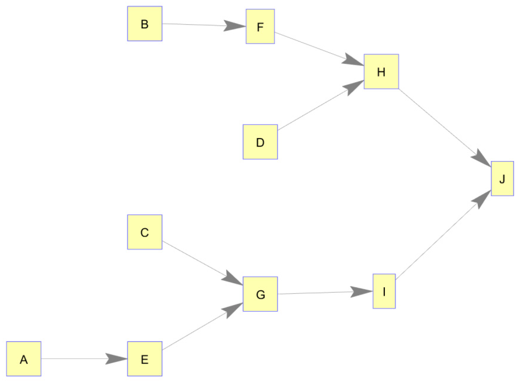
In preparation to analyze CASNs using information-theoretic principles, the authors first devised a conceptual information supply network structure and then simulated knowledge production timing schema as behaviors of each of the nodes. The conceptual network structure consisted of 10 nodes (4 source nodes, 5 intermediary nodes, and 1 final production node), as shown in
Figure 1. A simple tree structure was chosen for this case, although other structures would have been equally suitable. The methodology does not necessitate any specific number of source nodes, intermediary nodes, or final destination nodes. In fact, when applied in practice, these labels are not applied, and the methodology detects the network structure as present.
For the production schema on this network, the output of one node became an input to a second node which produced its own output based on input(s) received. All nodes’ knowledge production was governed by a simple 1-unit time delay. Essentially, a node produced information and passed it to the next node which used that for its own production 1 time unit later. In the cases in which a node had dual input sources, that node produced knowledge based on both input nodes’ information; if either source node produced information, that node also produced 1 time unit later. In the cases of the source nodes (those without any inputs), production timing was simulated as a random series with approximately 30% production frequency.
Many alternative information production timing schema could have been simulated. For example, the authors could have chosen to vary the time delays among the nodes, create randomly variable (but bounded) time delays, or to ignore some number of inputs to determine production timing [
38]. However, for this initial application, the deterministic approach of a 1-unit time delay was chosen to more clearly demonstrate the method without adding unnecessary noise.
It should be noted, that although these data are simulated, real-world data may already exist for many business applications and be readily available from workflow management software such as those discussed in Van der Aalst et al. These workflow process mining techniques address a similar problem of discovering a business process from event logs, but the method is an application of Petri nets and has limitations as to the network structures that can be discovered [
39]. It would be an interesting area of future research to compare the workflow mining techniques from those authors to the information theoretic methodologies presented here.
To complete the analysis, the authors used these simulated production times to calculate the transfer entropy for every pair of nodes in the network using the JIDT code published by Lizier [
15]. The
p-values were also calculated using the JIDT code which allows the user to compute the significance of the transfer entropy. The resulting output was then filtered to remove network links of lesser significance as determined by the
p-value. As an example, a network link could be accepted as significant if
p < 0.05, as is typical of many
p-value tests. Because this was a deterministic case, only links with
p = 0.00 were retained. In the case where uncertainty is added into the production timing data, the
p-value would need to increase accordingly.
The result of this analysis gives the user a network of nodes with significant relationships identified and weighted by transfer entropy values. As discussed previously, these transfer entropy values can be interpreted in multiple ways. Looking at relationships between individual nodes, the transfer entropy is the amount of information the source node provides about the future state of the target node (given the target’s past). This means higher transfer entropy indicates that the source node better correlates with future activity of the target. Put another way, when a source and target node pair have high transfer entropy between them, if the source node produces information, the user can reasonably expect the target node to produce information during the next time step. Additionally, transfer entropy can be viewed as the deviation from independence for two processes. Therefore, in this network example, a source and target node pair that relate with a high transfer entropy indicate that the target node is highly dependent upon information from the source node. These relationships are especially important to understand in a CASN where dependencies between nodes are continually evolving and emerging as the network adapts to its environment.
Static Network, Structure Validation
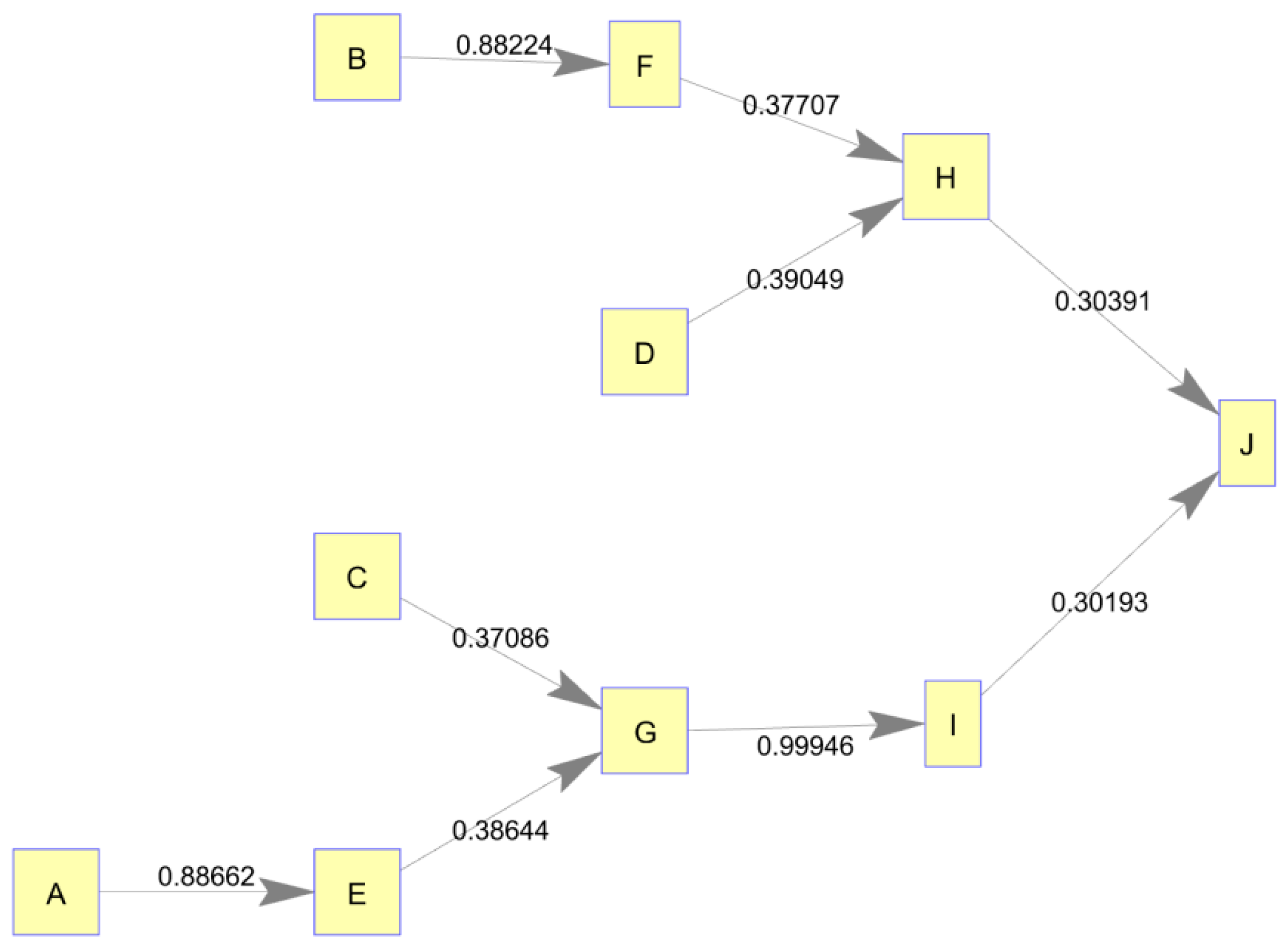
In the case of the 10-node, static supply network, transfer entropy calculations successfully uncovered the underlying conceptual network structure using only the simulated node production histories. This validated the methodologies used to simulate production dynamics within the network as well as the methodology used to analyze the static network structure. Resulting transfer entropy values and corresponding
p-values are shown in
Table 1 and
Table 2, respectively, with significant (
p = 0.00) values bolded. Because transfer entropy is a directional measure, it produces an adjacency matrix which is not symmetric enabling us to construct a directed network graph. This adjacency matrix of transfer entropy values is shown in node/edge format in
Figure 2.
2.2. Conceptual Dynamic Supply Network Simulation
The network shown in
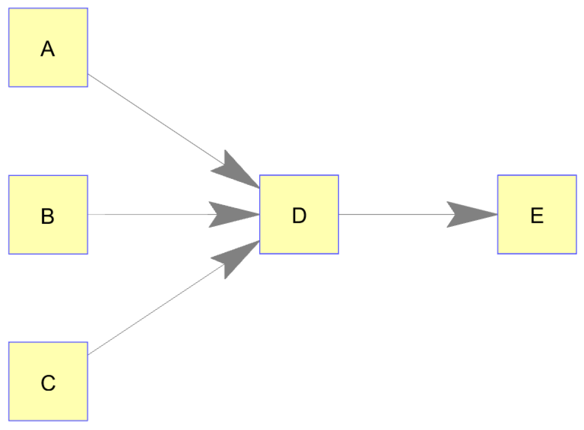
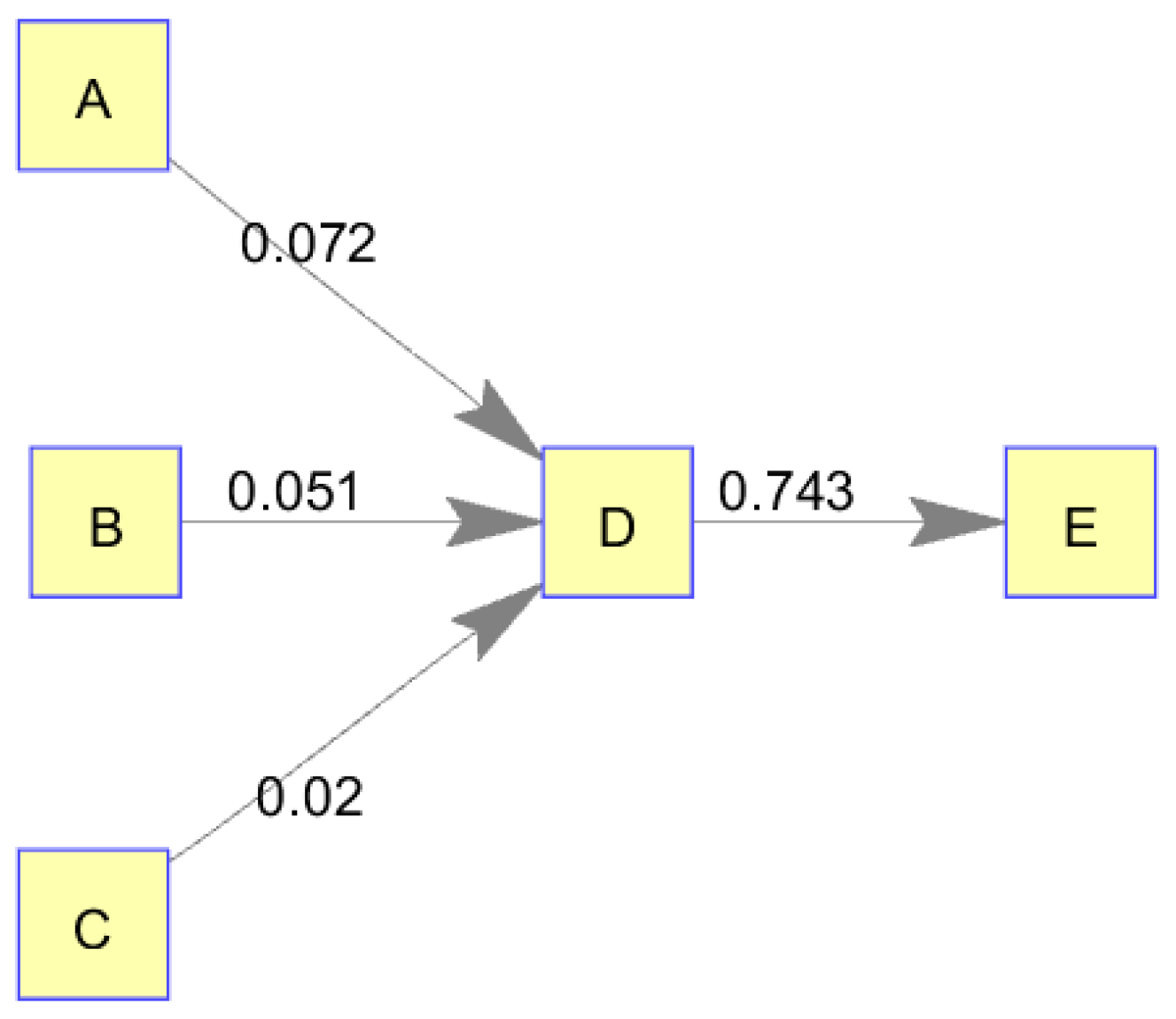
Figure 1 was considered to be static in its nodes’ dynamics; that is, the behavior of each node followed the same pattern over the entire duration of the simulation. The authors next considered a dynamic case in which a node varied which inputs it used to produce its information output. Although this was chosen as an academic case, it could represent a real-world situation in which a knowledge producer continually choses between multiple information suppliers for its production based on price, availability, et cetera. For this case, the authors created a network structure with 5 nodes (3 source nodes, 1 intermediary node, and 1 final production node), as shown in
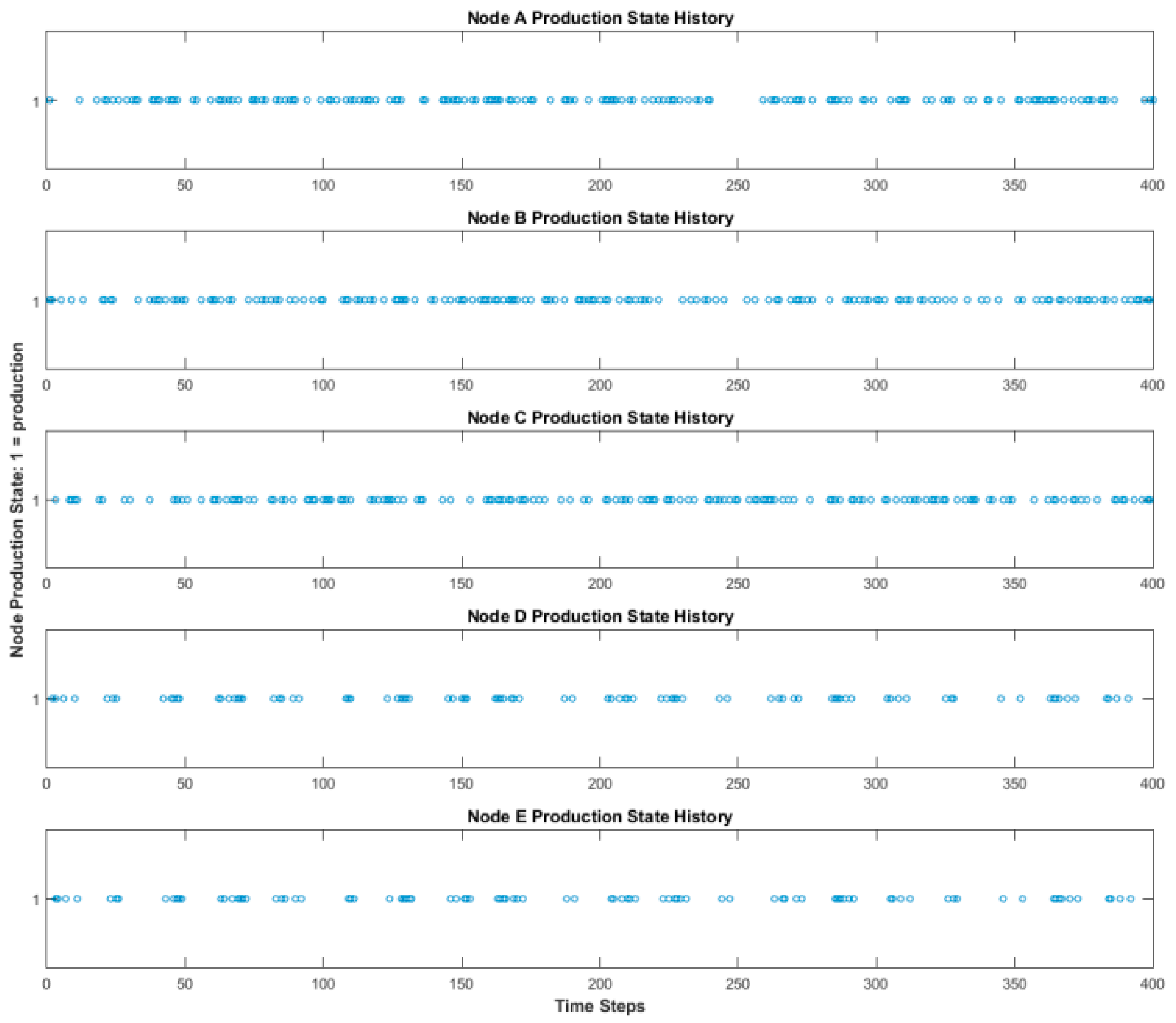
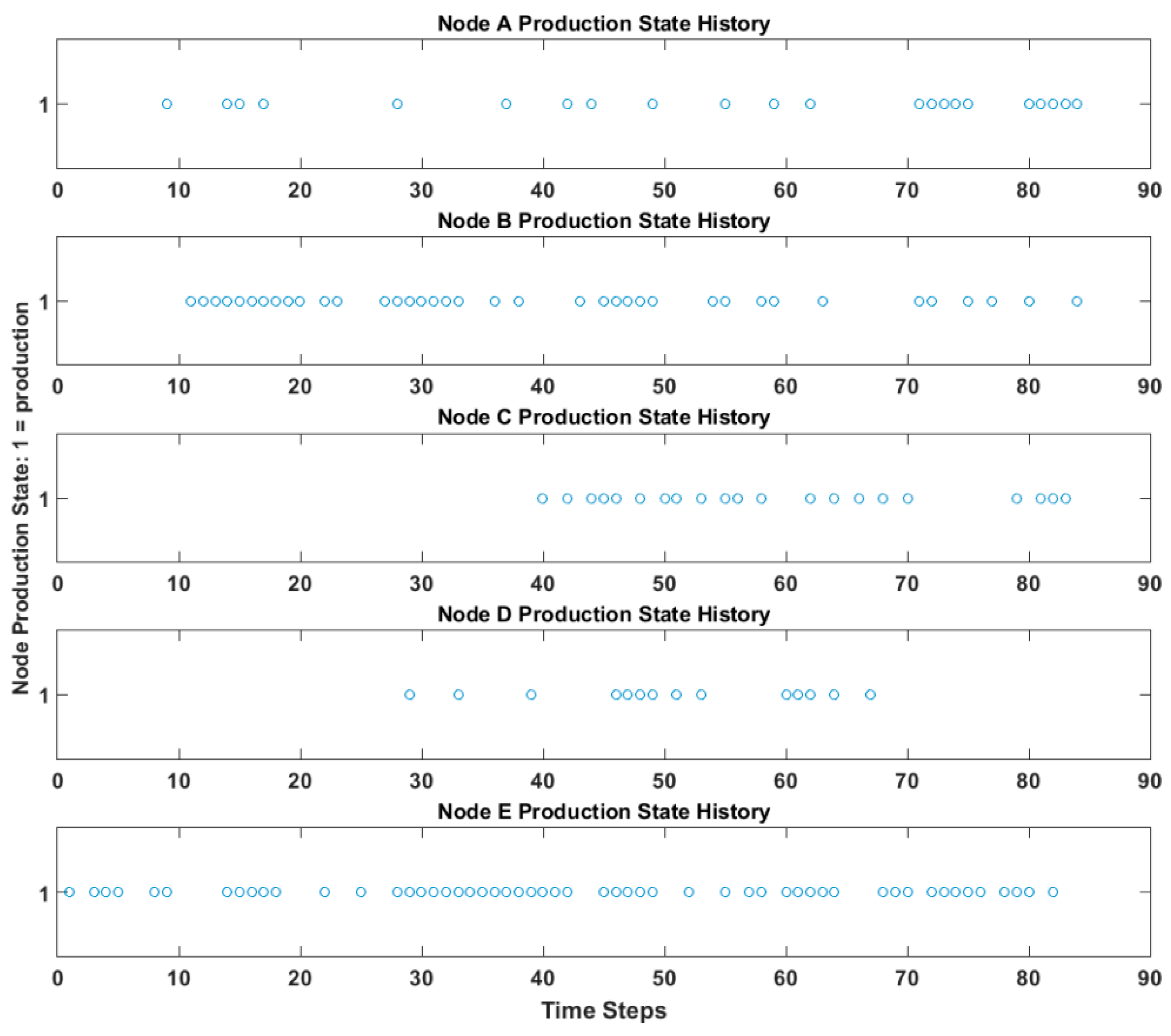
Figure 3. Here, source nodes A–C produced randomly, as before. Node E deterministically produced based on the production of node D with a 1-unit time delay. Node D, however, dynamically chose its input source from among nodes A, B, and C. In this case, node D selected a source for 20 time steps, followed by another source (or the same one) for 20 time steps, and so on. Simulated production times are shown in
Figure 4.
Using these simulated production times, the transfer entropy was calculated for every pair of nodes in the network as before. The resulting output was then filtered to remove network links of lesser significance. Only links with p < 0.001 were retained.
Additionally, using these simulated production times, the local transfer entropy was calculated using JIDT for every pair of nodes deemed to be significant. This was done to study the time-series dynamics of the nodes, especially node D which varied its relationships over time.
The result of this analysis gives the user the local transfer entropy of the relationships in the network. Again, local transfer entropy is a time history of the transfer entropy values, providing dynamic insight into the specific interactions between nodes and when they occur. The same interpretation of transfer entropy values applies to local transfer entropy analysis, except that the user now has the network relationship interactions at each time step in the time series, instead of the interaction averaged across all time steps.
2.2.1. Dynamic Network, Static Structure Validation
In the case of the dynamic supply network, transfer entropy calculations again successfully uncovered the underlying conceptual network structure using only the simulated node production histories. This validated the methodologies used to simulate production dynamics within the network as well as the methodology used to analyze the static network structure. Resulting transfer entropy values and corresponding
p-values are shown in
Table 3 and
Table 4, respectively, with significant (
p = 0.00) values bolded. This adjacency matrix of transfer entropy values is shown in node/edge format in
Figure 5.
2.2.2. Dynamic Network, Dynamic Structure Validation
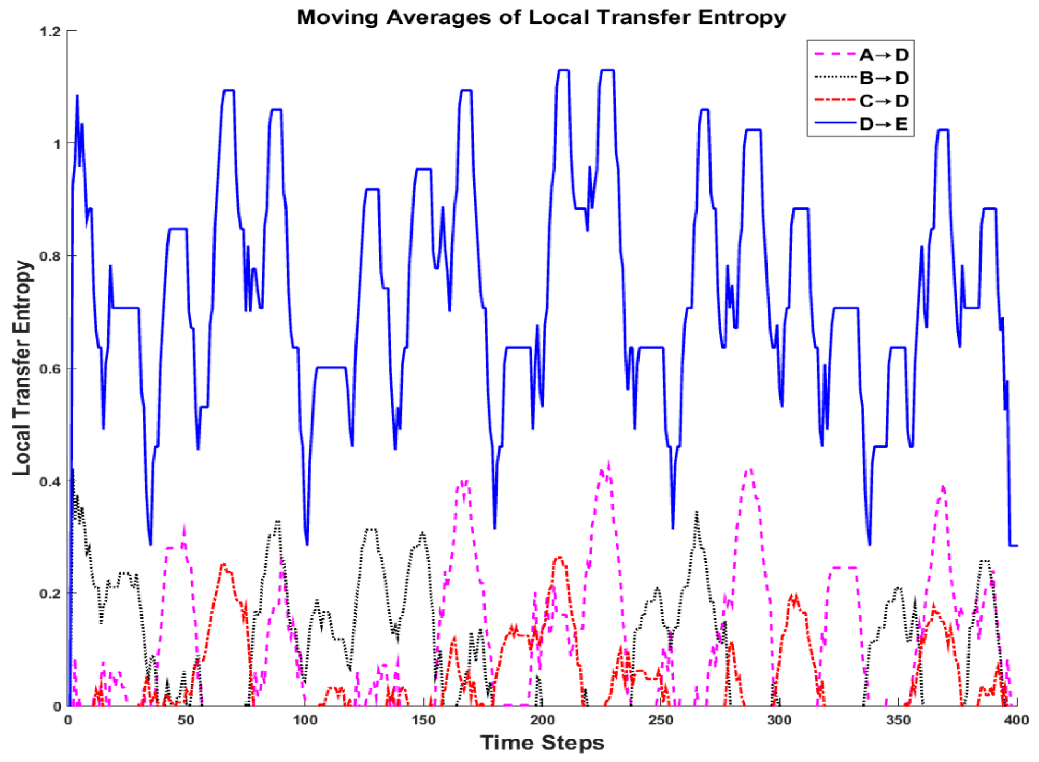
In the case of the dynamic supply network, local transfer entropy calculations again successfully uncovered the underlying conceptual network dynamics using only the simulated node production histories. This validated the methodologies used to simulate production dynamics within the network as well as the methodology used to analyze the dynamic network structure.
Because local transfer entropy can fluctuate greatly, a moving average was applied to make trends more apparent. Moving averages of 15 time units are shown in
Figure 6. This simulation was fashioned to determine whether or not changing influences in a network can be detected using information theory. Recall that node E’s production deterministically followed the production of node D. Therefore, it is intuitive that the local transfer entropy from node D→E would remain the highest of all links. Indeed, it can also be observed that this link’s average local transfer entropy is equal to the transfer entropy observed in the static network analysis between the two nodes. In addition, recall that node D selected inputs from nodes A, B, and C every 20 time steps. This is also apparent in the moving averages of local transfer entropy which display periodic behavior. By choosing
max{A→D, B→D, C→D} for each time step, it is possible to determine the source node used by node D as input in the simulation.
3. Results
3.1. Real-World, Dynamic Supply Network
Finally, these concepts were applied to a real-world network with an unknown structure. Data were obtained for an information supply network in which nodes shared information with each other in the form of knowledge production. In this real-world network, all nodes are geographically local to an organization, but nodes A–D are generally considered source nodes while node E is a hub which generally aggregates information and then passes it outside of the organization. The data for this network consisted of monthly production timing for a single topic area, as shown in
Figure 7. It should be noted that the methodology does not presume any existing relationships or labels for nodes (source, sink, etc.), but instead determines all nodes’ inputs and outputs based on their behavior. This means a node that is generally considered a source node may actually exhibit behaviors of an intermediary node in the network. This arises frequently in the context of information networks as knowledge tends to be highly collaborative. It is these differences between assumptions and real-world analysis that is of great interest to a manager of the network.
This network is similar to those information networks of news/media organizations or real-estate agencies where local sources report information to local hubs, some of which gets passed to regional hubs and then national hubs. As an example, the topic area could be likened to a real-estate topic of “single-family homes”. Each time a node (or office) created a report about a single-family home, that information was counted as production and added to the production data time-series for that node. In this situation only information about the most marketable single-family homes generated by a local office would be passed to a local hub, and then the information about the most prestigious of those homes would be passed to regional hubs.
Another parallel can be drawn here with the research area of workflow process mining. The data records available in that area of research are often tagged with information about specific tasks, specific cases, and a timestamp [
40]. The topic area of this real-world example could relate to the specific case in workflow process mining, the nodes in the network relate to the tasks in workflow logs, and the timestamp in a workflow log is captured by the time-series for that node. Again, although the authors did not choose to perform a workflow mining analysis here, the area could provide an interesting comparison for future research. It is also possible that workflow process mining tools such as EMiT (Enhanced Mining Tool) could provide alternate analyses and additional perspectives on the dataset.
Based on this production timing, the transfer entropy was calculated for every pair of nodes in the network as before to determine the underlying network structure. The resulting output was then filtered to remove network links of lesser significance. Because this real-world case contained a considerable amount of variability, links with p < 0.15 were retained. Additionally, using these simulated production times, the local transfer entropy was calculated for every pair of nodes deemed to be significant. This was done to study the time-series dynamics of the nodes to determine how their relationships varied over time.
Further, these data were then analyzed from the perspective of a manager of node E, the non-source node (or hub), which generally relies on production of the source nodes A–D. Based on all available sources, the manager was interested to learn how his organization’s dependence on those data sources had changed over the time period studied. Both transfer entropy and local transfer entropy were used to analyze node E’s dependencies, first from an average perspective and then as a dynamic time-series.
Real-World Network, Static Structure
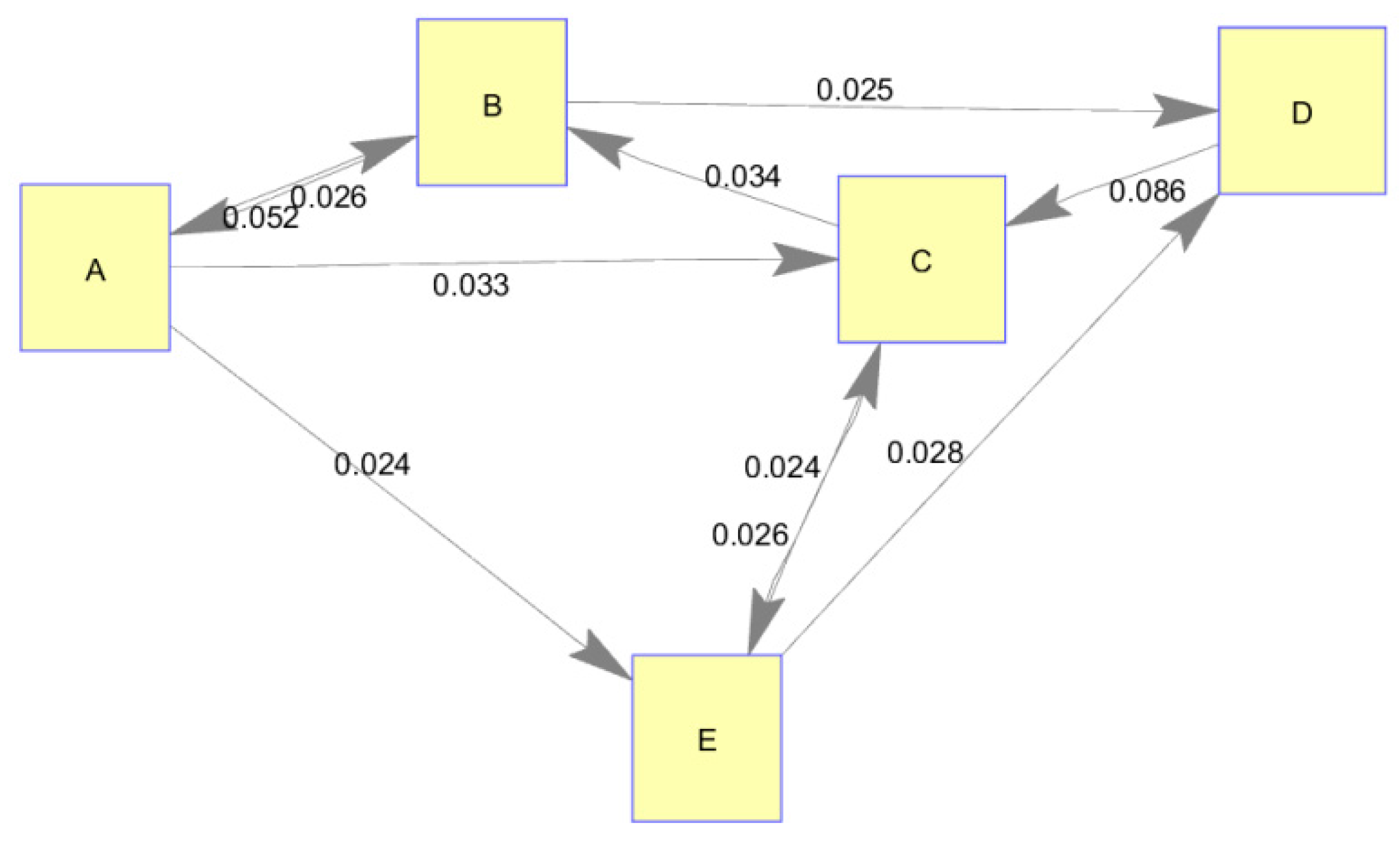
In the case of the real-world supply network, transfer entropy calculations revealed which links between network nodes were significant using only the actual node production histories. Resulting transfer entropy values and corresponding
p-values are shown in
Table 5 and
Table 6, respectively, with significant (
p < 0.15) values bolded. This
p-value was chosen in order to produce a connected graph in which every node was traversable. The adjacency matrix of transfer entropy values is shown in node/edge format in
Figure 8. Qualitative analysis of the resulting network graph shows the nodes A–D sharing significant amounts of information as this is where some of the most significant network links reside. This would appear to indicate that these nodes have a strong tendency to collaborate amongst themselves and possibly incorporate each other’s information in their production. However, these strong connections may potentially be explained by unobserved, common triggers. For example, nodes D and C may gather information from an unobserved common origin which may alternatively explain their seemingly strong link.
Because the actual information sharing network (i.e., truth data) was not known in this case, a subject matter expert on the topic area and a network manager familiar with all production offices were consulted to determine whether these new insights into the network were likely to be valid. In general, the resulting network (derived from transfer entropy) matched expectations very well for this topic area. Experts expected to see strong collaboration among nodes A–D and also expected to observe node E to be strongly dependent on nodes A and C. However, it was expected that node B would have more influence on node E’s production. It was concluded that this also made sense as information produced by node B did not typically meet a significance threshold to trigger node E’s production unless it was first combined with information from other sources.
Further, the managers noted the lack of connection between nodes A and D, which they assumed should be connected. The question arose as to whether this was an issue with processes, personnel, or some other factor. Some amount of investigation into the issue revealed poor working relationships between the individuals in nodes A and D which undoubtedly hampered collaboration. With this knowledge, the managers were able to assess paths forward to foster a connection between these offices.
These management observations highlight one of the primary characteristics of a complex adaptive system in that the agents in the network work autonomously to contribute to the overall functioning of the network. This autonomy meant the management team did not have total transparency into the inner workings of these actors without additional tools. In fact, it is these inner workings and hidden relationships that the information theoretic tools are able to discover.
Dynamic aspects of this network are considered in the next section by means of local transfer entropy.
3.2. Real-World Network, Dynamic Structure
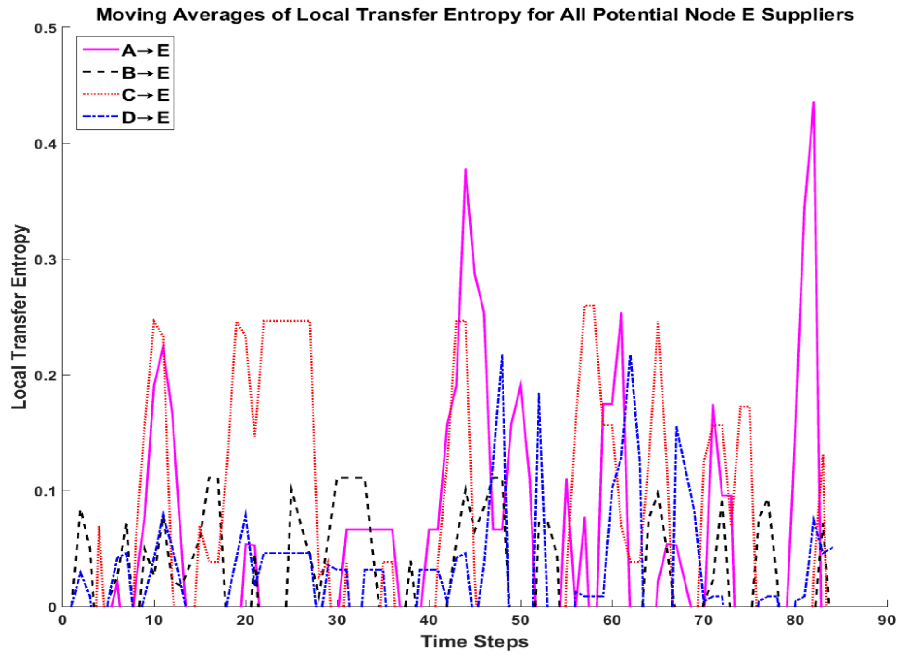
For the real-world information supply network, the next step of the methodology was to calculate the local transfer entropy for each of the links in the network. However, this time, instead of choosing all significant links as determined by the transfer entropy calculations in the static network analysis, the authors chose to evaluate the dynamics of all potential suppliers to node E. This analysis would be useful to a manager of node E to determine how the information dependencies of his organization are changing with time.
Figure 9 shows the results of the local transfer entropy calculations with a moving average of four time units applied. Again, by choosing
max{A→E, B→E, C→E, D→E} for each time step, it becomes apparent how the information dependencies of node E changed with time. Early on node E relied on significant contributions from nodes A and C, later relying heavily on node C for over 10 time units. In the second half of the time period studied, nodes A and C continued to be influential at times as well as several key spikes from node D. It is interesting to note the local transfer entropy on B→E remained low but consistent throughout this time period.
Again, no truth data were available for this network so the same subject matter expert and manager were consulted to critique these results. As before, they expected nodes A and C would be the most influential early in the time period with node C’s influence remaining high. They also expected node D would not have significance contributions until the second half of the time period at which point nodes A and C would continue with spikes of significance. As was the case with the static network analysis of this graph, it surprised the experts that node B did not have higher spikes but rather remained low throughout. This was attributed to the fact that node B does not generally produce information with enough significance to directly influence node E’s production. Instead, node B’s production was often included in the production of nodes A, C, and D upon which node E is very dependent (as evidenced by the static network structure). Overall the subject matter experts were pleased with the analysis and were excited to apply the framework to other topic areas within their organization.
4. Discussion
CASNs have challenged researchers’ ability to study them because of their dynamic nature and complex behaviors. Information theory and information dynamics provides a novel framework to overcome some of the difficulties associated with modeling CASNs. Specifically, transfer entropy can be used to determine the network structure while local transfer entropy provided insights into dynamics of those structures when applied to time-series production data.
First, the authors created a simple (10-node) conceptual supply network and simulated information production timing as a means of verifying the methodology. Transfer entropy calculations and their corresponding p-values accurately revealed the network structure based only on time-series input of the production times. Next, the authors created a dynamic conceptual supply network and again simulated production timing, also to verify the methodology. The focus of this study was to observe the local transfer entropy time series for a node which dynamically varied the inputs for its production. A static network analysis using transfer entropy and their corresponding p-values was able to uncover this network structure of significant relationships while local transfer entropy calculations determined the dynamic switching behavior of the node being studied.
Finally, a real-world information supply network with actual production time-series data was studied using this information dynamic framework. A static network analysis using transfer entropy returned a network structure which was validated by subject matter experts who have experience with the topic area and management of the real-world network. Likewise, a dynamic network analysis using local transfer entropy revealed a time-series of the changing relationships in the information sharing network. Although experts validated the analysis, the analysis also provided these managers with novel and unexpected insights into their network, especially concerning strength of relationships and relative influence between nodes in the network.
In general, managers of the network had pre-conceived notions of how their network behaved, but could not completely know how the agents in the network behaved due to the agents’ autonomy. The managers discovered they had made assumptions about how nodes communicated and passed information that may have been unfounded. This approach provided managers with new insights to an information network that they had assumed they understood and challenged the mechanisms that they assumed grounded the network. They assumed specific nodes to act as sources and specific nodes to act as sinks. However, this information theoretic methodology revealed that no nodes acted as pure source nodes and instead collaborated significantly among the other nodes. The dynamic network resulting from the methodology revealed time-history dependencies between nodes that were very close to what was expected by the managers. However, in the static structure, many relationships between the nodes surprised the managers.
Based on the static network graph produced by the methodology, the managers identified specific offices in which personnel and/or process could be fostered to increase collaboration with others. They also had assumed various relational dependencies between the nodes (which nodes’ information production could accurately predict another nodes’ information production) which did not appear significant based on these methods. Following this analysis, they had more information available in order to make resource decisions based on actual information dependencies within the network than they did based on their prior assumptions of network behavior.
These simulations and the real-world analysis showed that by using transfer entropy it is possible to reverse engineer the supply network’s structure with only time-series production data about network nodes and use local transfer entropy to analyze the network structure’s dynamics. This approach required minimal information about the network. Only node histories were needed; underlying behaviors and relationships between the nodes were not needed, modeled, or assumed. Being able to uncover network structures, either static or dynamic, from real-world data overcomes two significant barriers to studying CASN: that static and dynamic structures or underlying node behaviors must be completely known, or that node behavior must be modeled or assumed.
Furthermore, applying information theory in the context of such supply networks opens up new ways of studying these complex systems by enabling other information theoretic measures such as information storage or information modification. Other disciplines have done significant research relating information theoretic measures with network behaviors such as self-organization, emergence, stability/instability, and distributed computation, all of which remain open areas of research for CASNs. Focusing supply network research on these relationships could reveal new approaches to network management and business analytics in networks adapting to their environment.


