Sequentially Adaptive Bayesian Learning for a Nonlinear Model of the Secular and Cyclical Behavior of US Real GDP

Abstract

There is a one-to-one mapping between the conventional time series parameters of a third-order autoregression and the more interpretable parameters of secular half-life, cyclical half-life and cycle period. The latter parameterization is better suited to interpretation of results using both Bayesian and maximum likelihood methods and to expression of a substantive prior distribution using Bayesian methods. The paper demonstrates how to approach both problems using the sequentially adaptive Bayesian learning algorithm and sequentially adaptive Bayesian learning algorithm (SABL) software, which eliminates virtually of the substantial technical overhead required in conventional approaches and produces results quickly and reliably. The work utilizes methodological innovations in SABL including optimization of irregular and multimodal functions and production of the conventional maximum likelihood asymptotic variance matrix as a by-product.

1. Introduction

This paper takes up a simple but nontrivial example of a situation that arises often in econometrics. An econometric model takes the form $p\left(y\mid x,\beta \right)$ where y is a vector of outcomes, x is a vector or matrix of covariates or conditioning observables, β is an unknown parameter vector, and the functional form of p is the model specification. Due to the motivating economic theory, or by virtue of the interpretation of the model, β is a function of a more fundamental parameter vector θ, so that $\beta =\beta \left(\theta \right)$. The function need not be one-to-one. For purposes of motivation and interpretation θ is superior to β; indeed, this typically can best be accomplished in terms of θ. Examples can be found in most chapters of many econometrics textbooks, from the undergraduate to postgraduate levels. A generic case is the one in which θ expresses the underlying taste and/or technology state of a market or economy: neoclassical models of production and consumption and structural simultaneous equation macroeconometric models are two broad subcategories. The same is true in nonstructural settings like the many specific variants of linear state space models and factor models. And it is also true in the effort to provide economic interpretation of simple descriptive models like the one used here.

For a subjective Bayesian, this point has added force because a prior distribution that is substantive (by implication proper) must be expressed in terms of θ, not β. Bayesian econometrics now has a set of tools to address these nonlinear models, the most widely applied perhaps being Markov chain Monte Carlo (MCMC). This paper adds to this collection of tools the sequentially adaptive Bayesian learning algorithm (SABL). Given that there already exist multiple approaches, the question of why an additional approach naturally arises. There are several good answers to this question. The objective of this paper is to substantiate the answers, by both presenting the method and by illustrating its application to nonlinear models.

• SABL provides a generic and robust approach to the nonlinear model problem as just stated. Compared with existing methods like MCMC it requires very little tuning and experimentation with the exact form of the algorithm (for example, specification of the variance matrix for the Metropolis random walk, burn-in and convergence decisions). In many cases, like the illustration here, no tuning or experimentation at all is required.
• With a simple change of a single parameter, the SABL algorithm can be used for optimization as well as Bayesian inference. Here, that feature is used to compute maximum likelihood estimates and their associated asymptotic distribution. More generally, SABL can be used to attack a wide variety of optimization problems in economics.
• SABL enables Bayesians to use almost any prior distribution and to modify conventional distribution by imposing constraints (illustrated here) or mixing with discrete distributions (not illustrated). It also provides numerical standard errors and accurate log marginal likelihood (marginal data density) approximations as by-products, neither of which is a focus of this paper.
• In many cases SABL is faster and more accurate than any competing algorithm when executed in a conventional multicore CPU environment. That is the case for the illustration here.
• The SABL algorithm is pleasingly parallel, and except for a computationally insignificant portion of the algorithm it is embarrassingly parallel. It is therefore well suited to execution on graphics processing units, and this facility is included in SABL.

This list is not intended to be exhaustive, but rather as motivation for the reader already steeped in Bayesian computational techniques to continue on.

The paper proceeds by introducing the nonlinear model used as a simple but realistic example, Section 2. Section 3 then provides an overview of SABL used for Bayesian inference, drawing on more extensive documentation for SABL that is readily available [1]. This is followed by the illustrative example for Bayesian inference, Section 4. Section 5 takes up optimization in SABL, with a specific focus on maximum likelihood, and the illustration follows in Section 6. There is a short concluding section.

The paper is written to convey an understanding of SABL and its application to the problem set forth in the next section. For full development of the immediate theory, refer to [2,3,4]. For the underlying probability theory the single best self-contained reference is [5].

2. Interpretation of the Third-Order Autoregression

The relationship of second-order stochastic difference equations to business cycle dynamics has been recognized at least since [6]. In a model like

$$y_t={\gamma }_0+{\gamma }_1{y}_{t-1}+{\gamma }_2{y}_{t-2}+{\epsilon }_t,$$

where ${\epsilon }_t$ is the innovation (shock) for the stationary time series $\left\{y_t\right\}$, the associated characteristic polynomial is $\gamma \left(z\right)=1-{\gamma }_{1}z-\gamma z^2$. Let the roots of the polynomial be $r_1$ and $r_2$. Stationarity is equivalent to $\left|r_1\right|>1$, $\left|r_2\right|>1$. If, in addition, $r_1$ and $r_2$ are a complex conjugate pair then the time series exhibits characteristic cycles in which the amplitude is $\alpha ={\left|r_1\right|}^{-1}={\left|r_2\right|}^{-1}$ and the period is $2\pi /{tan}^{-1}\left(Im\left(r_1\right)/Re\left(r_1\right)\right)$ where ${tan}^{-1}$ denotes the principle branch in $\left(0,\pi \right)$. This is the technical essence of [6] and now a standard part of graduate education.

Geweke [7] applied a similar interpretation to the third-order stochastic difference equation (autogregression)

$$y_t={\beta }_0+{\beta }_1{y}_{t-1}+{\beta }_2{y}_{t-2}+{\beta }_3{y}_{t-3}+{\epsilon }_t,{\epsilon }_t\stackrel{iid}{\sim }N\left(0,{\sigma }^2\right),$$

(1)

taking up the case with one real root $r_1$ and a pair of complex conjugate roots $r_2$ and $r_3$ in the associated characteristic polynomial. That paper used the reparameterization

$${\alpha }_s={\left|r_1\right|}^{-1},{\alpha }_c={\left|r_2\right|}^{-1},p=2\pi /{tan}^{-1}\left(\text{Im}\left(r_2\right)/\text{Re}\left(r_2\right)\right),$$

(2)

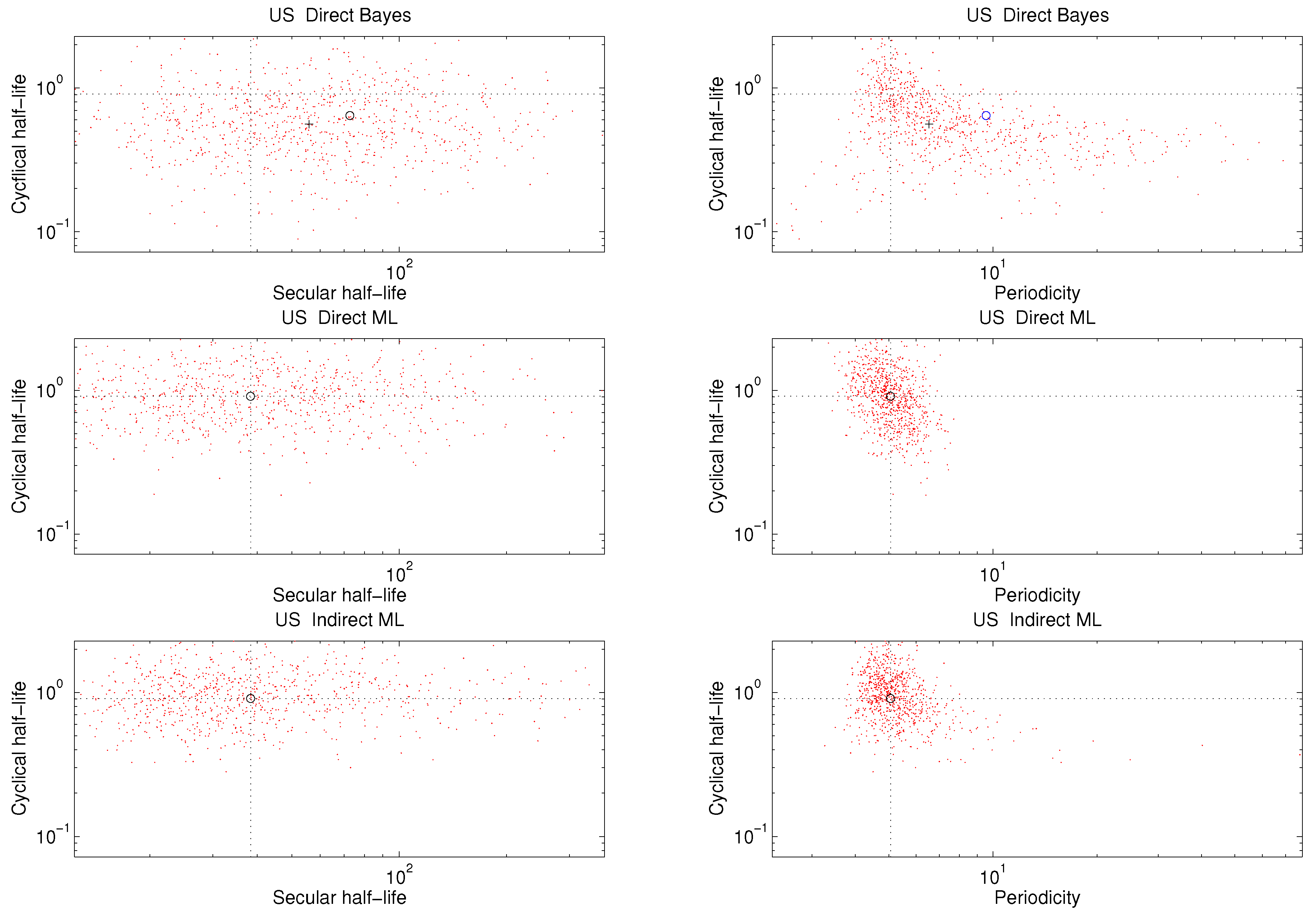
where the subscript s denotes “secular” and $c$denotes “cyclical.” It continued to impose ${\alpha }_c<1$, permitted ${\alpha }_s>1$, ${\alpha }_s-1$ then being the explosive growth rate, as well as ${\alpha }_s<1$, the rate of dampening in the transmission of ${\epsilon }_t$. The paper used a conventional improper prior distribution for β and ${\sigma }^2=\mathrm{var}\left({\epsilon }_t\right)$ and data from 19 OECD countries 1957–1983. It found posterior probabilities of explosive roots near 0, probabilities of complex pairs exceeding one-half for all countries, and probabilities that $\left|a_s\right|>\left|{\alpha }_c\right|$ over one-half for most countries.

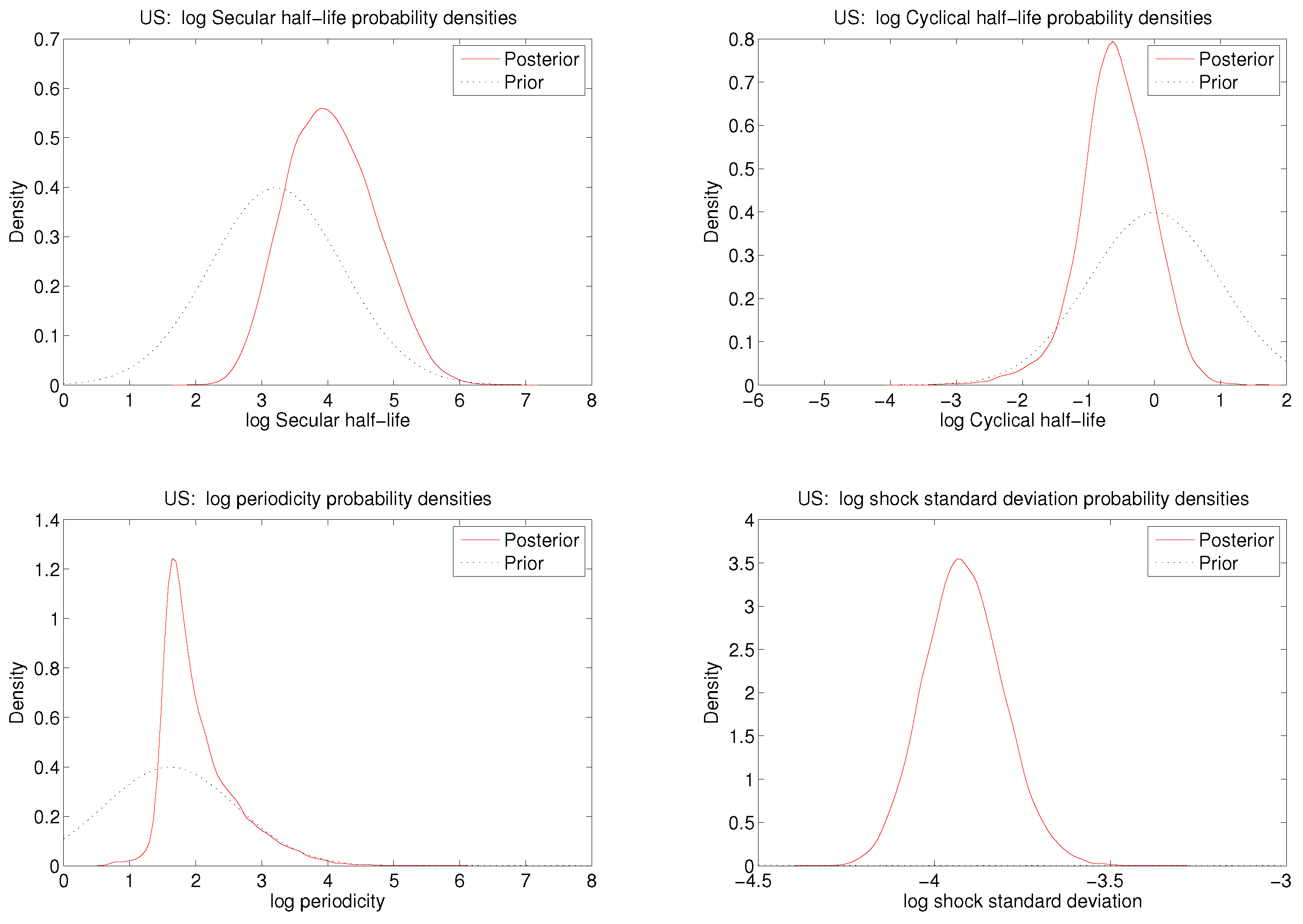
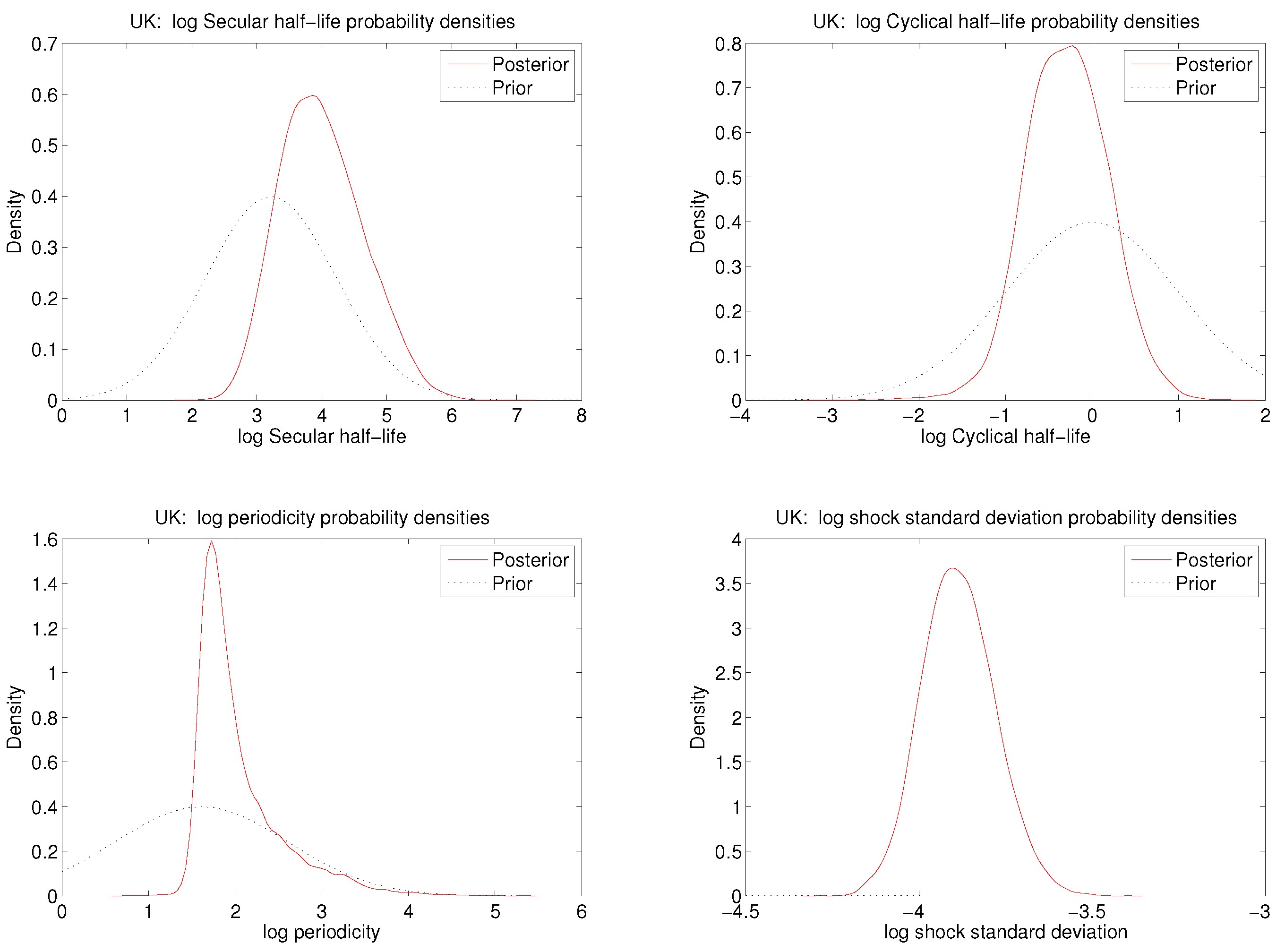
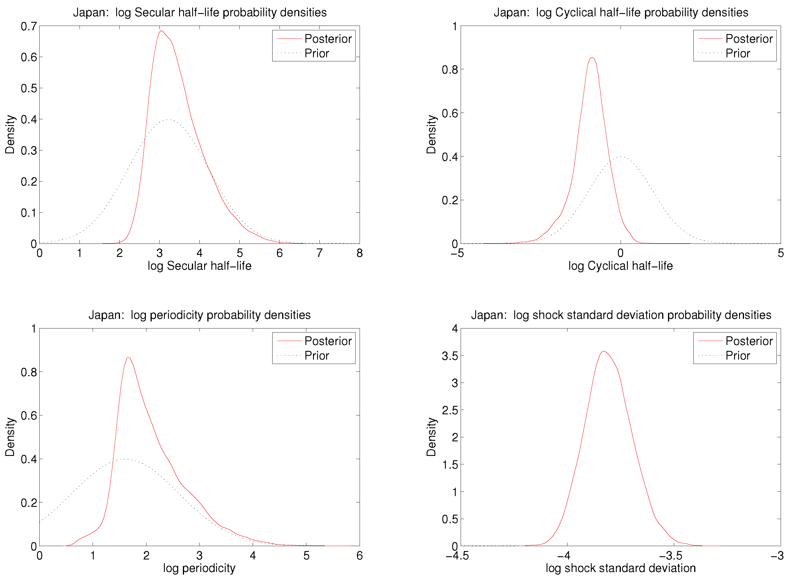
The application here works directly with parameters that are much closer to the way that economists think about growth and business cycles than are the time series parameters $\beta ={\left({\beta }_0,{\beta }_1,{\beta }_2,{\beta }_3\right)}^{\prime }$ and σ. This enables the economist to construct a substantive prior distribution and to readily understand the posterior distribution.

The work begins by replacing the amplitudes ${\alpha }_s$ and ${\alpha }_c$ with their corresponding half-lives. A damping amplitude $\alpha \in \left(0,1\right)$ generates the sequence $1,\alpha ,{\alpha }^2,\dots$, equivalent to the impulse response function in the first-order autoregression $x_t=\alpha x_{t-1}+{\eta }_t$. The corresponding half-life is the value h for which

$$\frac{{\int }_0^h{\alpha }^{u}du}{{\int }_0^{\infty }{\alpha }^{u}du}=\frac{1}{2},$$

which implies $h=log\left(1/2\right)/log\left(\alpha \right)$. Thus for the secular and cyclical components we have the inverse relations

$${\alpha }_s={\left(1/2\right)}^{1/h_s},{\alpha }_c={\left(1/2\right)}^{1/h_c}$$

(3)

mapping the secular half-life $h_s$ to its amplitude ${\alpha }_s$ and the cyclical half-life $h_c$ to its amplitude ${\alpha }_c$. Writing the generating polynomial for the stochastic difference equation (1)

$$1-{\beta }_{1}z-{\beta }_2{z}^2-{\beta }_3{z}^3=\left(1-r_{1}z\right)\left(1-r_{2}z\right)\left(1-r_{3}z\right)$$

with $r_3={\overline{r}}_2$, we obtain from (2)

$${\beta }_1={\alpha }_s+2{\alpha }_{c}cos\left(2\pi /p\right),{\beta }_2=-\left({\alpha }_s{\alpha }_c\right)cos\left(2\pi /p\right)+{\alpha }_c^2,{\beta }_3={\alpha }_s{\alpha }_c^2.$$

(4)

The domains of ${\alpha }_s$ and ${\alpha }_c$ are $\left(0,\infty \right)$. The domain of p is $\left(2,\infty \right)$, the lower bound corresponding to using the principal branch of the function ${tan}^{-1}$ in $\left(0,\pi \right)$ in (2). More fundamentally, there is an identification problem presented by aliasing: in any time series with one time unit between observations periodicities $p/\left(1+pj\right)$ $\left(j=0,1,2,\dots \right)$ all exhibit as period p. A conventional way to resolve this problem is to require $p>2$, which also seems satisfactory for business cycles with annual data.

Thus, given the half-lives $h_s$ and $h_c$ and the period p, (3) followed by (4) provides ${\beta }_1,{\beta }_2,{\beta }_3$. The mapping is continuous and has continuous derivatives of all orders. The other parameters of the model are σ, which has straightforward economic interpretation, and ${\beta }_0$, which does not but is of little interest.

It is natural to express independent prior distributions for $h_s$, $h_c$, p, and σ: most economists could readily state some plausible and some implausible values for each—unlike the case with ${\beta }_1$, ${\beta }_2$ and ${\beta }_3$. The half-lives and periods are all measured in time units and the supports of the respective prior distributions must each be (a subset of) the positive half-line. Several well-known prior distributions qualify and can easily be used in the approach taken here. We will use a log-normal prior distribution for each, the distribution for $log\left(p\right)$ being truncated below at $log2$. There are also several well-known prior distributions for σ; we again use a log normal prior. Finally, ${\beta }_0$ will be given a diffuse normal prior distribution.

Both the Bayesian approach (Section 3 and Section 4) and the maximum likelihood approach (Section 5 and Section 6) thus use the $5\times 1$ parameter vector θ with

$${\beta }_0={\theta }_1,h_s=exp\left({\theta }_2\right),h_c=exp\left({\theta }_3\right),p=exp\left({\theta }_4\right),\sigma =exp\left({\theta }_5\right)$$

The components ${\theta }_1,\dots ,{\theta }_5$ are mutually independent and normal in the prior distribution. Section 4 discusses the specific choice of the distribution. The prior distribution is also used as a computational device for maximum likelihood, but the result is unaffected by the choice of prior so long as its support includes the maximizing argument of the likelihood function. Noting that the successive transformations (2) to (3) to (4) are continuously differentiable of all orders, and considering the properties of the likelihood function for (1), it is clear that if the likelihood function has a unique internal global mode, then there is a neighborhood of the mode in which the log-likelihood function is twice continuously differentiable with bounded third derivative. This familiar condition is important to a deep verification of the properties of the SABL maximum likelihood estimates in Section 5 and Section 6.

3. Bayesian Inference Using SABL

The SABL algorithm is a procedure for the controlled introduction of new information. It pertains to situations in which information can be represented as the probability distribution of a finite dimensional vector. SABL approximates this distribution by means of many (typically on the order of ${10}^4$ to ${10}^6$) alternative versions of the vector. These versions are called particles , reflecting some of SABL’s connections to the particle filtering literature. In the SABL algorithm particles undergo a sequence of transformations as information is introduced. With minor exceptions accounting for a negligible fraction of computing time in typical research applications, these transformations amount to identical instructions that operate on each particle in isolation. SABL is therefore a pleasingly parallel algorithm. This property is responsible for dramatic decreases in computing time for many research applications with GPU execution of SABL.

At its highest level the SABL algorithm looks like this:

• Represent initial information
• While information not entirely incorporated

  -

  Determine information increment and incorporate by weighting particles

  -

  Remove the weights by resampling

  -

  Modify the particles to represent the information more efficiently

• End

In the sequential Monte Carlo literature each pass through the loop While ... End is known as a cycle, and we will use ℓ to index cycles. The three steps in each cycle are the correction (C) phase, the selection (S) phase, and the mutation (M) phase.

Let $\theta \in \Theta \subseteq {\mathbb{R}}^d$ denote the vector whose probability distribution represents information. Denote the particles by ${\theta }_{jn}$, the double subscripts indicating the J groups of N particles each employed by SABL. Initially θ has probability density $p^0\left(\theta \right)$; extension beyond absolutely continuous distributions is easy, and this streamlines the notation. In SABL the particles initially are

$${\theta }_{jn}^{\left(0\right)}\stackrel{iid}{\sim }{p}^{\left(0\right)}\left(\theta \right)\left(j=1,\dots ,J;n=1,\dots ,N\right).$$

(5)

In Bayesian inference $p^{\left(0\right)}\left(\theta \right)$ is a proper prior density and in optimization it is the probability density. It must be practical to sample from the initial distribution (5) and to evaluate $p^{\left(0\right)}\left(\theta \right)$.

Denote the density incorporating all the information by $p^{*}\left(\theta \right)$. SABL requires that it be possible to evaluate a kernel $k\left(\theta \right)$ with the properties

$$k\left(\theta \right)\ge 0\forall \theta \in \Theta ,{\int }_{\Theta }k\left(\theta \right)d\theta <\infty ,p^{*}\left(\theta \right)\propto k^{*}\left(\theta \right)=p^{\left(0\right)}\left(\theta \right)k\left(\theta \right).$$

(6)

In Bayesian inference the kernel $k\left(\theta \right)$ is the likelihood function,

$$k\left(\theta \right)=p\left(y_{1:T}\mid \theta \right),$$

(7)

where T denotes sample size and $y_{1:T}$ $=\left\{y_1,\dots ,y_T\right\}$ denotes the data.

Cycle ℓ begins with the kernel $k^{\left(\ell -1\right)}$ and ends with the kernel $k^{\left(\ell \right)}$. In the first and last cycles,

$$k^{\left(0\right)}=1\text{and}{k}^{\left(L\right)}\left(\theta \right)=k\left(\theta \right),$$

respectively. Correspondingly define

$$k^{*\left(\ell \right)}\left(\theta \right)=p^{\left(0\right)}\left(\theta \right)k^{\left(\ell \right)}\left(\theta \right),$$

(8)

implying

$$k^{*\left(0\right)}=p^{\left(0\right)}\left(\theta \right)\text{and}{k}^{*\left(L\right)}\left(\theta \right)=k^{*}\left(\theta \right).$$

(9)

The particles change in each cycle, and reflecting this let ${\theta }_{jn}^{\left(\ell \right)}$ denote the particles at the end of cycle ℓ. The initial particles ${\theta }_{jn}^{\left(0\right)}$ have the common distribution (5) and are independent. In succeeding cycles the particles ${\theta }_{jn}^{\left(\ell \right)}$ continue to be identically distributed but they are not independent. The theory underlying SABL, discussed further in this section and developed in detail by [3,4] drawing on sequential Monte Carlo theory, assures that the final particles ${\theta }_{jn}={\theta }_{jn}^{\left(L\right)}\stackrel{d}{⟶}{p}^{*}\left(\theta \right)$. This convergence in distribution takes place in N, the number of particles per group. The result is actually stronger: the particles are ergodic in N, meaning that for any function g for which $E\left[g\left(\theta \right)\right]={\int }_{\Theta }$ $g\left(\theta \right)p^{*}\left(\theta \right)d\theta$ exists,

$$\underset{N\to \infty }{lim}{N}^{-1}\sum _{n=1}^{N}g\left({\theta }_{jn}\right)=E\left[g\left(\theta \right)\right]$$

(10)

with probability 1 in each group $j=1,\dots ,J$.

A leading technical challenge in practical sequential Monte Carlo algorithms, which of course work with finite N, is to limit the dependence amongst particles, and in particular to keep dependence from increasing from one cycle to the next to the point that the final distribution of particles is an unreliable representation of any distribution at all. A further technical challenge is to provide a measure of the accuracy of the approximation implicit in the left side of (10) for finite N that is itself reliable. The SABL algorithm and toolbox do both in a way that makes minimal demands on users. The remainder of this section provides some details.

3.1. C phase

For each cycle ℓ define the weight function

$$w^{\left(\ell \right)}\left(\theta \right)=k^{\left(\ell \right)}\left(\theta \right)/k^{\left(\ell -1\right)}\left(\theta \right).$$

The theory underlying the SABL algorithm requires that there exist an upper bound ${\overline{w}}^{\left(\ell \right)}$, that is,

$$w^{\left(\ell \right)}\left(\theta \right)<{\overline{w}}^{\left(\ell \right)}<\infty \forall \theta \in \Theta .$$

The C phase determines $w^{\left(\ell \right)}\left(\theta \right)$ explicitly and thereby defines

$$k^{\left(\ell \right)}\left(\theta \right)=w^{\left(\ell \right)}\left(\theta \right)·k^{\left(\ell -1\right)}\left(\theta \right)$$

(11)

and

$$p^{*\left(\ell \right)}\left(\theta \right)=k^{*\left(\ell \right)}\left(\theta \right)d\theta /{\int }_{\Theta }{k}^{*\left(\ell \right)}\left(\theta \right)d\theta .$$

Thus (8) and (11) imply $k^{*\left(\ell \right)}\left(\theta \right)=w^{\left(\ell \right)}\left(\theta \right)·k^{*\left(\ell -1\right)}\left(\theta \right)$ as well. In SABL the weight functions $w^{\left(\ell \right)}\left(\theta \right)$ are designed so that there exists $L<\infty$ for which $k^{\left(L\right)}\left(\theta \right)=k\left(\theta \right)$, although the value of L is in general not known at the outset.

One approach in designing the weight function is to use the functional form $w^{\left(\ell \right)}\left(\theta \right)=k{\left(\theta \right)}^{{\Delta }_{\ell }}$ and determine a sequence of positive increments $\left\{{\Delta }_{\ell }\right\}$ with ${\sum }_{\ell =1}^L{\Delta }_{\ell }=1$. Thus at the end of cycle ℓ, $k^{\left(\ell \right)}\left(\theta \right)=k{\left(\theta \right)}^{r_{\ell }}$ where $r_{\ell }={\sum }_{s=1}^{\ell }{\Delta }_s$. This variant of the C phase is known as power tempering . The term originates in the simulated annealing literature in which $T_{\ell }=r_{\ell }^{-1}$ is known as temperature and $\left\{T_{\ell }\right\}$ as the cooling schedule. Another approach originates in particle filtering and Bayesian inference: $k^{\left(\ell \right)}\left(\theta \right)=p\left(y_{1:t_{\ell }}\mid \theta \right)$, where $0<t_1\dots <t_L=T$ for a sample of size T. The increments are therefore $w^{\left(\ell \right)}\left(\theta \right)=p\left(y_{t_{\ell -1}+1:t_{\ell }}\mid y_{1:t_{\ell -1}},\theta \right)$. This variant of the C phase is known as data tempering.

The C phase can be motivated informally by analogy to importance sampling, a long-established Monte Carlo simulation method, interpreting $k^{*\left(\ell -1\right)}\left(\theta \right)$ as the kernel of the source density and $k^{*\left(\ell \right)}\left(\theta \right)$ as the kernel of the target density. If it were the case that the particles ${\theta }_{jn}^{\left(\ell -1\right)}$ were independent and had common distribution indicated by the kernel density $k^{*\left(\ell -1\right)}\left(\theta \right)$, then

$$\begin{array}{ccc}& & \frac{{\sum }_{j=1}^J{\sum }_{n=1}^{N}w\left({\theta }_{jn}^{\left(\ell -1\right)}\right)g\left({\theta }_{jn}^{\left(\ell -1\right)}\right)}{{\sum }_{j=1}^J{\sum }_{n=1}^{N}w\left({\theta }_{jn}^{\left(\ell -1\right)}\right)}\stackrel{a.s.}{⟶}\frac{{\int }_{\Theta }{k}^{*\left(\ell \right)}\left(\theta \right)g\left(\theta \right)d\theta }{{\int }_{\Theta }{k}^{*\left(\ell \right)}\left(\theta \right)d\theta }\hfill \\ & =& {\int }_{\Theta }{p}^{*\left(\ell \right)}\left(\theta \right)g\left(\theta \right)d\theta =E^{\left(\ell \right)}\left[g\left(\theta \right)\right]\hfill \end{array}$$

(12)

so long as $E^{\left(\ell \right)}\left[g\left(\theta \right)\right]$ exists. The convergence is in N, the number of particles per group.

The core of the argument for importance sampling is

$${\int }_{\Theta }{p}^{*\left(\ell \right)}\left(\theta \right)g\left(\theta \right)d\theta =\frac{{\int }_{\Theta }{w}^{\left(\ell \right)}\left(\theta \right)k^{*\left(\ell -1\right)}\left(\theta \right)g\left(\theta \right)d\theta }{{\int }_{\Theta }{w}^{\left(\ell \right)}\left(\theta \right)k^{*\left(\ell -1\right)}\left(\theta \right)d\theta }=\frac{{\int }_{\Theta }{w}^{\left(\ell \right)}\left(\theta \right)p^{*\left(\ell -1\right)}g\left(\theta \right)d\theta }{{\int }_{\Theta }{w}^{\left(\ell \right)}\left(\theta \right)p^{*\left(\ell -1\right)}\left(\theta \right)d\theta }.$$

This result does not apply strictly, here, because while the particles ${\theta }_{jn}^{\left(\ell -1\right)}$ are identically distributed, they are not independent and $k^{*\left(\ell -1\right)}\left(\theta \right)$ is at best an approximation of the kernel density of the true common distribution of the particles ${\theta }_{jn}^{\left(\ell -1\right)}$ so long as $N<\infty$ (as it must be in practice). But many of the practical concerns in importance sampling carry over. In particular, success lies in $w\left(\theta \right)$ being “well-conditioned”–loosely speaking, variation in $w\left({\theta }_{jn}\right)$ must not be too great. For example, difficulties arise when just a few weights $w\left({\theta }_{jn}\right)$ account for most of the sum. In this case the target density kernel $k^{*\left(\ell \right)}\left(\theta \right)$ is represented almost entirely by a small number of particles and the approximation of $E^{\left(\ell \right)}\left[g\left(\theta \right)\right]$ implicit in the left side of (12) is poor.

The C phase directly confronts the key question of how much information to introduce in cycle ℓ: too little and L will be larger than it need be; too much, and it becomes difficult for the other phases to convert ill-weighted particles from cycle $\ell -1$ into particles from cycle ℓ sufficiently independent that the representation of the distribution does not deteriorate from one cycle to the next into a state of gross unreliability. A conventional and effective way to monitor the quality of the weight function is by means of relative effective sample size

$$RES{S}^{\left(\ell \right)}=\frac{ES{S}^{\left(\ell \right)}}{JN}=\frac{{\left[{\sum }_{j=1}^J{\sum }_{n=1}^N{w}^{\left(\ell \right)}\left({\theta }_{jn}^{\left(\ell -1\right)}\right)\right]}^2}{JN{\sum }_{j=1}^J{\sum }_{n=1}^N{w}^{\left(\ell \right)}{\left({\theta }_{jn}^{\left(\ell -1\right)}\right)}^2}.$$

(13)

The effective sample size $ES{S}^{\left(\ell \right)}$ is an adjustment to the sample size (number of particles, $JN$) that accounts for lack of balance in the weights, and relative effective size is its ratio to sample size.

In general $RES{S}^{\left(\ell \right)}$ is lower the more information is introduced in the C phase. This is always true for power tempering and as a practical matter is nearly always the case for data tempering. It suggests a strategy of introducing no further information after $RES{S}^{\left(\ell \right)}$ has attained or fallen below a target value $RES{S}^{*}$. The target $RES{S}^{*}=0.5$ is usually reasonable. Practical experience shows that somewhat higher $RES{S}^{*}$ leads to more cycles but faster execution in the M phase, lower $RES{S}^{*}$ to fewer cycles but slower M phase execution, and as a result there is not much difference in execution time over the interval $\left(0.1,0.9\right)$ for $RES{S}^{*}$.

Before any new information is introduced in the C phase $w^{\left(\ell \right)}\left(\theta \right)=1$. Data tempering entails iterations $s=1,2,\dots$ in which iteration s introduces $y_{t_{\ell -1}+s}$, updates

$$w^{\left(\ell \right)}\left({\theta }_{jn}^{\left(\ell -1\right)}\right)=w^{\left(\ell \right)}\left({\theta }_{jn}^{\left(\ell -1\right)}\right)·p\left(y_{t_{\ell -1}+s}\mid y_{t_{\ell -1}+s-1},{\theta }_{jn}^{\left(\ell -1\right)}\right),$$

and computes the corresponding $RES{S}^{\left(\ell \right)}$. Iterations terminate the first time $RES{S}^{\left(\ell \right)}<RES{S}^{*}$. This procedure is well established, though much of the sequential Monte Carlo particle filtering literature introduces exactly one new observation per cycle. In neither approach does the algorithm control the amount of information introduced in the C phase and therefore in each cycle. Indeed, routine applications of SABL demonstrate that unusual or outlying observations (e.g., asset returns for days or periods marked by financial crisis) can produce $RES{S}^{\left(\ell \right)}$ with values much smaller than $RES{S}^{*}$, imply poor performance in the S and M phases, and generally compromise the efficiency of the algorithm.

Power tempering, discussed briefly at the start of this section, makes it possible in principle for the algorithm to control the introduction of information through the choice of the sequence of increments $\left\{{\Delta }_{\ell }\right\}$. Precisely the same problem arises in simulated annealing approaches to optimization, which uses temperature, the inverse of power, and the problem is known as choice of the temperature reduction schedule. We return to this problem in Section 5, because it has some closely related aspects that apply to optimization but not Bayesian inference. The solution developed there is subsequently used for both Bayesian inference and maximum likelihood estimation in Section 4 and Section 6.

3.2. S phase

The rest of cycle ℓ starts with the weighted particles ${\theta }_{jn}^{\left(\ell -1\right)}$ from the end of the C phase and produces unweighted particles ${\theta }_{jn}^{\left(\ell \right)}$ that that meet or exceed a mixing condition—a measure of lack of dependence described in the next section—at the end of the M phase. The S phase begins this process, removing weights by means of resampling. The principle behind resampling is to regard the weight function as the kernel of a discrete probability function defined over the particles and draw from this distribution with replacement. Hence the name selection phase. SABL performs this operation on each group of particles separately—that is, particles are always selected within groups and never across groups. This independence between the groups $j=1,\dots ,J$ is essential in (1) proving the convergence of the algorithm; (2) assessing the mixing condition in the M phase; and (3) providing a numerical standard error for the approximation as discussed in Section 3.4. Resampling produces unweighted particles denoted ${\theta }_{jn}^{\left(\ell ,0\right)}$.

The most elementary resampling method is to make N independent and identically distributed draws from the multinomial distribution with argument N and probabilities

$$p_{jn}=w^{\left(\ell \right)}\left({\theta }_{jn}^{\left(\ell -1\right)}\right)/\sum _{i=1}^N{w}^{\left(\ell \right)}\left({\theta }_{ji}^{\left(\ell -1\right)}\right)\left(n=1,\dots ,N\right).$$

This method is known as multinomial resampling. An alternative method, known as residual resampling, is to compute the same probabilities and collect an initial subsample of size $N^{*}\le N$ consisting of $\left[N·p_{jn}\right]$ copies of each particle ${\theta }_{jn}$, where the function $\left[·\right]$ is standard notation for what is variously known as the greatest whole integer, greatest integer not greater than, or floor function. Then draw the remaining $N-N^{*}$ particles by means of multinomial resampling with probabilities $p_{JN}^{*}\propto N{p}_{jn}-\left[N·p_{jn}\right]$. Residual resampling results in lower dependence amongst the particles ${\theta }_{jn}^{\left(\ell ,0\right)}$ $\left(n=1,\dots ,N\right)$ than does multinomial resampling. For both methods there are central limit theorems that are essential to demonstrating convergence and interpreting numerical standard errors. There are other resampling methods that lead to even less dependence amongst the particles, but for these methods central limit theorems do not apply. These methods are all described in [5].

The S phase is a simple but key part of the SABL algorithm. Resampling is also a key part of evolutionary (or, genetic) algorithms where it plays much the same role. The particles ${\theta }_{jn}^{\left(\ell ,0\right)}$ $\left(n=1,\dots ,N\right)$ are for this reason sometimes called the children of the parent particles $\left\{{\theta }_{jn}^{\left(\ell -1\right)}\right\}$ $\left(n=1,\dots ,N\right)$, and also to emphasize the fact that for each child ${\theta }_{jn}^{\left(\ell ,0\right)}$ there is a parent ${\theta }_{j{n}^{\prime }}^{\left(\ell -1\right)}$. Parents with larger weights are likely to have more children—it is not hard to work out the exact distribution of the number of children of a given parent for any one parent for multinomial resampling and then again for residual resampling. With both, the expected number of children, or fertility, of the parent ${\theta }_{jn}^{\left(\ell -1\right)}$is proportional to $w\left({\theta }_{jn}^{\left(\ell -1\right)}\right)$, a measure of the parent’s “success” in the environment of the information introduced in cycle ℓ.

3.3. M phase

If the algorithm were to continue in this way, the number of unique children would never increase and in general would decrease from cycle to cycle. Indeed, in the context of Bayesian inference it can be shown under mild regularity conditions that the number of unique particles converges almost surely to 1 as the number of observations increases.

The M phase addresses this problem by creating diversity amongst sibling particles in a way that is faithful to the information kernel $k^{*\left(\ell \right)}\left(\theta \right)$. It does so using the same principle of invariance that is central to Markov chain Monte Carlo (MCMC) algorithms, drawing particles from a transition density $d{Q}^{\left(\ell \right)}\left(\theta \mid {\theta }^{*}\right)$ with the invariance property

$${\int }_{\Theta }{k}^{*\left(\ell \right)}\left({\theta }^{*}\right)d{Q}^{\left(\ell \right)}\left(\theta \mid {\theta }^{*}\right)d{\theta }^{*}=k^{*\left(\ell \right)}\left(\theta \right)\forall \theta \in \Theta .$$

(14)

The universe of invariant transition densities is large and manifest in the MCMC literature. Many of these transitions are model-specific, for example Gibbs sampling variants of MCMC. On the other hand a number of families of Metropolis-Hastings transitions apply quite generally and with problem-specific tuning of parameters can be computationally efficient.

SABL incorporates one of these variants, the Metropolis Gaussian random walk. The M phase applies the Metropolis random walk repeatedly in steps $s=1,2,\dots$, each step generating a new set of particles ${\theta }_{jn}^{\left(\ell ,s\right)}$ from the previous set ${\theta }_{jn}^{\left(\ell ,s-1\right)}$. Following the familiar arithmetic, candidate new particles are generated ${\theta }_{jn}^{*\left(\ell ,s\right)}\sim N\left({\theta }_{jn}^{\left(\ell ,s-1\right)},{\Sigma }^{\left(\ell ,s-1\right)}\right)$ and accepted with probability

$$min\left[\frac{k^{*\left(\ell \right)}\left({\theta }_{jn}^{*\left(\ell ,s\right)}\right)}{k^{*\left(\ell \right)}\left({\theta }_{jn}^{\left(\ell ,s-1\right)}\right)},1\right].$$

In SABL ${\Sigma }^{\left(\ell ,s\right)}$ is proportional to the sample variance of ${\theta }_{jn}^{\left(\ell ,0\right)}$ computed using all the particles. The factor of proportionality increases when the rate of candidate acceptance in the previous step exceeds a specified threshold and is decreased otherwise. This draws on established practice in MCMC and works well in this context. SABL incorporates variants of the basic Metropolis Gaussian random walk, as well, drawing on experience in the MCMC literature.

The objective of the M phase is to attain a degree of independence of the particles ${\theta }_{jn}^{\left(\ell \right)}$ at the end of each cycle sufficient to render the final set of particles ${\theta }_{jn}={\theta }_{jn}^{\left(L\right)}$ a reliable representation of the distribution implied by the probability density function $p^{*}\left(\theta \right)$. The idea behind M phase termination in SABL is to measure the degree of mixing (lack of dependence) amongst the particles at the end of each Metropolis step s of cycle ℓ, and terminate when this measure meets or exceeds a certain threshold.

In SABL mixing is measured by the average relative numerical efficiency (RNE) of a group of functions chosen specifically for this purpose in each model. The RNE of the SABL approximation of a posterior moment $E\left[g\left(\theta \right)\right]={\int }_{\Theta }g\left(\theta \right)p^{*}\left(\theta \right)d\theta$ is a measure of its numerical accuracy relative to that achieved by a hypothetical simulation ${\theta }_{ij}\stackrel{iid}{\sim }{p}^{*}\left(\theta \right)$. The next section explains how this measure is constructed. In the M phase the RNE of the particles $\left\{{\theta }^{\left(\ell ,s\right)}\right\}$ tends to increase with the number of steps s, though not monotonically.

A simple stopping rule for the M phase is to terminate the iterations of the Metropolis random walk when the average RNE of a group of functions first exceeds a stated threshold. In any application there are practical limits to the average RNE that can be achieved through these iterations, and so SABL imposes a limit on their number. Achieving greater independence of particles is especially important in the last cycle, because at the end of the M phase in that cycle the particles constitute the representation of $p^{*}\left(\theta \right)$. The SABL core default criterion is average RNE 0.4 with 100 maximum iterations in cycles $1,\dots ,L-1$ and average RNE 0.9 with 300 maximum iterations in the final cycle L.

Mixing thoroughly is not the objective of the M phase. In MCMC that is essential in providing a workable representation of the distribution with kernel $k^{*}\left(\theta \right)$. In SABL the C and S phases take on this important task, whereas the function of the M phase is to place a lower bound on the dependence amongst particles.

3.4. Convergence and the Two-Pass Variant of SABL

Durham and Geweke [3] shows that bounded likelihood and existence of the relevant prior moment together sufficient for ergodicity. In all posterior simulators the assessment of numerical accuracy is based on a central limit theorem, which in this context takes the form

$$N^{1/2}\left({\overline{g}}^{\left(J,N\right)}-\overline{g}\right)\stackrel{d}{⟶}N\left(0,{\sigma }_g^2\right)$$

(15)

where

$$\overline{g}={\int }_{\Theta }g\left(\theta \right)p^{*}\left(\theta \right)d\theta \text{and}{\overline{g}}^{\left(J,N\right)}=N^{-1}\sum _{n=1}^{N}g\left({\theta }_{jn}\right).$$

By itself (15) is not enough: it is essential to compute or approximation ${\sigma }_g^2$ as well.

The theory developed in the sequential Monte Carlo literature provides a start. It posits a fixed pre-specified sequence of kernels $k^{\left(1\right)},\dots ,k^{\left(L\right)}$ (see (11)) and a fixed pre-specified sequence of M phase transition densities $d{Q}^{\left(\ell \right)}$ (see (14)), together with side conditions (implied by bounded likelihood and the existence of prior moments), and proves (15). For example, this is the framework set up in [8] as well as the careful treatment in [5]. But in any practical application the kernels $k^{\left(\ell \right)}$ and transition densities $d{Q}^{\left(\ell \right)}$ are adaptive, relying on information in the particles ${\theta }_{jn}^{\left(\ell -1\right)}$ or ${\theta }_{jn}^{\left(\ell ,s-1\right)}$, rather than fixed. The theory does not apply then because the kernels and transitions depend on the random particles, and the structure of this dependence is so complex as to preclude extension of the existing theory to this case—especially for the transition kernels $d{Q}^{\left(\ell \right)}$. Thus, this literature provides a theory of sequential Bayesian learning but not a theory of sequentially adaptive Bayesian learning. It is universally recognized that some form of adaptation is required, for it is impossible to pre-specify kernels $k^{\left(\ell \right)}$ and transition densities $d{Q}^{\left(\ell \right)}$ that provide reliable approximations in tolerable time without knowing a great deal about the posterior distribution—which, of course, is the goal and not the starting point.

Durham and Geweke [3] deals with this issue by creating the two-pass variant of the algorithm. The first pass is exactly as described in this section, with the addition that the kernels $k^{\left(\ell \right)}$ and transitions $d{Q}^{\left(\ell \right)}$ are saved. For the specific variants described in Section 3.1 and Section 3.3, this amounts to saving the sequence $\left\{r_{\ell }\right\}$ or $\left\{t_{\ell }\right\}$ from the C phase and the doubly-indexed sequence of variance matrices ${\Sigma }^{\left(\ell ,s-1\right)}$ from the M phase, but the idea generalizes to other variants of the C and M phases. The second pass re-executes the algorithm (with different seeds for the random number generator) and uses the kernels $k^{\left(\ell \right)}$ and transitions $d{Q}^{\left(\ell \right)}$ computed in the first pass, skipping the work required to compute these objects from the particles. The theory developed in the sequential Monte Carlo literature then applies directly to the second pass, because the kernels $k^{\left(\ell \right)}$ and transitions $d{Q}^{\left(\ell \right)}$ are in fact fixed in the second pass.

Experience thus far is that substantial differences between the first and second passes do not arise, and can only be made to do so by specifying imprudently small values of N. Thus in practice it suffices to use the two-pass algorithm only occasionally—perhaps at the inception of a research project when the general character of the model(s), data and sample size are known, and then again prior to communicating findings.

The sequential Monte Carlo literature provides abstract expressions for ${\sigma }_g^2$ in (15) but no means of evaluating or approximating ${\sigma }_g^2$. SABL provides the approximation using the particle groups. Consider the second pass of the two-pass algorithm where the convergence theory fully applies. In this setting there is no dependence of particles across groups. The M phase and the C phase are perfectly parallel: exactly the same operations applied to all the particles with no communication between particles. Resampling in the S phase, which introduces dependence amongst particles, takes place entirely within groups so as not to compromise independence across groups. Therefore the approximations ${\overline{g}}_{jN}=N^{-1}{\sum }_{n=1}^{N}g\left({\theta }_{jn}\right)$ of $\overline{g}=E\left[g\left(\theta \right)\right]$ are independent across the groups $j=1,\dots ,J$. A central limit theorem (15) applies within each group so long as $g\left(\theta \right)$ has finite second moment. Computing the cross-group mean ${\overline{g}}_{J,N}=J^{-1}{\sum }_{j=1}^J{\overline{g}}_{jN}$, a conventional estimate of ${\sigma }_g^2$ in (15) is

$${\widehat{\sigma }}_g^2=N·{\left(J-1\right)}^{-1}\sum _{j=1}^J{\left({\overline{g}}_{jN}-{\overline{g}}_{J,N}\right)}^2$$

(16)

and

$$\left(J-1\right){\widehat{\sigma }}_g^2/{\sigma }_g^2\stackrel{d}{⟶}{\chi }^2\left(J-1\right),$$

(17)

the convergence in (17) being in particles per group N. In the limit $N\to \infty$, ${\overline{g}}_{J,N}$ and ${\widehat{\sigma }}_g^2$ are independent.

The corresponding numerical variance estimate for ${\overline{g}}_{J,N}$ is

$${\widehat{\sigma }}_{g,JN}^2={\left(JN\right)}^{-1}{\widehat{\sigma }}_g^2.$$

(18)

This should not be confused with the approximation of the posterior variance $\mathrm{v}\widehat{\mathrm{a}}\mathrm{r}\left(g\right)={\left(JN\right)}^{-1}{\sum }_{j=1}^J{\sum }_{n=1}^N{\left[g\left({\theta }_{jn}\right)-{\overline{g}}_{J,N}\right]}^2$. The numerical standard error corresponding to (18) is ${\widehat{\sigma }}_{g,JN}={\left[{\widehat{\sigma }}_{g,JN}^2\right]}^{1/2}$. This is the measure of accuracy used in SABL. From (17) the formal interpretation of numerical standard error is $\left({\overline{g}}_{J,N}-\overline{g}\right)/{\widehat{\sigma }}_{g,JN}\stackrel{d}{⟶}t\left(J-1\right)$. If particles within groups are independent then ${\widehat{\sigma }}_g^2\approxeq \mathrm{v}\widehat{\mathrm{a}}\mathrm{r}\left(g\right)$, whereas if they are not then usually ${\widehat{\sigma }}_g^2>\mathrm{v}\widehat{\mathrm{a}}\mathrm{r}\left(g\right)$, although ${\widehat{\sigma }}_g^2<\mathrm{v}\widehat{\mathrm{a}}\mathrm{r}\left(g\right)$ may occur and is more likely with smaller numbers of particle groups J. The relative numerical efficiency of the approximation ${\overline{g}}_{J,N}$ is

$$RN{E}_g=\mathrm{v}\widehat{\mathrm{a}}\mathrm{r}\left(g\right)/{\widehat{\sigma }}_g^2.$$

(19)

A useful interpretation of (19) is that a hypothetical simulator with ${\theta }_{jn}\stackrel{iid}{\sim }{p}^{*}\left(\theta \right)$ would achieve the same accuracy with $RN{E}_g·JN$ particles.

This argument does not apply directly in the first pass because of the adaptation. In particular, recall that RNE is used in the M phase to assess mixing and determine the end of the sequence of iterations of the Metropolis random walk. This is an example of the complex feedback between particles and adaptation in the algorithm that has frustrated central limit theorems. This shortfall in theory is likely to persist. The two-pass procedure overcomes the problem and, moreover, provides the foundation for future variants of the algorithm without the overhead of establishing convergence for each variant.

4. Posterior Distributions of Half-Lives, Periods and Shocks

With the SABL infrastructure in place drawing a posterior sample is very simple and extremely fast.

4.1. Priors and Data

The prior distributions used in the quantitative results presented here are

$$\begin{array}{ccc}\hfill \text{Parameter}& \text{Distribution}& \text{Centered 90\% interval}\hfill \\ \multicolumn{1}{c}{\text{Intercept} {\beta }_0\left(1\right):}& \multicolumn{1}{c}{{\beta }_0\sim N\left(10,5^2\right)}& \multicolumn{1}{c}{{\beta }_0\in \left(1.77,18.22\right)}\\ \multicolumn{1}{c}{\text{Secular half-life} h_s:}& \multicolumn{1}{c}{log\left(h_s\right)\sim N\left(log\left(25\right),1\right)}& \multicolumn{1}{c}{h_s\in \left(5.591,111.9\right)}\\ \multicolumn{1}{c}{\text{Cyclical half-life} h_c:}& \multicolumn{1}{c}{log\left(h_c\right)\sim N\left(log\left(1\right),1\right)}& \multicolumn{1}{c}{h_c\in \left(0.2237,22.36\right)}\\ \multicolumn{1}{c}{\text{Period} p:}& \multicolumn{1}{c}{log\left(p\right)\sim N\left(log\left(5\right),1\right),p>2}& \multicolumn{1}{c}{p\in \left(2.316,28.46\right)}\\ \multicolumn{1}{c}{\text{Shock} \sigma \left(1\right)}& \multicolumn{1}{c}{log\left(\sigma \right)\sim N\left(log0.025,1\right)}& \multicolumn{1}{c}{\sigma \in \left(0.005591,0.1118\right)}\end{array}$$

All the priors but the first are substantive, that is, grounded in consideration of what is reasonable and what is not. The standard deviation 1 for these four corresponds to change in the parameter (e.g., $h_s$) by a factor of $e=2.718$.

Given the interpretation of the parameters, I think it unlikely that an economist would claim as reasonable any values outside the stated 90% intervals. Indeed, many would be comfortable with more concentrated prior distributions. As will be seen, while the data contribute more to the posterior distributions than do the priors, the contribution of priors for half-lives and period is substantial. The effects of changing the prior hyperparameters are not hard to assess because all five parameters are nearly independent in the posterior distribution as well as in the prior.

The data used in this exercise are annual OECD per capital real GDP constant purchasing power parity [9]. Data for 26 countries are available from 1970 through 2014, so given the three lags in (1) there are 42 annual observations. We concentrate on a more detailed presentation for the US, UK and Japan rather than in drawing comparisons and conclusions for all countries.

4.2. Computation

All of the results presented here were obtained using SABL Edition 2015a [1], a Matlab toolbox that has many options including massively parallel execution on graphics processing units as well as conventional muticore CPU execution. Some options important to the work here are

• Choice of Bayesian or maximum likelihood inference, depending on a single parameter setting;
• A system for mapping fundamental parameters (here, the vector θ specified in (2)) to the parameters of the normal model (here, β and σ in (1)) using a generic mapping system that applies in all models (here, the map is given by (2)–(4));
• A system for specifying different prior distributions, either conventional or customized, for different components. In most cases there are options for truncation of prior distributions, like that for $log\left(p\right)$.

Using SABL entails writing a single Matlab function for which there are templates included in the toolbox.

Table 1. SABL output, US posterior distribution.

SABL normal model

SABL executing using CPU with 1 worker

C phase anneal_Bayes algorithm

Effective sample size criterion (C.Cstop.ress) = 0.500

C phase Cstop_unconditional algorithm

S phase residual resampling

M phase MGRW_simple algorithm

M phase Mstop_rne stopping algorithm

Simulating 16384 times from truncated prior... 2.5324 seconds

Cycle 1 Cphase: Likelihood function exponent 8.5448e-03, RESS 0.5000

Cycle 1 Sphase: 8565 particles out of 16384 unique (0.5228)

Cycle 1 Mphase: 1 iterations, mean RNE = 0.8175

Cycle 2 Cphase: Likelihood function exponent 7.1163e-02, RESS 0.5000

Cycle 2 Sphase: 7533 particles out of 16384 unique (0.4598)

Cycle 2 Mphase: 5 iterations, mean RNE = 0.4875

Cycle 3 Cphase: Likelihood function exponent 2.0704e-01, RESS 0.5000

Cycle 3 Sphase: 8374 particles out of 16384 unique (0.5111)

Cycle 3 Mphase: 1 iterations, mean RNE = 0.4208

Cycle 4 Cphase: Likelihood function exponent 4.9638e-01, RESS 0.5000

Cycle 4 Sphase: 5084 particles out of 16384 unique (0.3103)

Cycle 4 Mphase: 4 iterations, mean RNE = 0.4472

Cycle 5 Cphase: Likelihood function exponent 1.0000e+00, RESS 0.6051

Cycle 5 Sphase: 7471 particles out of 16384 unique (0.4560)

Cycle 5 Mphase: 14 iterations, mean RNE = 0.9179

Elapsed clock time 5.52 seconds

CPU time 7.71 seconds

Ratio 1.40

provides the output from the computation of the posterior distribution for the US data. It uses the same terminology as Section 3. All of the technical parameters associated with the SABL algorithm are the default values; any of them can be changed in the single function the user writes to interface with SABL. Execution with the default number of particle groups $\left(J=8\right)$ and particles per group $\left(N=1024\right)$ required less than 6 seconds on a standard laptop with a quadcore CPU. Of this, almost half the time was taken up generating the initial values from the truncated prior distribution for $log\left(p\right)$. Notice that the relative effective sample size is exactly the target value in each cycle. Each M phase continues until RNE 0.4 or greater has been achieved, but the last cycle applies the higher standard of 0.9 in order to provide more information in the final set of particles. Thus the $16,384$ particles are nearly independent. It is easy to access any posterior moment along with its numerical standard error. Log marginal likelihood is produced as a by-product.

4.3. Findings

Table 2. US posterior moments.

Parameter		Mean	st. dev.
Secular $log\left(h_s\right)$		4.056	0.667
Cyclical $log\left(h_c\right)$		−0.584	0.548
Period $log\left(p\right)$		2.045	0.565
Shock $log\left(\sigma \right)$		−3.916	0.113
Correlation matrix:
1.000	0.010	−0.021	0.001
0.101	1.000	−0.366	−0.018
−0.021	−0.366	1.000	0.022
0.001	−0.018	0.022	1.000

,

Table 3. UK posterior moments.

Parameter		Mean	st. dev.
Secular $log\left(h_s\right)$		4.002	0.655
Cyclical $log\left(h_c\right)$		−0.292	0.479
Period $log\left(p\right)$		2.041	0.502
Shock $log\left(\sigma \right)$		−3.885	0.106
Correlation matrix:
1.000	0.027	−0.034	0.022
0.027	1.000	−0.515	−0.060
−0.034	−0.515	1.000	0.078
0.022	−0.060	0.078	1.000

and

Table 4. Japan posterior moments.

Parameter		Mean	st. dev.
Secular $log\left(h_s\right)$		3.470	0.654
Cyclical $log\left(h_c\right)$		−0.951	0.543
Period $log\left(p\right)$		2.101	0.641
Shock $log\left(\sigma \right)$		−3.806	0.111
Correlation matrix:
1.000	0.030	0.084	0.133
0.030	1.000	−0.200	0.041
0.084	−0.200	1.000	−0.003
0.133	0.041	−0.003	1.000

provide the first two posterior moments of the functions of interest $log\left(h_z\right)$, $log\left(h_c\right)$, $log\left(p\right)$ and $log\left(\sigma \right)$. Two aspects of these results are striking. First, the results for the three countries are quite similar. Given the integration of the global economy in this period and the contemporaneous data, this is perhaps not surprising. Second, in each case the four parameters are nearly uncorrelated in the posterior distribution. This is in marked contrast to the situation for the parameter vector β in (1), where there is large correlation due the multicolinearity in $\left(y_{t-1},y_{-2},y_{t-3}\right)$. This supports the efficacy of working with the chosen parameterization.

Figure 1, Figure 2 and Figure 3 provide the posterior density for each parameter, computed using a standard kernel smoothing algorithm optimized for normal distributions, together with the normal prior distribution for each. (The truncation for the $log\left(p\right)$ prior is not shown.) Since all four parameters are transformed to logarithms, a common measure of the information in prior plus data is available. From Table 2, Table 3 and Table 4 and the northwest panel in each figure, over a 90% posterior credible interval secular half-life $h_s$ changes by a factor of about 12 to 15. For $h_c$ and p the range is about 8 to 9, and the factor is about 8 to 9, and for σ it is about 1.5 to 1.6. The relative confidence is not surprising: in a sample of any given length there are fewer secular fluctuations (which take many years) than there are cyclical fluctuations (which take a few years), whereas there is almost no dependence across observations in the information provided for σ.

The mechanics of how the prior distribution influences the posterior are straightforward in this situation. Since there is no correlation between parameters in the data and little in the posterior, by implication prior and data combine for each parameter with little interaction. Given the standard deviations of the prior distribution and the posterior distribution (Table 2, Table 3 and Table 4), data precision is only modestly higher than prior precision. Thus a location shift of a prior distribution by v units will produce a shift of a little less than $v/2$ units in the mean of the posterior distribution. Section 6 will compare these posterior distributions with those that would be obtained using the “diffuse” prior distribution in [7].

5. Maximum Likelihood Using SABL

With minor modification of the C phase, SABL handles global optimization problems as well as inference problems. This section provides a heuristic approach; for more formal motivation and technical details, see [2] and [4].

5.1. The Method

To begin, consider replacing the kernel $k\left(\theta \right)$ of Section 3 with the kernel $k{\left(\theta \right)}^q$ with $q>1$. The corresponding probability density is now more concentrated than it was originally. The Bayesian annealing algorithm could proceed in precisely the same way but now terminating with $r_L=q$ rather than $r_L=1$. Of course, the particles at that point would not correspond to a posterior distribution: such an interpretation would amount to an erroneous replication of the sample and additional $q-1$ times. But everything stated in Section 3 about approximation of the distribution with kernel $k\left(\theta \right)$ remains true for the distribution with kernel $k{\left(\theta \right)}^q$.

Next consider what happens as q moves to increasingly higher values, and to this end two properties of $k\left(\theta \right)$ are useful:

• The kernel $k\left(\theta \right)$ has a unique global mode ${\theta }^{*}$;
• $logk\left(\theta \right)$ is twice continuously differentiable with bounded third derivative in a neighborhood of ${\theta }^{*}$, and ${\partial }^{2}logk\left(\theta \right)/\partial \theta \partial {\theta }^{\prime }{\mid }_{\theta ={\theta }^{*}}=H$, a negative definite matrix.

In the applications in this paper $k\left(\theta \right)$ is the likelihood function and similar conditions are invoked in standard limit theorems for posterior distributions and maximum likelihood estimators. The difference is that here the limit is $q\to \infty$ rather than increasing sample size.

Recall that in cycle ℓ of the annealing variant of the SABL algorithm the exponent of $k\left(\theta \right)$ becomes $r_{\ell }$. Denote the variance matrix of particles at the end of this cycle by $V_{\ell }$.

The following four implications follow, the first from the first property and the others from both. The first three are unsurprising given conventional results for the limits of posterior distributions and maximum likelihood estimators.

• The probability distribution corresponding to the kernel $k{\left(\theta \right)}^q$ converges in distribution to the point ${\theta }^{*}$.
• The probability distribution of $q^{1/2}\left(\theta -{\theta }^{*}\right)$ converges in distribution $N\left(0,H^{-1}\right)$.
• Taking the limit first as the number of particles N increases and then as the cycle ℓ increases,

  $$r_{\ell }^{-1}{V}_{\ell }\stackrel{a.s.}{⟶}{H}^{-1},$$

  (20)

  which is the asymptotic variance of the maximum likelihood estimator.
• Taking limits in the same way, the power increase ratio ${\rho }_{\ell }=\left(r_{\ell }-r_{\ell -1}\right)/r_{\ell -1}$ converges almost surely to

  $$\rho =RES{S}^{*-2/d}-1+{\left[\left(RES{S}^{*-2/d}-1\right)·RES{S}^{*-2/d}\right]}^{1/2},$$

  (21)

  where d is the dimension of θ. Note that ρ, the asymptotic power increase ratio, depends on $k\left(\theta \right)$ only through d.

A strength of this approach is that there is no need to determine first and second derivatives, either analytically or by means of numerical differentiation. The only requirements are (a) verify properties 1 and 2 analytically, (b) derive the likelihood function, (c) code the evaluation of the log-liklelihood function, and (d) code nonlinear parameter transformations. For many applications these requirements become trivial if one is using a nonlinear parameterization of an existing model, thus avoiding (b) and (c). In particular this approach avoids analytical derivation and code testing for first or second derivatives, or numerical evaluation of derivatives, both of which can be time consuming, tedious and encounter arcane numerical problems.

The results are insensitive to the prior distribution so long as the prior distribution provides support in a neighborhood of ${\theta }^{*}$, the same condition invoked in the derivation of the asymptotic properties of posterior distributions. A practical consideration, here, is that as prior probability in this neighborhood decreases, $r_1$ becomes smaller and the number of cycles required to achieve a given concentration of particles becomes greater.

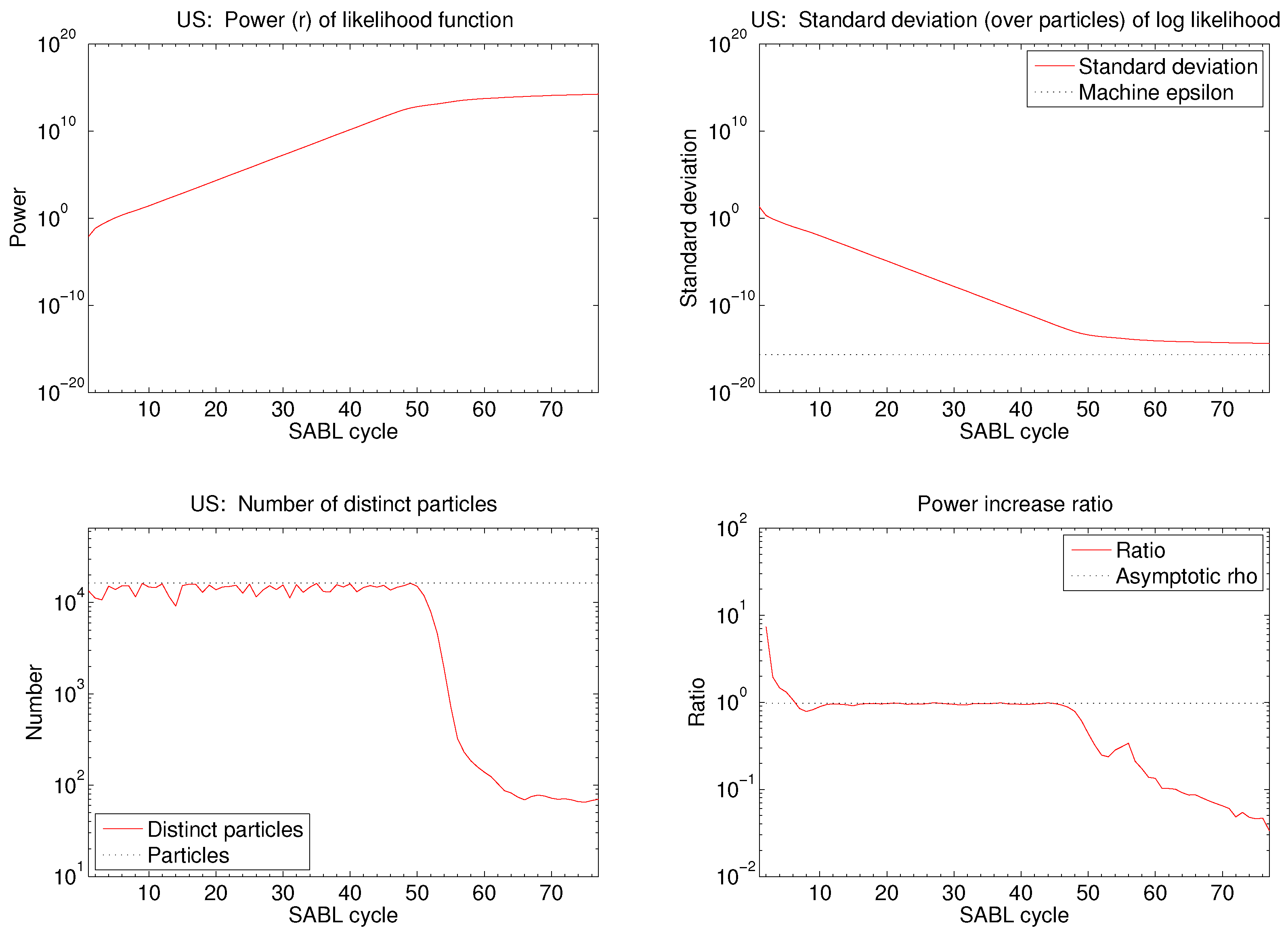
5.2. Convergence Criteria

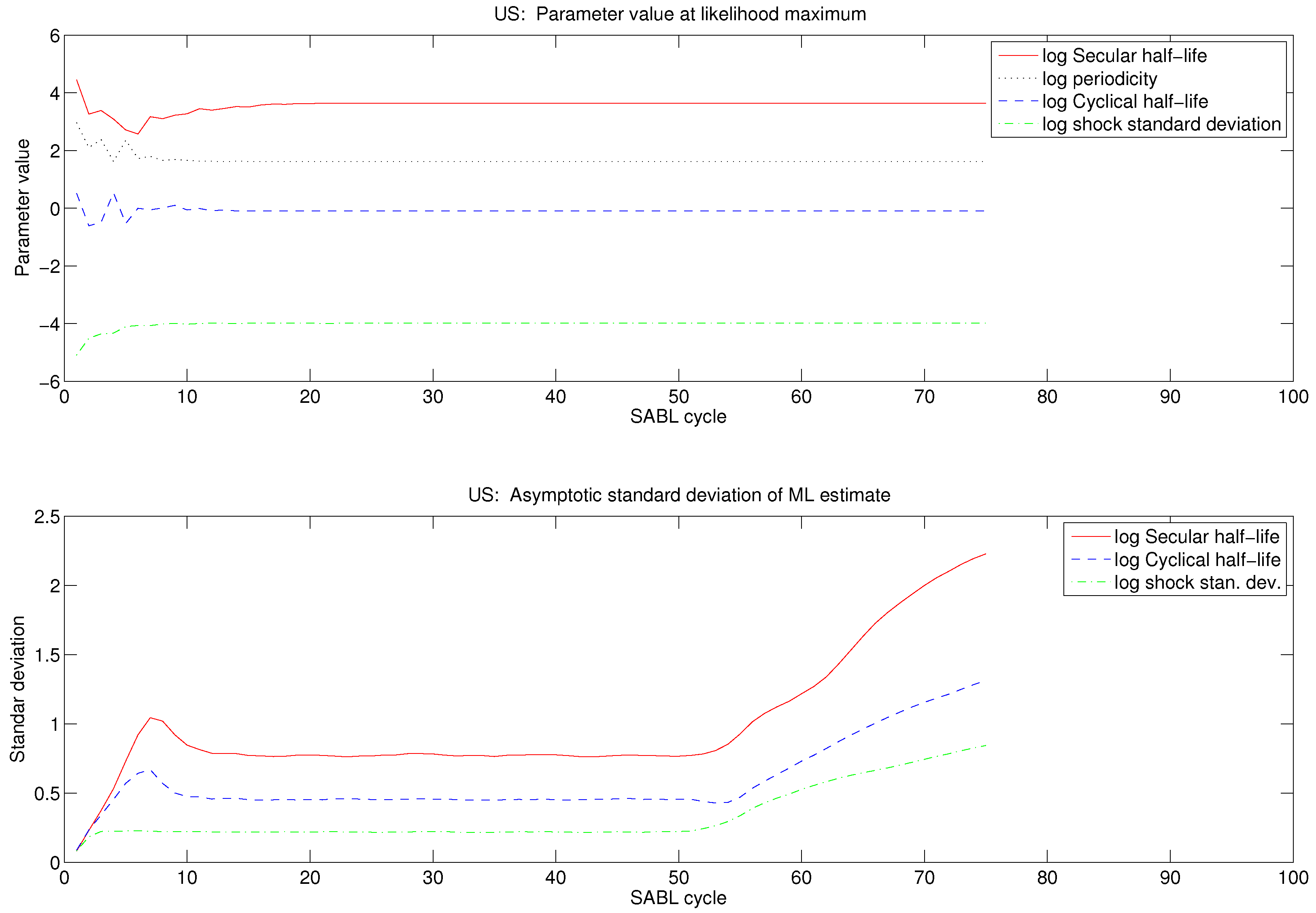
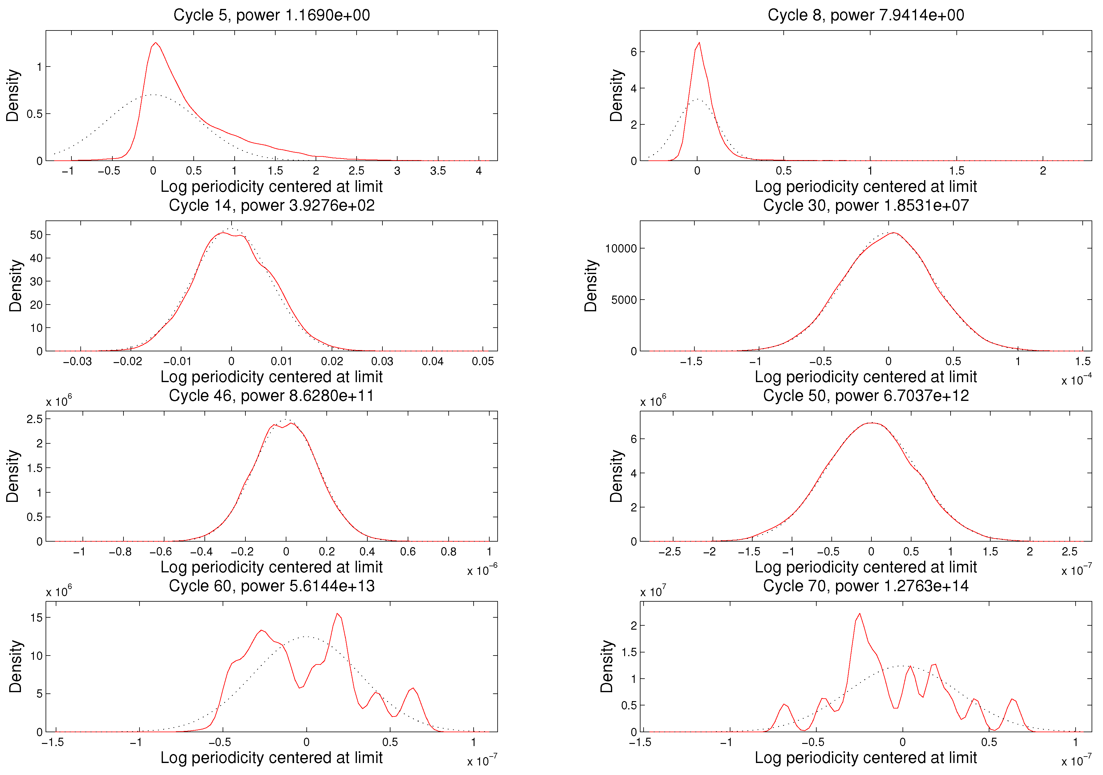
Important practical questions are SABL termination criteria and the cycle(s) ℓ whose particles are used to approximate $V=H^{-1}$ using $V_{\ell }$. Clearly the cycles chosen to approximate v must be cycles after the asymptotic power increase ratio has been closely attained, evidenced by fluctuations above and below ρ over a sequence of successive cycles. One may also wish to apply criteria for concentration of the distribution of the particles ${\theta }_{jn}$ or the distribution of the objective $log\left[k\left({\theta }_{jn}\right)\right]$. There seems no reason to continue beyond these points.

In fact, if cycles are allowed to continue, then eventually the algorithm encounters the limits of 64-bit arithmetic in distinguishing between values of $logk\left({\theta }_{jn}\right)$. The telltale evidence of this condition is that the evaluation of $logk\left({\theta }_{jn}\right)$ at different particles ${\theta }_{jn}$ reflects the bits of the mantissa corresponding to lowest significance. Experience with examples like the one in this paper strongly suggests that the sequence of power increase ratios $\left\{{\rho }_{\ell }\right\}$ exhibits three episodes, going to the limits of 64-bit arithmetic.

• In the early cycles ${\rho }_{\ell }$ differs substantially from ρ. The most common pattern observed is that in the early cycles ${\rho }_{\ell }$ exceeds ρ, drifting downward toward ρ.
• In the middle cycles ${\rho }_{\ell }$fluctuates around ρ, fluctuations being smaller the larger the number of particles. With the default number of particles in the SABL software ($2^{14}$) fluctuations are less than 10% and commonly less than 5%. In these cycles the particles ${\theta }^{\left(\ell \right)}$ have a distribution that is hard to distinguish from multivariate normal.
• In the later cycles ${\rho }_{\ell }$ drops well below ρ and fluctuates erratically. The reason is that variation in the particles is no longer dominated by the asymptotics outlined above: the limits of machine precision become increasingly important. (In the limit the distribution can become bizarre, as detailed in [2]). The random walk Gaussian Metropolis steps in the M phase are poorly suited to the the objective function now dominated by lower-order bit arithmetic, relative numerical efficiency is poor, and the particle distribution provides a poor source distribution in the C phase, leading to smaller increases in power in each cycle.

These patterns are generally evident in a plot of $log{\rho }_{\ell }$ as a function of cycles ℓ, in which the middle cycles exhibit as a nearly flat portion of an otherwise generally decreasing function of ℓ. Any one of the middle cycles is a natural point to harvest the asymptotic variance matrix of the maximum likelihood estimator, as described above. At this point it is also natural to take as the MLE $\widehat{\theta }=$ $arg{max}_{\ell ,j,n}logk\left({\theta }_{jn}^{\left(\ell \right)}\right)$. Experience suggests that the accuracy of the MLE, so computed, is well beyond the number of digits typically reported.

5.3. Relationship to the Simulated Annealing Literature

The technique of simulated annealing was introduced over 30 years ago [10] and is now widely applied in science and engineering. Applications in statistics and econometrics are very rare and most econometricians do not include it in their suite of approaches to maximization problems. This is so despite the fact that [11] demonstrated the method’s utility in that capacity in a Journal of Econometrics paper that ranks 18th (out of thousands) by citation in the simulated annealing literature, and ninth in the citation rankings of articles in that journal. Almost all of the citations come from the science and engineering literature, very few from economics or statistics.

The simulated annealing literature also uses a sequence of increasing powers of the objective function, but casts the sequence as its inverse $r_{\ell }^{-1}$, known as temperature. Thus temperature decreases as the algorithm proceeds and this is responsible for its name. In the original version, and indeed most applications since, it may be regarded as a simple version of the SABL algorithm in which there is one particle and no S phase. Since there is no distribution of particles, neither the sequence of increasing powers in the C phase nor the variance in the Metropolis steps of the M phase can be constructed algorithmically as they are in SABL. Instead they must be provided directly by the user in each application.

Choosing a sequence of increasing powers (decreasing temperatures) that results in reasonable efficiency—or even works at all—has been a challenge. Typical applications, even by experienced practitioners, involve trial, error and tinkering with temperature reduction schedules. The choice of the variance matrix for the Metropolis step similarly must be tailored to each application, a procedure familiar to many Bayesian econometricians and statisticians who have used the Metropolis random walk for Bayesian inference. In simulated annealing, this variance matrix must be related systematically to temperature (power).

Very recently the simulated annealing literature has begun to adopt parallel chains of arguments–particles, in the terminology of this paper. Zhou and Chen [12] is representative. I am not aware of any work in this literature that attempts to use the parallel chains to address the temperature reduction problem and the Metropolis variance matrix problem systematically. Thus the method still suffers from this very substantial overhead in application. Once acceptable solutions to these problems have been found by trial and error, none begins to approach the standard of computing the maximizing argument to the limits of machine precision attained by SABL. Geweke and Frischknecht [2] draws an explicit comparison using the test problems in [12], showing that SABL achieves machine precision with about the same number of floating point operations used in the methods of that paper, which in fact do not even determine the optimizing values to even three significant figures in all cases.

6. Maximum Likelihood Estimation of Half-Lives and Periods

This section illustrates optimization in SABL for the case of maximum likelihood using the U.S. data. As with the posterior distribution results are quite similar across countries.

6.1. Performance of the Optimization Algorithm

Figure 4 provides a global perspective on the behavior of the algorithm. The northwest panel provides the power r (of the likelihood function in each cycle of the SABL algorithm), and the south east panel displays the power increase ratio. In the terminology of the simulated annealing literature the temperature is the inverse of power, and the analogue of temperature for the northwest panel would simply flip the graph about a horizontal axis of rotation at ${10}^0$. The temperature decay and power increase ratios are identical. In both cases it is straightforward to identify the cycles over which the geometric rate of increase is constant, roughly cycles 14 through 46. The power increase (temperature decay) ratio fluctuates about the theoretical value ρ stated in (21) and shown by the dotted line in the southeast panel. The last cycle in which the ratio exceeds ρ is $\ell =44$. Computation to this point required 44 seconds using the same hardware and software used for the posterior distribution in Section 4. The difference is due to the fact that Bayesian inference required only 5 cycles (Table 1).

The cycles of constant power increase ratio end when the limitations of floating point arithmetic begin to disguise the true quadratic nature of the log-likelihood function in the neighborhood of the maximum. Up to this point the Metropolis random walk is effective in mixing particles in the M phase, which may be seen in the fact that at most 8 iteration are required to attain the RNE criterion of 0.4 that ends the M phase and the cycle, whereas from iteration 49 onward the convergence criterion is never met and the M phase goes to the default limit of 100 iterations. After iteration 48 (roughly) RNE drops rapidly, the weight function in the C phase is poor, and the number of distinct particles (southwest panel) deteriorates quickly. By iteration 60 there are only about 100 distinct particles.

The northeast panel provides a complimentary perspective on the limitations imposed by machine arithmetic. So long as the power increase ratio is near ρ, the standard deviation of the log-likelihood objective function is very nearly inversely proportional to power. In all events differences between real numbers are multiples of what is known as “machine epsilon”, which for conventional 64-bit floating point representation is $\epsilon =2.22\times {10}^{-16}$. This graininess becomes a factor beyond about iteration 48. Standard deviation of the objective function, across particles, decreases toward ε, shown by the dotted line in the northeast panel. Eventually the objective function behaves like a step function and except for extremely simply objective functions the steps appear random to the eye.

Figure 5 provides perspectives on the maximum likelihood estimates and asymptotic standard errors in each cycle of the SABL algorithm. The maximum likelihood estimates in the upper panel are constant (to the accuracy of the plot) beyond about cycle 20. The complications of machine arithmetic affect only the evaluated shape of the surface, not its location, and so these estimates remain unaffected. The deduction of asymptotic standard errors from the distribution of the particles, on the other hand, is closely tied to multivariate normal distribution of particles. It is constant over the same range that the power increase ratio is constant, and exhibits about the same amplitude of relative fluctuations. Beyond about cycle 54 it increases, due to the fact that the limitations of 64-bit arithmetic introduce variation in particles that is significant relative to the actual value, meaning that it continues to increase. The lower panel of Figure 5 supports the convergence criterion of last cycle $\left(\ell =46\right)$ in which the power decay ratio exceeds ρ.

Figure 6 supplements these perspectives by providing the distribution of the parameter ${\theta }_4=log\left(p\right)$ in some cycles of interest. (Result for other parameters are qualitatively similar.) The solid line provides the kernel smoothed estimate of the distribution of particles, the dotted line the Gaussian distribution corresponding to particle mean and variance. In all cases the deviation of values from the final maximum likelihood estimate are shown to make the horizontal axis ticks readily interpretable. Prior to the cycles of constant power increase ratio the shape of the distribution moves from the posterior distribution portrayed in Figure 1 (cycle 5 is very close) to the quadratic expansion of the log-likelihood about the maximum likelihood estimate, scaled by power. Beyond that point the distribution becomes erratic as it is increasingly corrupted by the limitations of machine arithmetic. The Metropolis step, with its Gaussian proposal is increasingly ineffective; to appreciate this fully, recall that the Metropolis step is dealing with this behavior in five dimensions at once.

These results support the idea that iteration to maximum likelihood can halt when the power increase ratio begins to fall from the neighborhood of the value ρ implied by a quadratic objective function of the relevant dimension. At the last cycle in which this ratio exceeds ρ , the maximum likelihood estimate can be taken to be the particle providing the highest log-likelihood and the asymptotic variance can be taken to be particle variance multiplied by power $r_{\ell }$.

6.2. Findings

It is straightforward to compute maximum likelihood estimates and their asymptotic variance as just described. We compare these results with two other approaches. One is the posterior distribution presented in Section 4. The other begins with the closed-form maximum likelihood (least squares) estimate of $\left(\beta ,\sigma \right)$ in (1) and transforms the estimate to $\left({\beta }_0,log\left(h_s\right),log\left(h_c\right),log\left(p\right),log\left(\sigma \right)\right)$ as described in that section. By the invariance property of maximum likelihood estimates, these should be the same as those obtained using the methods of Section 5. From the last procedure we also compute the distribution of $\left({\beta }_0,log\left(h_s\right),log\left(h_c\right),log\left(p\right),log\left(\sigma \right)\right)$ obtained by mapping from the asymptotic distribution of the maximum likelihood estimator of $\left(\beta ,{\sigma }^2\right)$. This will not be the same as asymptotic distribution the direct maximum likelihood estimates. But it comes very close to the posterior distribution in [7] because the prior distribution in that work was $p\left(\beta .\sigma \right)\propto {\sigma }^{-1}$ subject to the constraints of stationarity and two complex roots of the lag operator generating polynomial. (Those constraints are satisfied in over 99% of the draws from the asymptotic normal distribution of $\left(\beta ,\sigma \right)$ here.) Thus, this comparison enables us to examining the influence of two quite different prior distributions for $\left({\beta }_0,log\left(h_s\right),log\left(h_c\right),log\left(p\right),log\left(\sigma \right)\right)$.

Table 5. US posterior moments and maximum likelihood estimates.

	Posterior		Direct ML, θ		OLS Indirect ML
Parameter	mean	st. dev.	MLE	st. dev.	MLE	st. dev.
Secular $log\left(h_s\right)$	4.056	0.667	3.646	0.767	3.646	0.866
Cyclical $log\left(h_c\right)$	−0.584	0.548	−0.096	0.457	−0.096	0.406
Period $log\left(p\right)$	2.045	0.565	1.621	0.148	1.621	0.231
Shock $log\left(\sigma \right)$	−3.917	0.112	−3.984	0.109	−3.984	0.117

provides the first two moments of each parameter for the three cases. Those for the posterior distribution are the same as in Table 2. The maximum likelihood estimates of $log\left(h_c\right)$ and $log\left(p\right)$ differ from the posterior means, by more than one standard error in the first case and by over two maximum likelihood standard errors in the second (using the metric of the direct ML standard error in each case). Except for $log\left(p\right)$ the posterior standard deviation and the ML asymptotic standard errors are similar. For $log\left(p\right)$ the direct ML asymptotic standard error is smaller than the posterior standard deviation by a factor of almost 4 and the indirect ML asymptotic standard error by a factor of over 2. This gross divergence for $log\left(p\right)$ is consistent with the posterior density in the southwest panel of Figure 1, whose model is much more sharply defined than is the mode of a normal distribution. The conventional local expansion of the log-likelihood function is unrepresentative of its global behavior in the case of $log\left(p\right)$.

Figure 7 provides another perspective on the comparison between the three approaches to inference, for the joint distribution of secular and cyclical half-life (left panels) and the joint distribution of period and cyclical half-life (right panels). To facilitate comparison the axes are identical in each column and were selected so as to exclude the 0.25% smallest and 0.25% largest points out of 820 selected from the 16,348 particles in the posterior distribution. The number of points plotted in the last two rows is almost 820 since the dispersions there are smaller. The horizontal and vertical lines are the same in each column, intersecting at the maximum likelihood estimate, which is indicated by the circle in the last two rows. In the top pair of panels the circle is the mean of the posterior distribution and the cross is the median. The smaller dispersion of the parameters under the asymptotic ML distributions, especially for $log\left(p\right)$, is striking in these figures. So, too, are the differences in shape. The joint distribution under the direct ML asymptotic expansion is Gaussian by construction; as already documented and well-understood, the posterior distribution is not; but the indirect ML distribution is also non-Gaussian because the transformation from $\left(\beta ,\sigma \right)$ to θ is nonlinear.

The indirect ML asymptotic expansion is very close to the exact posterior distribution using the conventional improper prior distribution $p\left(\beta .\sigma \right)\propto {\sigma }^{-1}$, sometimes called the Jeffreys prior on (less precisely) “diffuse” or “uninformative.”uninformative prior. This is in fact not a Jeffreys prior for linear regression except when it reduces to mean estimation. Whereas the prior in β is flat, the implied prior for θ is not due to the Jacobian implied by the nonlinear transformation in equations (2) through (4). The fact that “diffuse ”or “uninformative”prior distribution can be vague, slippery or vacuous concepts is sometimes missed by Bayesian econometricians, like [7].

7. Conclusions

The utility of econometric models hinges in no small part on their direct connection to the concepts economists use to create these models and interpret the results of inference. In the example presented in this paper it was possible to replace almost all of the conventional parameters that are convenient for statistical models with such concepts. In many other cases this can be done to partial but significant degree: dynamic stochastic general equilibrium models as utilized in central banks constitute an important class of such examples in macroeconomics. Similar examples in microeconomics and the business sector are also common. If the econometrician is to interpret and communicate findings to the decision-making client, this is important. For the Bayesian econometrician attempting to elicit and incorporate client prior distributions it is even more compelling.

As a practical matter it is equally important for econometricians to be able to bring models to data quickly, avoiding the need for case-by-case special treatments in deriving auxiliary analytical results and tuning computational algorithms. These steps require significant additional time and specialized skills that can place econometric approaches at an overwhelming disadvantage in competition with alternatives (like machine learning) that on their own may not serve the client as well.

The SABL algorithm illustrated in this paper is a tool that addresses these objectives. For a new application, and even for a new model, it presents much lower barriers to entry than do most existing procedures in Bayesian and non-Bayesian econometrics. This is a strong claim, and this paper is a small illustration in support of that claim. Further such illustrations are forthcoming.