Use of the Principles of Maximum Entropy and Maximum Relative Entropy for the Determination of Uncertain Parameter Distributions in Engineering Applications

Abstract

The determination of the probability distribution function (PDF) of uncertain input and model parameters in engineering application codes is an issue of importance for uncertainty quantification methods. One of the approaches that can be used for the PDF determination of input and model parameters is the application of methods based on the maximum entropy principle (MEP) and the maximum relative entropy (MREP). These methods determine the PDF that maximizes the information entropy when only partial information about the parameter distribution is known, such as some moments of the distribution and its support. In addition, this paper shows the application of the MREP to update the PDF when the parameter must fulfill some technical specifications (TS) imposed by the regulations. Three computer programs have been developed: GEDIPA, which provides the parameter PDF using empirical distribution function (EDF) methods; UNTHERCO, which performs the Monte Carlo sampling on the parameter distribution; and DCP, which updates the PDF considering the TS and the MREP. Finally, the paper displays several applications and examples for the determination of the PDF applying the MEP and the MREP, and the influence of several factors on the PDF.

1. Introduction

In many industrial applications, researchers, engineers, and organizations use computer codes that contain the state of the art of a given branch of engineering. These codes use, in general, physical models that are the state of the art for a given application, for instance CFD (computational fluid dynamics) codes such as ANSYS-CFX or STAR-CD for fluid engineering applications, FEM (Finite Element Method) codes as ANSYS for mechanical engineering applications, thermal-hydraulics codes as RELAP or TRACE for nuclear engineering applications, and so on [1,2,3]. In general, these codes need a set of input data that can be classified as: initial and boundary conditions, geometric data, physical property data, and model parameter data. The methodologies known as BEPU, meaning Best-Estimate Plus Uncertainty, try to estimate the uncertainty in the code response once the uncertainty in the input and model data have been obtained and propagated from the input to the output [4,5]. These methodologies provide a set of output results plus their uncertainties in the form of tolerance regions with prescribed levels of coverage and confidence, usually 95/95, meaning a 95% of coverage and 95% confidence. Depending on the type of computational code, the number of uncertain input parameters can be small or large; if the number of uncertain parameters is large, there exist some techniques, as the sensitivity analysis or the PIRT (phenomena identification and ranking table), which allow the reduction of the number of uncertain parameters to only those that have a certain degree of influence on the output results, or, in the case of nuclear engineering, on the critical safety output parameters [5,6].

One of the main problems found in this type of work is the determination of the probability distribution of the input and model parameters. Occasionally, we only know the parametric family of the distribution of a given uncertain parameter X, but the distribution parameters $\mathit{\theta }({\theta }_1,{\theta }_2,\dots ,{\theta }_n)$ are unknown. So, the set of unknown parameters of the probability distribution function (PDF) $p_X(x|\mathit{\theta })$ must be determined. Other times, we do not know the distribution of the parameter, but we know some moments of the distributions, so we need a method to obtain the parameter distribution from the partial information that we have on the moments. In addition, it is possible that regulatory restrictions are imposed on some input parameters. For instance, the nuclear regulatory agencies around the world impose the so called ‘technical specifications’ (TS) that must be fulfilled by some operational plant parameters, and surveillances are periodically performed to know if the plant parameters verify these TS [7,8]. These additional restrictions can modify the PDF of a given parameter, so we need methods to determine the parameter distributions from the available information and, at the same time, to determine the change in these distributions produced by the TS. Notice that to know if the TS are verified, the parameter values of some components are surveilled periodically and if its values are not within the intervals indicated by the TS, then, modifications are performed to change its values to fulfill the TS. The application of the MEP and the MREP provides a method to determine the PDF of the unknown parameters when partial information is known. The methodology consists of selecting the PDF that maximizes the Shannon information entropy and, at the same time, fulfills the restrictions imposed by the known information in the form of known moments, these ideas were initiated by Shannon and Jaynes [9,10,11,12] and then were further elaborated by Mead and Papanicolau [13], Montroll and Shlesinger [14], Shore and Johnson [15], among other researchers.

The application of the MEP to engineering problems has been performed in the past by different authors to know the parameter distribution for some cases [5,16,17,18,19,20], when limited information was known about the parameter distribution, for instance, some moments of the distribution and its support interval. This case is studied in this paper and two additional ones that need the application of the MREP: the first case is when new information is available on a given parameter and we need to update the distribution considering the previous one and the new available information, this problem can also be studied by Bayesian methods as in Caticha and Preuss [21]. The second case is when there are some technical specification (TS) that can have some influence on parameter distribution. These technical specifications can fix some acceptance intervals for some parameters and, also, they establish detailed instructions to perform periodical surveillance to check the fulfillment of the TS [7,22].

The main objective of the paper is to develop a methodology to obtain the unknown probability distribution functions of the parameters that enter into BEPU analysis when only partial information is available about these parameters using the MEP, this information could be provided as some known distribution moments or support. A second objective is the updating of the parameter distribution when new information is provided. In this case, the MREP is used to update the PDF, using the old PDF as ranking function. The third objective is how to consider the effect of the technical specifications imposed by regulatory authorities on the probability distributions of the input parameters that must fulfill these TS. Finally, a four objective is to develop tools to apply these developments to real cases found in the applications. These developments are of relevance for present and future applications of BEPU and uncertainty quantification of the results of many engineering applications.

The aim of the paper is to assemble, in a single paper, the basic ideas of the maximum entropy and the maximum relative entropy principles, and the applications of these principles to solve common problems found in BEPU engineering analysis, including the technical specifications imposed by the regulations. In addition, a few key deductions have been explained with detail in order that people learns how to apply these techniques to solve specific problems.

The paper has been organized as follows:

Section 2 gives a brief introduction on uncertainty quantification in engineering codes. The goal of this section is to analyze the fields where the principles of maximum entropy and maximum relative entropy can be applied.

In Section 3.1, we explain how to apply the principle of maximum entropy to the determination of the probability distribution function when some moments of the distribution are known; whereas in Section 3.2, we explain the application of the maximum relative entropy to update PDF when new information is available; finally, in Section 3.3 it is explained the application of the MREP to the determination of the PDF considering the technical specifications imposed by regulatory authorities.

In Section 4, we give some examples of the application of the MEP and the MREP to some cases that can appear in the applications. Section 4.1 shows the application of the MEP and the MREP to the case of known support $\left[-\infty ,\infty \right]$ and previously known mean $\mathsf{\mu }$, and variance ${\mathsf{\sigma }}^2$ when the TS impose an acceptance interval $\left[\mathrm{L},\mathrm{U}\right]$ with coverage $\mathsf{\gamma }$ and confidence $\mathsf{\beta }$. In Section 4.2, we explain the application of the MREP to several cases with previously known distributions when new information is known with and without technical specifications (TS). 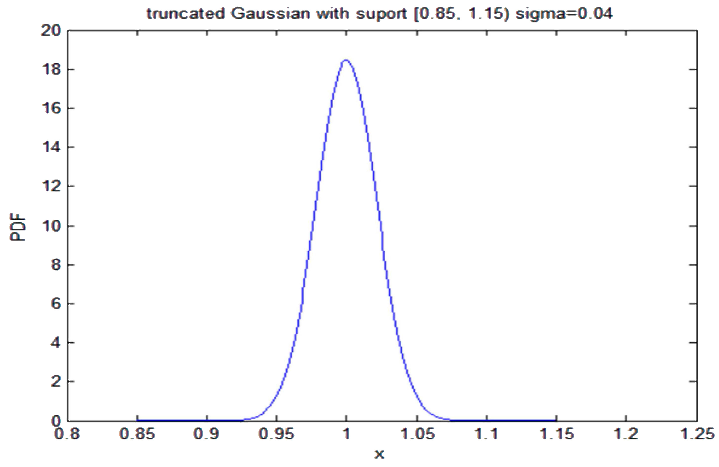In Section 4.3, we explain the application of the MREP to the case of a parameter with a previous truncated Gaussian distribution, for which the updated data have the same mean and support but different variance. Finally, Section 4.4 of this paper shows the results obtained applying the MEP to several cases found in the applications.

In Section 5, we explain the programs that have been built to apply the previous development to some real cases, also in this section we display some applications of the previous programs to some particular cases.

Finally, in Section 6 we discuss the main findings and conclusions of the paper.

2. Uncertainty Quantification in Thermal-Hydraulics and CFD Codes

In this section, we give some brief outlines about the possible fields were the application of the maximum entropy principle and the maximum relative entropy principle could be useful.

2.1. BEPU Methodologies in Nuclear Engineering Applications

Deterministic safety analysis (DSA) is the analytic tool used in the design of nuclear power plants. DSA methodologies are used to calculate a number of safety magnitudes as defined by regulatory authorities for different ‘design basis accidents’. DSA methodologies can be roughly classified in two categories conservative and realistic (BEPU). Computational codes are used in DSA methodologies to obtain the safety magnitudes of interest. Conservative methodologies use predictive models and assumptions that introduce a pessimistic bias on calculated safety magnitudes. For this reason, they do not need an uncertainty analysis of the results.

The acceptance criteria in these conservative methodologies are simple, considering that the predictive model of the computational code can be viewed as a multidimensional function

$$\mathit{Y}=\mathit{R}\left(\mathit{X}\right) \mathrm{with} \mathit{X}\in {ℝ}^n, \mathit{Y}\in {ℝ}^m$$

(1)

where $\mathit{Y}$ represents the output response of the code (i.e., the calculated safety magnitudes for a given design basis transient or accident), that is generally multidimensional, and consists in a set of values of the safety parameters of interest versus time. The code can be considered as a certain function transforming the input and model data $\mathit{X}$ in the code output $\mathit{Y}$for a given scenario, that describes a certain transient or accident type. In these kinds of methodologies, where very conservative models and input parameter data are used, the acceptance criteria are very simple and express the fact that the output safety variables $\mathit{Y}$ computed by the code must be located inside a prescribed region of the code output space, called the ’safety region’ (SR). The safety region specifies certain limits for the components of $\mathit{Y}$ to assure the safety of the design for the considered scenario. If the output vector remains inside this region, the safety is guaranteed for the considered scenario so we must have

$$\mathit{Y}\in SR\subset {ℝ}^m$$

(2)

The components of the vector $\mathit{Y}$ are plant magnitudes like temperatures, pressures, and degrees of oxidation at specific reactor locations.

The other kind of methodologies, known as realistic or BEPU (Best-Estimate Plus Uncertainty) methodologies, use models and input data values that contains the state of the art for the physical models and numerical methods used to solve a set of problems. Because the parameter models and input data contains a certain degree of uncertainty, and this uncertainty is propagated from the input to the output through the code. Then, in the BEPU methodologies, the acceptance criteria with a degree of coverage ${\gamma }_0$ and confidence ${\beta }_0$ is written, in a probabilistic way, as follows [4]

$$Pro{b}_S\left(Pro{b}_{\mathit{Y}}\left(\mathit{Y}\in SR\right) \ge {\gamma }_0\right) \ge {\beta }_0$$

(3)

Equation (3) states that $\mathit{Y}$ must be inside $SR$ with a probability of at least γ₀ (termed level of coverage) and a statistical confidence β₀ (termed level of confidence). The pair γ₀/β₀ is termed level of tolerance of the criterion (3).

One immediately observes that the acceptance criteria in the BEPU methodologies adopt a more complex form than in the conservative methodologies. Equation (3) contains two nested probabilities, the inner one refers to the uncertainty on $\mathit{Y},$ propagated from the uncertain input $\mathit{X}$ and model data to the output for a sample of finite size N. This uncertainty is produced by the random nature of $\mathit{X},$ that generally are sampled by Monte Carlo and then propagated by the code to the output. The outer probability is due to the finite size of the sample S used to perform the Monte Carlo sampling and propagate the results from the input to the output, if we choose another samples of the same size the results will be different but at least ${\beta }_0 \times 100\%$ of the results will have a degree of coverage bigger than ${\gamma }_0.$

To perform the BEPU methodologies, one key point is to use Monte Carlo to perform the random sampling over the distribution of the uncertain input data and model parameters. However, to perform this sampling one needs the PDF of the parameter to be sampled. Here the principles of maximum entropy and maximum relative entropy enter in action. Because the parameter distribution is not always known for all the parameters and we have in some cases only a partial knowledge about some moments of the parameters and the support of the distribution, these two principles MEP and MREP can be used to obtain the PDF that maximizes the entropy in the first case and the relative entropy in the second case and, at the same time, satisfy the restrictions imposed by the partial information known about the parameters. Another important issue that appears in nuclear engineering, and in some branch of engineering subject to technical specifications (TS) on certain operational parameters, is the influence of these specifications on the PDF. This issue is also studied in the next section.

2.2. Application of the MEP and the MREP to the Determination of the Uncertainty in the Results of Heat Transfer Codes and CFD Codes

Another field of application of the MEP and the MREP is to the determination of the PDF of the input parameters of heat transfer and CFD problems. If we have partial information on some parameter that fixes the boundary conditions of a given heat transfer problem, the use of the MEP or the MREP allow us to obtain the parameter PDF that maximizes the information entropy and, at the same time, satisfy the restrictions imposed by the partial knowledge on the parameter. For instance, the VV20 ASME standard [23] set the following problem: let us assume that one wants to obtain the temperature distribution versus time for a planar 1D slab exposed to a constant heat flux $q^{″}$ at one face and adiabatic condition on the other face, and with a uniform initial temperature distribution at time t = 0, ${\left\{T_{i,0}=constant\right\}}_{i=1}^n$, being n the number of nodes. The uncertainty in the computed temperatures $T_i$ (output) at different times and different nodes for this simple case is due to the uncertainty in the heat flux $q^{″}$, the uncertainty in the conductivity k of the slab material, the uncertainty in the product $\rho c_p$ (density times the specific heat at constant pressure), and the uncertainty in the initial temperatures. So, the vector of input data that are uncertain for this simple case is $\left\{q^{″}, k,\rho c_p ,T_{i,0}\right\}$. One of the most common techniques used to evaluate the distribution of the output is using the Monte Carlo method that requires N random samples to be obtained by sampling on the PDF of each parameter, and then to run the code N times and to obtain N samples of the output. The inconvenience of this method is that the convergence is bad. So, an alternative to this method, is the latin hypercube sampling (LHS) that requires the knowledge of the cumulative distribution function of the input parameters. In this method, the range of each uncertain parameter is divided into $n_{LHS}$ bands of equal probability. Within each band a sample is drawn from the parameter PDF. The result is a matrix of $n_{LHS}\times n_p$ values, being $n_p$ the number of uncertain parameters. To assure full coverage, the input and model parameters are combined in a random way as described by Helton and Davies [24,25]: “The $n_{LHS}$ values obtained for $X_1$ are paired at random and without replacement with the $n_{LHS}$ obtained for $X_2$. These $n_{LHS}$ pairs are combined in a in random manner and without replacement with the $n_{LHS}$ of $X_3$, to obtain $n_{LHS}$ triples, and so on...”. Then we proceed by running the code $n_{LHS}$ times with the $n_p$ tuples being different from one run to the other. Finally, the mean and the variance are estimated by standard statistical methods.

3. Application of the Maximum Entropy Principle and the Maximum Relative Entropy Principle to the Determination of the PDF with and without Technical Specifications

3.1. Application of the MEP to the Case of Knowledge of Some Moments of the Distribution and Its Support

When the probability distribution function of a given parameter X with continuous distribution is unknown and some moments of the parameter distribution are known, then, we apply the maximum entropy principle (MEP) to obtain the parameter distribution following the ideas of Jaynes [11,12]. If $f_X\left(x\right)$ denotes the probability density function of the random parameter X, and $F_X\left(x\right)$ the cumulative distribution function, Claude Shannon defined the concept of information entropy H as a measurement of the uncertainty associated to the result of a given process [9]. If X has a compact support, i.e., the random variable X can take values between a and b, with b > a, being [a, b] the distribution support; then the Shannon information entropy is defined by the expression [5,9,10,16]

$$H=-\underset{a}{\overset{b}{\int }}{f}_X\left(x\right)\log \left(f_X\left(x\right)\right)dx=-\underset{a}{\overset{b}{\int }}\log \left(f_X\left(x\right)\right)d{F}_X$$

(4)

Usually, we have statistical information about some moments of the PDF, defined in the general form

$$\underset{a}{\overset{b}{\int }}{g}_i\left(x\right)f_X\left(x\right)dx=\mu \left(g_i\right)={\mu }_i, i=0,1, 2,\dots ,n$$

(5)

In general, the functions $g_i\left(x\right)$ define the different moments of the distribution function of the parameter $X$, where the index $i$ runs from 1 to the number n of previously known moments, the index 0 is reserved for the normalization condition of the PDF, i.e., when we make $g_0\left(x\right)=1$, and ${\mu }_0=1.$

The problem to be solved in information theory when applying the MEP is to obtain the PDF expression $f_X\left(x\right)$ that maximizes the information entropy and, at the same time, obeys the set of restrictions displayed in Equation (5). To solve this problem, variational calculus is generally used and, first, we build the following functional $J\left[f_X\left(x\right)\right]$ that includes the restrictions of Equation (5) by means of the Lagrange multiplier method

$$J\left[f_X\right]=-\underset{a}{\overset{b}{\int }}{f}_X\left(x\right)\log (f_X\left(x\right)) dx+{\displaystyle \sum }_{i=0}^n{\lambda }_i\left[\underset{a}{\overset{b}{\int }}dx{g}_i\left(x\right)f_X\left(x\right) - {\mu }_i\right]$$

(6)

The variational calculus looks for the PDF $f_X\left(x\right)$ that maximizes the information entropy and is consistent with the available constraining information. So that one looks for the PDF $f_X\left(x\right)$ and the Lagrange multipliers ${\lambda }_i$ values such that we have an extreme of the functional $J\left[f_X\left(x\right)\right]$, and at the same time the set of restrictions (5) are satisfied. To find this extreme, one considers an arbitrary perturbation $\alpha \delta f_X\left(x\right)$ that vanishes at the end points a and b of the support interval. According to the variational calculus, the first variation $\delta J\left[f_X\left(x\right)\right]$ of the functional $J\left[f_X\left(x\right)\right]$ is given by

$$\delta J={\left[\frac{\partial J\left(f_X\left(x\right)+\alpha \delta f_X\left(x\right)\right)}{\partial \alpha }\right]}_{\alpha =0}=0$$

(7)

Performing the calculations in Equation (7) because of Equation (6) yields

$$\delta J=\underset{a}{\overset{b}{\int }}\delta f_X\left(x\right)\left(-\log \left(f_X\left(x\right)\right)-1+{\displaystyle \sum }_{i=0}^N{\lambda }_i{g}_i\left(x\right)\right)dx=0$$

(8)

Due to the arbitrary character of the perturbation $\delta f_X\left(x\right)$ the term inside the brackets in Equation (8) must be zero so it is obtained for the PDF of the parameter the following expression

$$f_X\left(x\right)=\exp \left\{-1+{\displaystyle \sum }_{i=0}^N{\lambda }_i{g}_i\left(x\right)\right\}$$

(9)

The values of the constants ${\lambda }_i$ are obtained from the available information on the distribution moments given by the set of Equation (5). In general, to obtain the parameter values of ${\lambda }_i$ it is necessary to solve a non-linear system of algebraic equations as will be shown later.

3.2. Application of the Maximum Relative Entropy (MREP) to the Case of New Updating Information

The principle of maximum relative entropy (MREP) can be applied in the following two cases. The first one is to update a previous or ‘a priori’ PDF denoted by $f_X\left(x\right)$ of a given parameter when new information is available, this information can be provided as new data or moments of the distribution. The second case is when a regulatory body impose some specifications or restrictions on the parameter values that modify the parameter distribution, this second case will be studied separately.

Let us now study the first case, assuming that the parameter follows an unknown probability density $q_X\left(x\right)$ in the support interval $\left[a, b\right]$. Let us assume that we have a previous estimation or ‘a priori’ estimation $f_X\left(x\right)$ of the true PDF. Then, at a later time or ‘a posteriori’, we have obtained additional information as moments or data of the unknown PDF. Therefore, we need to update the probability distribution considering both the previously known distribution and the new information or data available on the parameter. This goal can be achieved using the principle of the maximum relative entropy (MREP). Caticha and Preuss [21] used this principle to develop updating methods that are systematic and objective, they arrive to the conclusion that the unknown probability distribution $q_X\left(x\right)$ should be ranked according to its relative entropy with respect to the previously known PDF $f_X\left(x\right)$, this means

$$S\left(q_X,f_X\right)=-\underset{a}{\overset{b}{\int }}dx q_X\left(x\right)\log \left(\frac{q_X\left(x\right)}{f_X\left(x\right)}\right)$$

(10)

The new information generally comes as a set of known moments ${\mu }_i^{\prime }$ of the unknown distribution $q_X\left(x\right)$ given by

$$E\left(g_i\right)={\int }_a^{b}dx g_i\left(x\right)q_X\left(x\right)={\mu }_i^{\prime }, i=0,1,2,\dots n^{\prime }$$

(11)

where the new moment values could be the same or different values from the previous ones, so we distinguish the new values with a prime, also the number of new moments $n^{\prime }$ could be different. To maximize the relative entropy subject to the new restrictions we build the new functional $F\left(q_X,f_X\right)$ with Lagrange multipliers ${\lambda }_i^{\prime }$ and moments ${\mu }_i^{\prime }$ as

$$F\left(q_X,f_X\right)=-\underset{a}{\overset{b}{\int }}dxq\left(x\right)\log \left(\frac{q_X\left(x\right)}{f_X\left(x\right)}\right) + {\displaystyle \sum }_{i=0}^{n^{\prime }}{\lambda }_i^{\prime }\left[{\int }_a^{b}dx g_i\left(x\right)q\left(x\right)-{\mu }_i^{\prime }\right]$$

(12)

Then, we use variational calculus again to obtain the PDF that maximizes the relative entropy and, at the same time, satisfies the updated moment values, i.e., we set the first variation of the functional $F\left(q_X,f_X\right)$ to zero

$$\delta F\left(q_X,f_X\right)={\left[\frac{\partial F\left(q_X\left(x\right) + \alpha \delta q_X\left(x\right), f_X\left(x\right)\right)}{\partial \alpha }\right]}_{\alpha =0}=0$$

(13)

This calculation yields, because the arbitrary character of the perturbation $\delta q_X\left(x\right)$, the result

$$q_X\left(x\right)=f_X\left(x\right)\exp \left\{-1+{\displaystyle \sum }_{i=0}^n{\lambda }_i^{\prime }{g}_i\left(x\right)\right\}=f_X\left(x\right)C\left(x\right)$$

(14)

The set of updating parameters is obtained from the conditions (11). We notice that, by using the maximum relative entropy principle, we update the old PDF by multiplication by a new updating or correcting function $C\left(x\right)=\exp \{-1+\sum _{i=0}^n{\lambda }_i^{\prime }{g}_i\left(x\right)\}$.

3.3. Application of the Maximum Relative Entropy to the Case of Imposing Restrictions or Technical Specifications by a Regulatory Body

In some branches of engineering, as nuclear engineering, some operational parameters are subject to technical specifications (TS) set by the regulatory authorities. For instance, the opening pressure of the safety and relief valves of a nuclear plant must lie inside the interval $\left[L_0=p_{reg,o}-0.015p_{reg,o},U_o=p_{reg,o}+0.015p_{reg,o}\right]$, and a similar interval for closing, where the value $p_{reg,o}$ denotes the reference pressure value at what a specific valve should open when the pressure reaches this value, the reference value for closing is in general different than for opening. Therefore, the TS fixes the acceptance interval limits for the opening or closing pressures during the periodical surveillances. If during the periodic surveillance the opening or closing pressures are outside the limits fixed by the TS, the conditions of the valve are modified to fulfill the TS [26,27].

Technical specifications are intimately related to deterministic safety analysis. Safety analyses are aimed to prove that the plant operation allowed by TS is safe enough. For traditional conservative analyses, the TS give the regions, in the input parameter ranges, where the safety analyses are valid and give acceptable results (i.e., results that fulfill the regulatory acceptance criteria). In fact, conservative safety analyses are performed, setting the operational parameters on their TS limits.

However, things are different when the analyses are performed with BEPU methodologies. If we assume that some operational parameters are assigned probability distributions, an important point is how to choose the distributions in order to ensure that the allowed operation is being evaluated.

This problem of the compatibility of TS and BEPU methodologies has not received enough attention in the regulatory and academic community. A first approach is found in [22], where regulatory criteria are proposed on the probability distributions assigned to operational parameters so that it is ensured that the BEPU analyses adequately ‘explore’ the acceptance region defined by the TS.

Therefore, when assigning probability distributions to an input parameter controlled by TS, we can distinguish two different problems:

(1)

Assigning a distribution to the parameter that represents the normal operation of the plant. In this case, TS acts as a restriction imposed to the normal plant values. This type of distribution is useful if we want to make BEPU analysis of the normal operation of the plant.

(2)

Assigning a distribution to the parameter that represents the allowed operation, rather than the normal operation, of the plant. In this case, we need a fictitious distribution for the parameter, producing high enough probability to be in regions close to the TS limits. This approach is useful in licensing analysis, when we want a BEPU analysis of the allowed operation of the plant.

In a sense, options (1) and (2) are complementary. Reference [22] was devoted to option (2), because it refers to the licensing analysis, where operation allowed by TS is evaluated. In the present paper, we study option (1), useful for the analysis of normal plant operation. However, the application of the methods here described to option (1) is straightforward; also, the methods developed in this paper can be applied to option (2), as explained later in Section 5.4.

In probabilistic analysis BEPU, it is assumed that the parameter values are inside the interval [L, U] with a coverage probability of $\gamma$ and a degree of confidence of $\beta$. Normally, these probabilities are expressed in % and are 95/95, what means that we have a coverage probability of 95% with a confidence of 95%. Therefore, for a number of cases N, or data sample size N, we have a probability p of the random parameter to belongs to the acceptance interval [L, U] when we have a coverage probability $\gamma$ and a confidence of $\beta$. The way to obtain the p-value is deduced and explained in Appendix A, and involves solving the following equation

$$I_p\left(M,N-M+1\right)=\beta$$

(15)

where $M=⎡\gamma N⎤$ and $⎡y⎤$ is the ceiling function of y; $I_x\left(a,b\right)$, is the incomplete beta function with parameters x, a, and b, see Appendix A for more details. $\gamma$ and $\beta$ are respectively a coverage and a confidence level, with values close to 1 (typically 0.95). Notice that the coverage and confidence levels in (15) refer to the fulfillment of the TS by an input parameter, and are conceptually different from the coverage and confidence levels in (3) that refer to the output of the BEPU analyses. It is important to remember that the size of the Monte Carlo sample, $N$, is obtained from the tolerance level in (3).

Condition (15) means that a fraction $\gamma$ of the N sample values falls into the acceptance interval [L, U] with a probability $\beta$. Here we have followed the approach used in [22] for assignation of distributions.

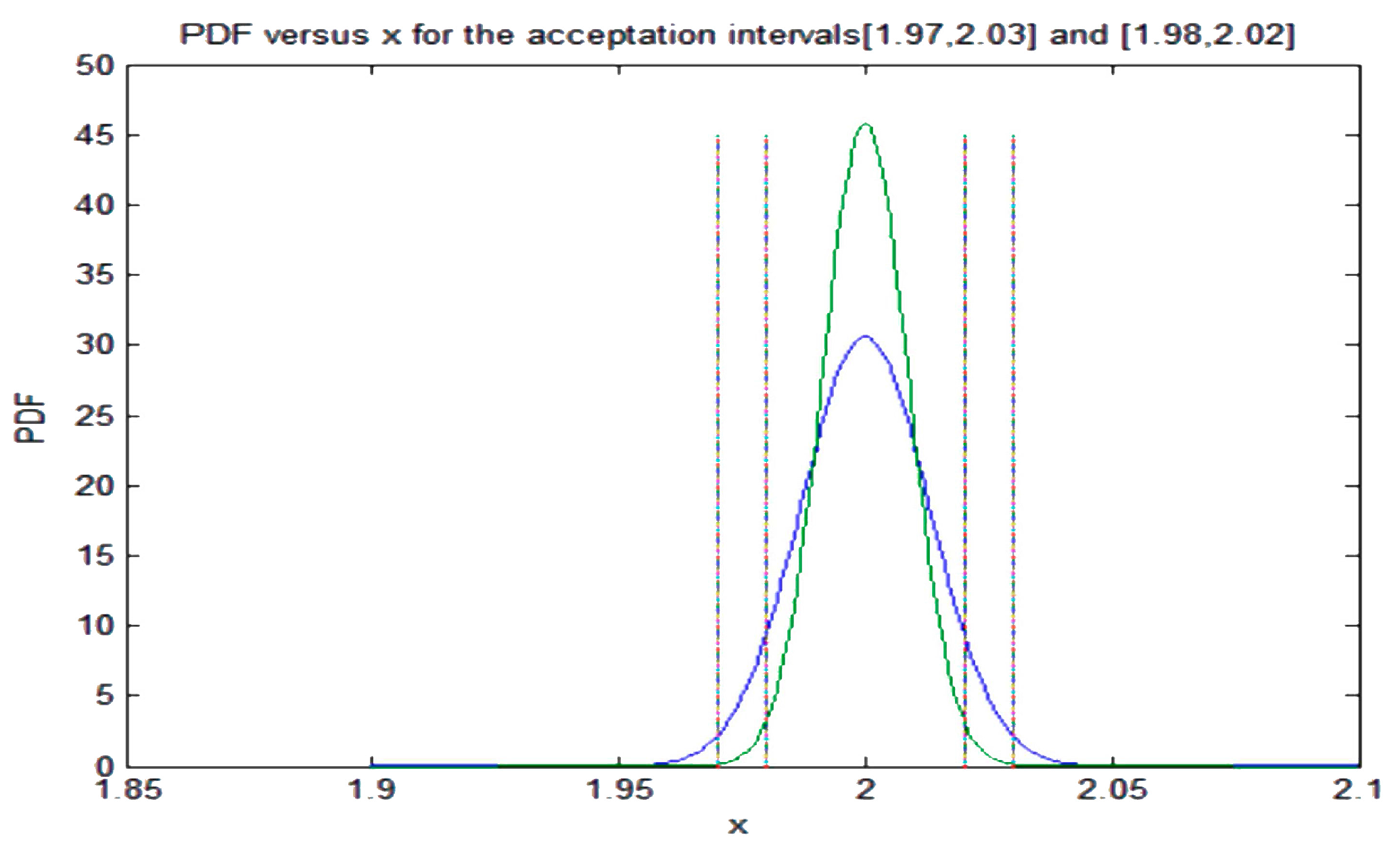
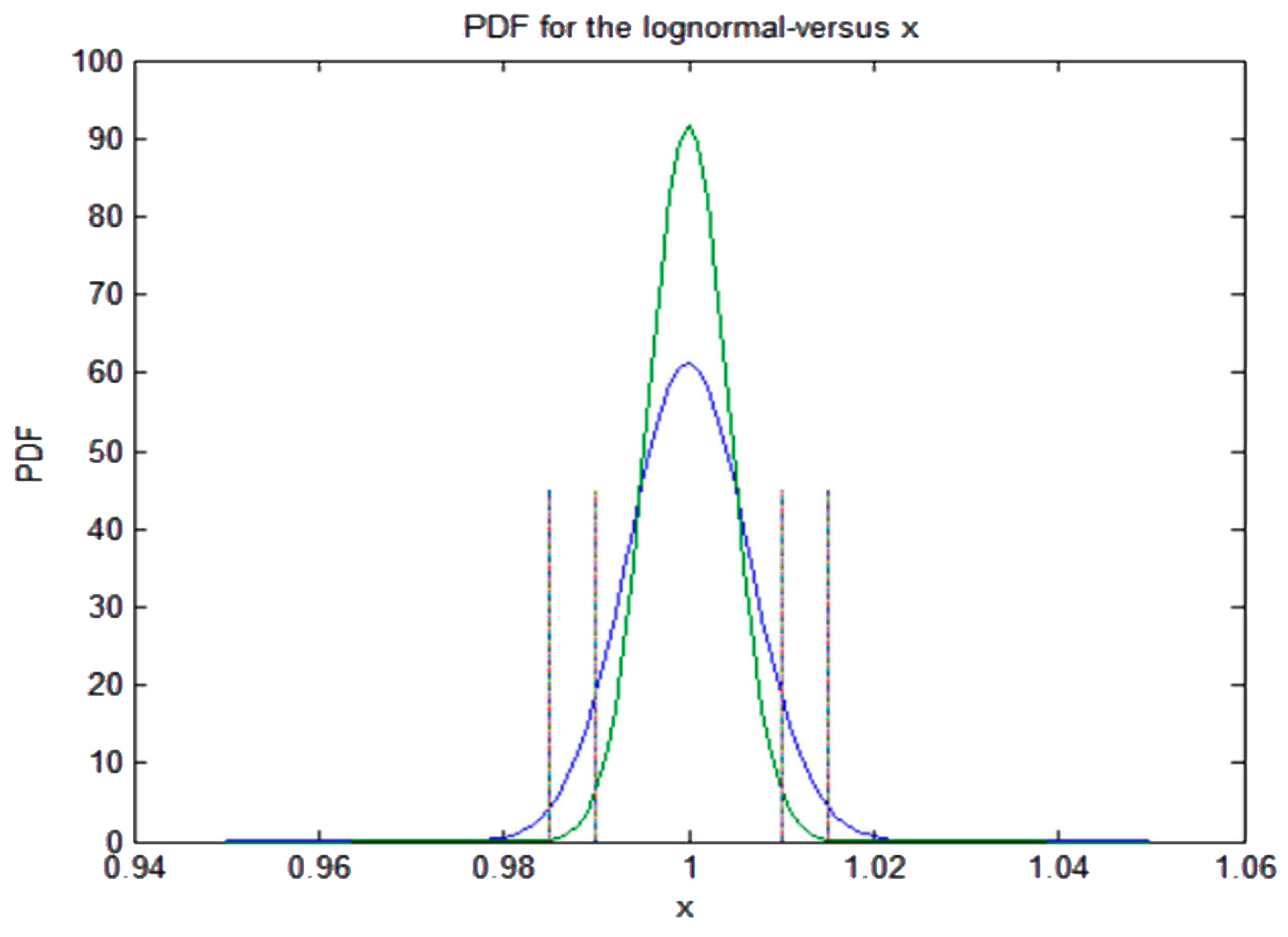
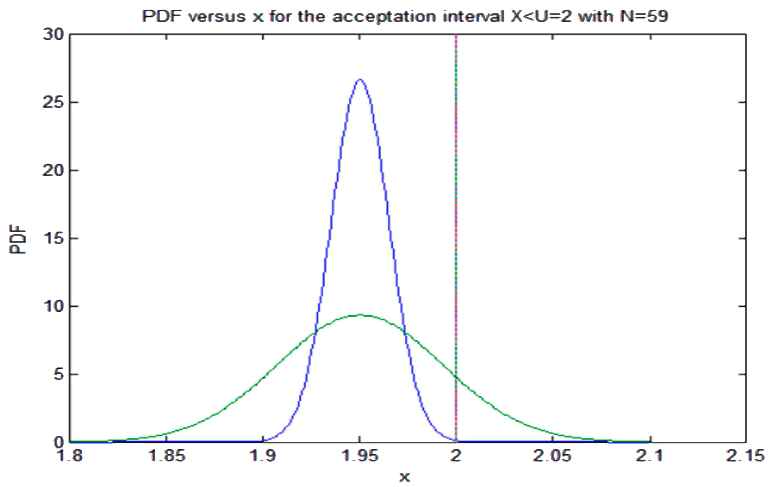
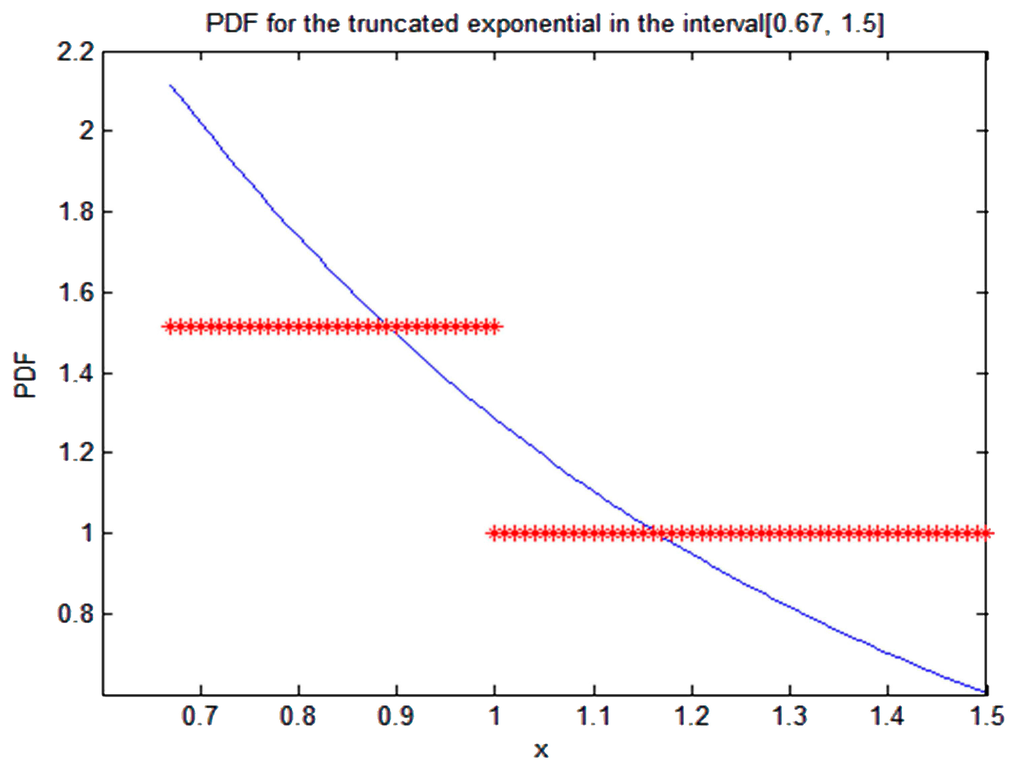
For instance, the solution of Equation (15) using the inverse of the incomplete beta function, i.e., “betaincinv” of MATLAB with N = 93, $\beta =0.95, M=⎡0.95 \times 93⎤=89$ gives p = 0.9786. Therefore, in this case, the additional restriction that we have on the PDF and that is imposed by the technical specification is

$$\underset{L}{\overset{U}{\int }}{q}_X\left(x\right)dx=p$$

(16)

The condition (16) can be expressed if the support of the distribution is $\left[a, b\right]$ as follows

$$\underset{a}{\overset{b}{\int }}{q}_X\left(x\right)\left[H\left(U-x\right)-H\left(L-x\right)\right]dx=p$$

(17)

where $H\left(U-x\right)$ is the Heaviside function that is zero for $x>U$, and 1 for the rest of values; $H\left(L-x\right)$ is the Heaviside function that is zero for $x>L$, and 1 for the rest of values.

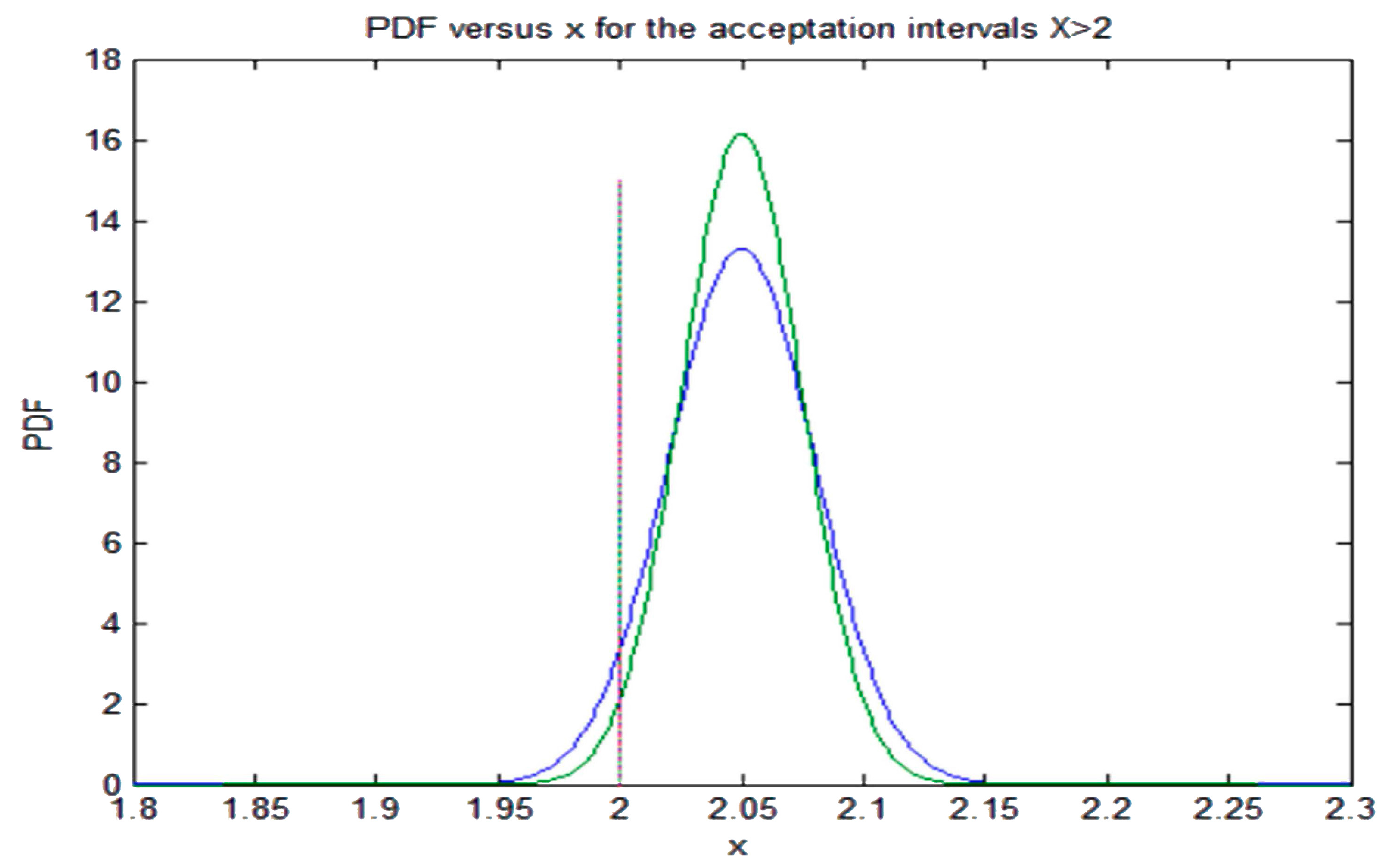
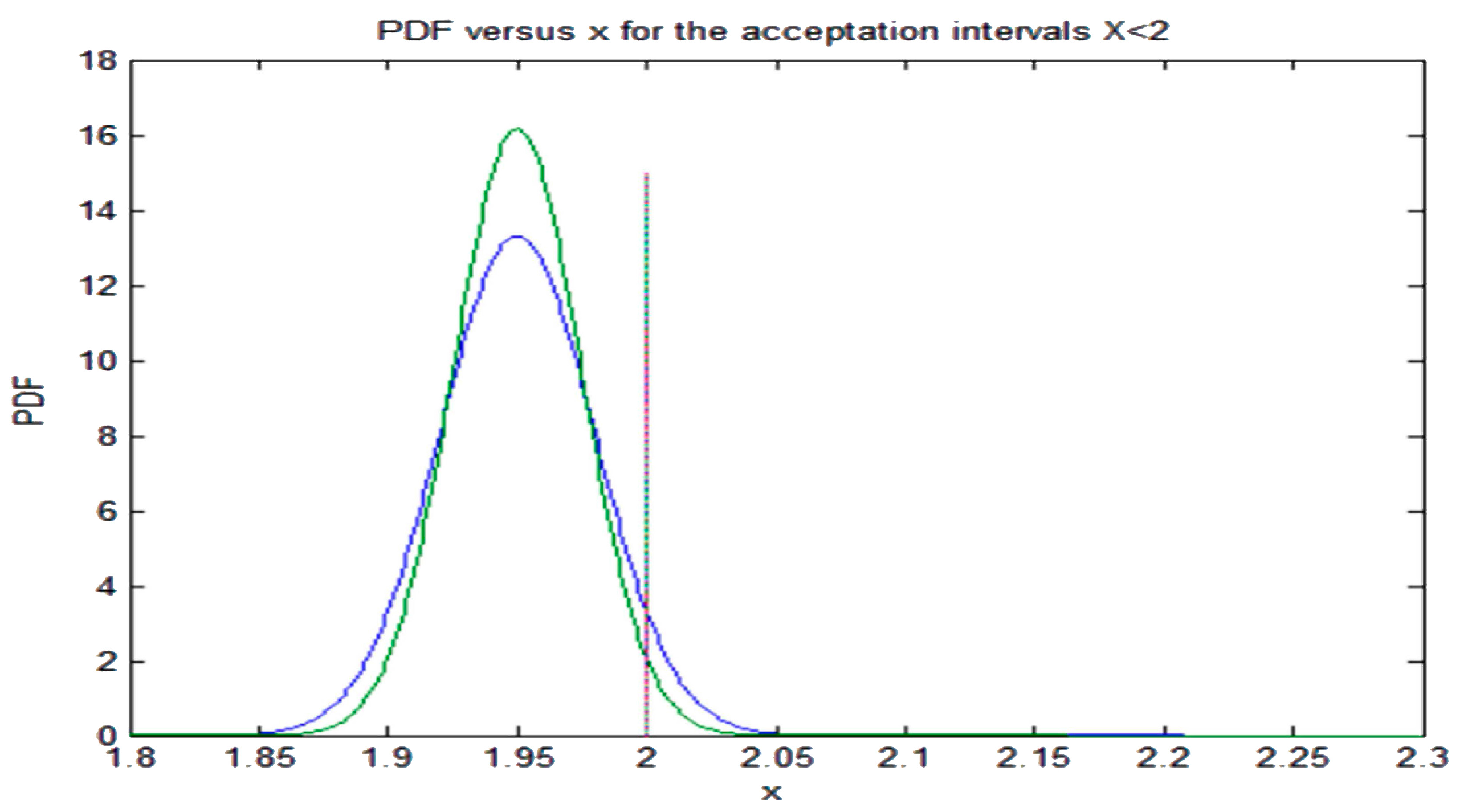
The question is that the TS through the surveillance and repairing actions modifies the parameter distribution in such a way that some parameter of the distribution could be modified to fulfill Equation (16), normally this parameter is the variance of the distribution that it is changed to comply with (16). The regulatory authority could modify the value of p given by (15) to perform a conservative analysis [22]. This last point will be discussed later in Section 5.4.3. Let us discuss the general conditions that must verify $q_X\left(x\right)$, first the function must be a continuous function in order to have an unambiguous probability value for each x, second for these kind of problems influenced by the TS, the average value of the distribution in general does not change for symmetrical distributions because this value represents the reference value of the TS—i.e., the reference pressure for opening or closing the valve—although this statement in some particular cases could change. Also, some moments such as the variance related to the width of the distribution could change. The way to proceed is as follows, first with the known support and the distribution moments we apply the MEP and we determine the previous probability distribution, $f_X\left(x\right).$ Second, we build the functional that considers the moments that can change as unknowns and take into account the TS condition (17) and the known moments

$$F\left(q_X,f_X\right)=-{\int }_a^{b}dx q_X\left(x\right)\log \left(\raisebox{1ex}{$q_X\left(x\right)$}\!\left/ \!\raisebox{-1ex}{$f_X\left(x\right)$}\right.\right)+{\displaystyle \sum }_{i=0}^n{\lambda }_i^{\prime }\left[{\int }_a^b{g}_i\left(x\right)q_X\left(x\right)-{\mu }_i^{\prime }\right]+{\lambda }_{n+1}^{\prime }\left[{\int }_a^{b}dx{q}_X\left(x\right)\left(H\left(U-x\right)-H\left(L-x\right)\right)-p\right]$$

(18)

Proceeding as in the previous subsection—i.e., equating to zero the first variation—yields the following expression for the new PDF that considers the TS and maximizes the relative entropy

$$q_X\left(x\right)=f_X\left(x\right)\exp \left\{-1+{\displaystyle \sum }_{i=0}^n{\lambda }_i^{\prime }{g}_i\left(x\right)+{\lambda }_{n+1}^{\prime }\left(H\left(U-x\right)-H\left(L-x\right)\right)\right\}$$

(19)

The unknown parameter values of the new PDF are obtained from the updated conditions (11), the TS condition (16), and the continuity of $q_X\left(x\right)$ at $L$ and $U$. Some examples will be shown in the next section.

4. Examples of Application of the MEP and the MREP to the Determination of the PDF of Parameters with and without Technical Specifications

4.1. Application of the MEP and the MREP to the Case of Known Support $\left[-\infty ,\infty \right]$ and Previously Known Mean $\mu$, and Variance ${\sigma }^2$ When the TS Impose an Acceptance Interval $\left[L,U\right]$ with Coverage $\gamma$ and Confidence $\beta$

This case appears sometimes during the application of BEPU methodologies. These methodologies, first at all, determine the number of cases N to be run by the code by the Wilks formula [28,29], that depends on the coverage and the confidence levels in (3), normally 95/95 for the output variable. Once N is known, each input or model parameter of the code that is important in the output response for the critical safety parameter must be randomly sampled N times over its distribution. Then, we generate N data sets by Monte Carlo sampling over the PDF that follows each individual parameter. Each data set contains a set of input parameters and the code is executed N times with each one of these data sets. From the output results of the code, it is easy by order statistic methods to build a tolerance interval for the desired output variable with a coverage ${\gamma }_0$ and a confidence ${\beta }_0$. Note that this coverage and confidence for the output variable of the code are not necessary the same that for the input parameter data.

It is easy to prove that if the random parameter has the support $\left[-\infty , \infty \right]$, mean $\mu$, and variance ${\sigma }^2$, then the application of the MEP leads to a Gaussian distribution [5], see also Appendix B

$$f_X\left(x\right)=\frac{1}{\sqrt{2\pi }\sigma }\exp \left(-\frac{1}{2}{\left(\frac{x-\mu }{\sigma }\right)}^2\right)$$

(20)

Let us assume that when performing the sampling of the parameter we want that the parameter complies the TS with a probabilistic criterion without changing the average value $\mu$ that is normally related to the reference value of the TS. In addition, because we are applying a Wilks’ methodology with N cases, we want that at least $M=\lceil \gamma \hspace{0.17em}N\rceil$ values of the parameter belong to the acceptance interval $\left[L, U\right]$ with confidence $\beta$. Therefore, the new probability density function $q_X\left(x\right)$ of the parameter must verify the condition

$$\underset{L}{\overset{U}{\int }}{q}_X\left(x\right)dx=\underset{-\infty }{\overset{+\infty }{\int }}{q}_X\left(x\right)\left[H\left(U-x\right) - H\left(L - x\right)\right]dx=p$$

(21)

While, as explained in Appendix A, $p$ is obtained solving Equation (15). In addition, $q_X\left(x\right)$ must verify the following set of conditions

$$\underset{-\infty }{\overset{+\infty }{\int }}{q}_X\left(x\right)dx=1; {\int }_{-\infty }^{+\infty }x{q}_X\left(x\right)dx=\mu ; {\int }_{-\infty }^{+\infty }{\left(x-\mu \right)}^2{q}_X\left(x\right)dx={\sigma }^{\prime }{}^2\ne {\sigma }^2$$

(22)

The value of the new unknown parameter ${\sigma }^{\prime }{}^2$ and the new distribution function will be obtained applying the MREP, with the previously known PDF $f_X$(x) as weighting or ranking reference once we know the value of p that it is obtained by solving Equation (15), or has been set by the regulatory body. The new function that contains the relative entropy and the set of restriction conditions is given by

$$F\left(q_X,f_X\right)=-{\int }_{-\infty }^{+\infty }dx q_X\left(x\right)\log \left(\raisebox{1ex}{$q_X\left(x\right)$}\!\left/ \!\raisebox{-1ex}{$f_X\left(x\right)$}\right.\right)+{\lambda }_0^{\prime }\left[{\int }_{-\infty }^{+\infty }dx{q}_X\left(x\right)-1\right]+{\lambda }_1^{\prime }\left[{\int }_{-\infty }^{+\infty }dxx{q}_X\left(x\right) - \mu \right]+{\lambda }_2^{\prime }\left[{\int }_{-\infty }^{+\infty }dx{\left(x-\mu \right)}^2{q}_X\left(x\right) - {\sigma \prime }^2\right]+{\lambda }_3^{\prime }\left[{\int }_a^{b}dx{q}_X\left(x\right)\left(H\left(U - x\right) - H\left(L - x\right)\right) - p\right]$$

(23)

Then, we equate to zero the first variation of (23), i.e., we set $\delta F\left(q_X,f_X\right)=0$, and after some calculus the following result is obtained for the new PDF that maximizes the relative entropy

$$q_X\left(x\right)=f_X\left(x\right)\exp \left(-1+{\lambda }_0^{\prime }+{\lambda }_1^{\prime }x+{\lambda }_2^{\prime }{\left(x-\mu \right)}^2+{\lambda }_3^{\prime }\left(H\left(U - x\right) - H\left(L - x\right)\right)\right)$$

(24)

The PDF given by Equation (24) must satisfy the conditions (21) and (22). Notice that inside the acceptance interval [L, U] the difference of the Heaviside function is 1 and outside [L, U] is zero. Therefore, Equation (24) can be expressed in the form

$$q_X\left(x\right)=f_X\left(x\right)\mathrm{D}\exp ({\lambda }_1^{\prime }x+{\lambda }_2^{\prime }{\left(x - \mu \right)}^2), if x\notin \left[L,U\right]$$

(25)

$$q_X\left(x\right)=f_X\left(x\right)D^{\prime }\exp ({\lambda }_1^{\prime }x+{\lambda }_2^{\prime }{\left(x - \mu \right)}^2), if x\in \left[L,U\right]$$

(26)

where the new constants $D$ and $D^{\prime }$ are given by the expressions

$$D=\exp \left(-1+{\lambda }_0^{\prime }\right) \mathrm{and} D=\exp \left(-1+{\lambda }_0^{\prime }+{\lambda }_3^{\prime }\right)$$

(27)

From the continuity of the PDF $q_X\left(x\right)$, at x = $L$ or x = $U$, it is obtained that $D=D^{\prime }$. From this condition, it is deduced that

$$\exp \left({\lambda }_3^{\prime }\right)=1\stackrel{yields}{\to }{\lambda }_3^{\prime }=0$$

(28)

Therefore, the new updated PDF that fulfills the TS is given, because of (20), (24), (27), and (28), by

$$q_X\left(x\right)=\frac{1}{\sqrt{2\pi }\sigma }D \exp \left\{{\lambda }_1^{\prime }x+{\lambda }_2^{\prime }{\left(x - \mu \right)}^2 - \frac{1}{2}{\left(\frac{x - \mu }{\sigma }\right)}^2\right\}$$

(29)

Next, we consider that the PDF given by (29) must satisfy Equation (21) and the set of Equation (22). In this case, we have assumed that the TS does not change the reference value, for instance, the reference pressures to open the safety and relief valve, but the limitation imposed by the TS in Equation (21) is more restrictive and could change the variance of the distribution. Then, Equation (22) because of Equation (29) yield the following set of conditions

$$\underset{-\infty }{\overset{+\infty }{\int }}dx\frac{1}{\sqrt{2\pi }\sigma }D \exp \left\{{\lambda }_1^{\prime }x+{\lambda }_2^{\prime }{\left(x - \mu \right)}^2 - \frac{1}{2}{\left(\frac{x - \mu }{\sigma }\right)}^2\right\}=1$$

(30)

$$\underset{-\infty }{\overset{+\infty }{\int }}dx x\frac{1}{\sqrt{2\pi }\sigma }D \exp \left\{{\lambda }_1^{\prime }x+{\lambda }_2^{\prime }{\left(x - \mu \right)}^2 - \frac{1}{2}{\left(\frac{x - \mu }{\sigma }\right)}^2\right\}=\mu$$

(31)

$$\underset{-\infty }{\overset{+\infty }{\int }}dx {\left(x - \mu \right)}^2\frac{1}{\sqrt{2\pi }\sigma }D \exp \left\{{\lambda }_1^{\prime }x+{\lambda }_2^{\prime }{\left(x - \mu \right)}^2 - \frac{1}{2}{\left(\frac{x - \mu }{\sigma }\right)}^2\right\}={\sigma }^{\prime }{}^2\ne {\sigma }^2$$

(32)

Together with Equation (21), written in the form

$${\int }_L^{U}dx q_X\left(x;\mathsf{\Theta }\right)=F_X\left(U;\mathsf{\Theta }\right) - F_X\left(L;\mathsf{\Theta }\right)=p$$

(33)

where $\mathsf{\Theta }$ denotes the set of parameters values that determine the distribution function and that normally depend on the type of distribution, for instance for a Gaussian these parameters are the mean and the variance. $F_X\left(U;\Theta \right)$ is the cumulative distribution function (CDF) evaluated at the upper limit U of the acceptance interval, while $F_X\left(L;\Theta \right)$ is the CDF evaluated at the lower limit L of the acceptance interval.

Then, Equation (31) can be written as

$$\underset{-\infty }{\overset{+\infty }{\int }}dxx\frac{1}{\sqrt{2\pi }\sigma }D\exp \left\{{\lambda }_1^{\prime }x+\left({\lambda }_2^{\prime }-\frac{1}{2{\sigma }^2}\right){\left(x-\mu \right)}^2\right\}=\mu$$

(34)

With the change of variables $x - \mu =t$, we can express Equation (34) in the form

$$\underset{-\infty }{\overset{+\infty }{\int }}dt\left(t+\mu \right)\frac{1}{\sqrt{2\pi }\sigma }D\exp \left\{{\lambda }_1^{\prime }\left(t+\mu \right)+\left({\lambda }_2^{\prime }-\frac{1}{2{\sigma }^2}\right)t^2\right\}=\mu$$

(35)

Next because condition (30), Equation (35) simplifies to

$$\underset{-\infty }{\overset{+\infty }{\int }}dtt\exp \left\{{\lambda }_1^{\prime }\left(t+\mu \right)+{\lambda }_3^{\prime }{t}^2\right\}=0$$

(36)

where ${\lambda }_3^{\prime }=\left({\lambda }_2^{\prime } - \frac{1}{2{\sigma }^2}\right)$. Because $\exp \left({\lambda }_3^{\prime }{t}^2\right)$ is an even function ($f\left(-t\right)=f\left(t\right))$ and t is an odd function ($f\left(-t\right)=-f\left(t\right))$, then it follows that, in order that the integral (36) vanishes, the Lagrange multiplier ${\lambda }_1^{\prime }$ must be equal to zero.

The coefficient $D$ can be now calculated from (30), on account of ${\lambda }_1^{\prime }=0$

$$\underset{-\infty }{\overset{+\infty }{\int }}dx\frac{1}{\sqrt{2\pi }\sigma }D \exp \{{\lambda }_3^{\prime }{\left(x-\mu \right)}^2\}=\underset{-\infty }{\overset{+\infty }{\int }}dt\frac{1}{\sqrt{2\pi }\sigma }D \exp \left\{{\lambda }_3^{\prime }{t}^2\right\}=\frac{1}{\sqrt{2\pi }\sigma }D \sqrt{\frac{\pi }{-{\lambda }_3^{\prime }}}=1$$

(37)

Therefore, the coefficient $D$ is given by the expression

$$D=\sigma \sqrt{-2{\lambda }_3^{\prime }}$$

(38)

To compute the value of ${\lambda }_3^{\prime }$ we use condition (32), because (38), performing the change of variables $x - \mu =t$ and the integral in (32), gives after some calculus

$$\underset{-\infty }{\overset{+\infty }{\int }}dx t^2\frac{1}{\sqrt{2\pi }\sigma }D \exp \left\{{\lambda }_3^{\prime }{t}^2\right\}=\frac{1}{\sqrt{2\pi }\sigma }D\frac{1}{2\left(-{\lambda }_3^{\prime }\right)}\sqrt{\frac{\pi }{-{\lambda }_3^{\prime }}}={\sigma }^{\prime }{}^2$$

(39)

From Equations (38) and (39), it is deduced that

$${\lambda }_3^{\prime }=-\frac{1}{2{\sigma }^{\prime }{}^2}$$

(40)

Finally, after some trivial algebra, one arrives at the expression of the PDF $q_X\left(x;\Theta \right)$ that considers the technical specifications

$$q_X\left(x;\Theta \right)=\frac{1}{\sqrt{2\pi }{\sigma }^{\prime }}\exp \left(-\frac{1}{2}{\left(\frac{x - \mu }{{\sigma }^{\prime }}\right)}^2\right)$$

(41)

Once we know the PDF type, we must obtain the unknown parameter value ${\sigma }^{\prime }$, that in this case is obtained solving the Equation (33), and looking for the value of ${\sigma }^{\prime }$ such that the integral of the PDF over the acceptance interval yields the probability p, that is obtained from (15). Then we will display some calculations about this type of problem and their applications.

4.2. Application of the Principle of MRE to Cases with Previously Known Distributions When New Information is Known without and with Technical Specifications

Some examples of parameter distribution updating are showed in this section. The updating with the new information is performed using the maximum relative entropy principle. The entropy in this case is ranked with respect to the previously known distribution, as explained in the previous section.

4.2.1. Application of the MRE Principle to the Case of a Parameter with Previously Uniform Distribution in the Interval [a, b], and the New Information Available is the Parameter Mean Value $\mu$

A common case for many parameters is to use a uniform distribution when their distributions are unknown. As it is well known, uniform distribution maximizes the entropy in the interval [a, b] when we do not have more information. This is the reason why in many BEPU analysis methodologies it is assumed that many parameters follow the uniform distribution [30]. Let us assume that the previous or ‘prior’ parameter distribution is the uniform one, given by

$$f_X\left(x\right)=\{\begin{array}{c}\frac{1}{b - a}, for a\le x\le b\\ 0, for x\notin \left[a, b\right]\end{array}$$

(42)

If we know new information on the parameters, for instance the mean value $\mu$, then we can use the MRE principle to update the PDF with this information, as explained in Section 3. Then, if it is assumed that the distribution support does not change, it is obtained because Equation (14) the following result for the updated PDF

$$q_X\left(x\right)=\{\begin{array}{c}\frac{1}{b-a}\exp \left\{-1+{\lambda }_0^{\prime }+{\lambda }_1^{\prime }x\right\}=\frac{1}{b-a}D\exp \left\{{\lambda }_1^{\prime }x\right\}, for a\le x\le b \\ 0 , for x\notin \left[a, b\right]\end{array}$$

(43)

In this case, the application of the normalization condition gives

$$\underset{a}{\overset{b}{\int }}\frac{1}{b-a}D \exp \left\{{\lambda }_1^{\prime }x\right\}dx=1\stackrel{yields}{\Rightarrow }D=\frac{{\lambda }_1^{\prime }\left(b-a\right)}{\exp \left({\lambda }_1^{\prime }b\right)-\exp \left({\lambda }_1^{\prime }a\right)}$$

(44)

Then, because of Equations (43) and (44), it is obtained that the updated PDF $q_X\left(x\right)$ is the following truncated exponential

$$q_X\left(x\right)=\{\begin{array}{c}\frac{{\lambda }_1^{\prime }}{\exp \left({\lambda }_1^{\prime }b\right)-\exp \left({\lambda }_1^{\prime }a\right)}\exp \left\{{\lambda }_1^{\prime }x\right\}, for a\le x\le b \\ 0 , for x\notin \left[a, b\right]\end{array}$$

(45)

The value of the parameter ${\lambda }_1^{\prime }$ is obtained from the first moment condition that can be expressed as follows

$$\underset{a}{\overset{b}{\int }}x{q}_X\left(x\right)dx=\frac{{\lambda }_1^{\prime }}{\exp \left({\lambda }_1^{\prime }b\right)-\exp \left({\lambda }_1^{\prime }a\right)}\underset{a}{\overset{b}{\int }}x\exp \left\{{\lambda }_1^{\prime }x\right\}dx=\mu$$

(46)

Performing by parts the integral that appears in Equation (46) yields the following equation that must be solved to obtain the unknown Lagrange multiplier ${\lambda }_1^{\prime }$

$$\frac{b\exp \left({\lambda }_1^{\prime }b\right)-a\exp \left({\lambda }_1^{\prime }a\right)}{\exp \left({\lambda }_1^{\prime }b\right)-\exp \left({\lambda }_1^{\prime }a\right)}-\frac{1}{{\lambda }_1^{\prime }}=\mu$$

(47)

The unknown value of the Lagrange multiplier ${\lambda }_1^{\prime }$ depends on, $b$, and $\mu$, and must be obtained solving the non-linear Equation (47). For the case of $a=-1$ and $b=1$, the Equation (47) simplifies to

$$\coth \left({\lambda }_1^{\prime }\right)-\frac{1}{{\lambda }_1^{\prime }}=\mu$$

(48)

Representing the $\mu$ at the y axis versus the ${\lambda }_1^{\prime }$ at the x axis it is obtained the plot displayed at Figure 1. When ${\lambda }_1^{\prime }\to 0$ it is obtained that $\mu \to 0$ and reciprocally as it is easily checked. This means that when the parameter ${\lambda }_1^{\prime }$ tends toward zero, the distribution becomes uniform in the interval [−1, 1] and, therefore, the average value $\mu$ is zero. The reciprocal is also simple, if $\mu \to 0$ then it follows from Equation (48) that $tanh\left({\lambda }_1^{\prime }\right)={\lambda }_1^{\prime }$ and therefore ${\lambda }_1^{\prime }=0$.

4.2.2. Application of the MREP to the Case of a Parameter with Previously Truncated Exponential Distribution in the Interval [a, b] with Mean Value $\mu$, and the New Parameter Mean Value $\mu$ is the Same and the TS Impose an Acceptance Interval [L, U]

In this case, the previous distribution is the truncated exponential given by Equation (45). Now, the TS impose an acceptance interval [L, U] and the new probability density function $q_X\left(x\right)$ of the parameter must verify the condition (21) being the mean value $\mu$ the same. Then, the only degree of freedom of the distribution is its support that is adjusted to comply the TS. Applying the MREP, and after some calculations, we obtain

$$q_X\left(x\right)=\{\begin{array}{c}\frac{{\lambda }_1^{″}}{\exp \left({\lambda }_1^{″}{b}^{\prime }\right)-\exp \left({\lambda }_1^{″}{a}^{\prime }\right)}\exp \left\{{{\lambda }^{\prime }}_1^{\prime }x\right\}, for a^{\prime }\le x\le b^{\prime } \\ 0 , for x\notin \left[a^{\prime },b^{\prime }\right]\end{array}$$

(49)

The new limits $a\prime$ and $b\prime$ are unknown. The condition for the first moment of the distribution is

$$\underset{a^{\prime }}{\overset{b^{\prime }}{\int }}x{q}_X\left(x\right)dx=\frac{{\lambda }_1^{″}}{\exp \left({\lambda }_1^{″}{b}^{\prime }\right)-\exp \left({\lambda }_1^{″}{a}^{\prime }\right)}\underset{a^{\prime }}{\overset{b^{\prime }}{\int }}x\exp \left\{{\lambda }_1^{″}x\right\}dx=\mu$$

(50)

Equation (50) yields the following equation that must be solved to obtain the unknown value of the Lagrange multiplier ${\lambda }_1^{″}$ once a′ and $b\prime$ are known

$$\frac{b^{\prime }\exp \left({\lambda }_1^{″}{b}^{\prime }\right)-a^{\prime }\exp \left({\lambda }_1^{″}{a}^{\prime }\right)}{\exp \left({\lambda }_1^{″}{b}^{\prime }\right)-\exp \left({\lambda }_1^{″}{a}^{\prime }\right)}-\frac{1}{{\lambda }_1^{″}}=\mu$$

(51)

However, the inconvenience is that $a\prime$ and $b\prime$ are unknown. Without loss of generality, let us assume that the mean value is in the center of the support [$a\prime$,$b\prime$]. For this case, if t denotes the half width of the interval [$a\prime$,$b\prime$], then we may write $a^{\prime }=\mu - t$,$b^{\prime }=\mu + t$, substitution of these values into Equation (51) gives the following equation

$${\lambda }_1^{″}t \coth \left({\lambda }_1^{″}t\right)=1$$

(52)

The only solution of this equation is ${\lambda }_1^{″}t=0,$ so we have that ${\lambda }_1^{″}=0$, i.e., we have a uniform distribution. Applying the condition (21) imposed by the TS, and denoting the half width of the acceptance interval by s, we have

$$\underset{L}{\overset{U}{\int }}{q}_X\left(x\right)dx=\frac{U - L}{b^{\prime } - a^{\prime }}=\frac{2s}{2t}=p$$

(53)

Because $p$ is known, as was explained in Section 3.3, and s is also known because is given by the TS, then we can obtain directly a′ and b′. For the example of Section 5.2, with N = 93 and coverage and confidence 95/95 then p = 0.9786. Therefore, because in this example $U=p_{ref} + 0.015 p_{ref}$ and $L=p_{ref}-0.015p_{ref}$, from Equation (53) it is deduced that $t=0.015328 p_{ref}.$ Because we have assumed that $\mu$ is in the center of [$a\prime$, $b\prime$], then it follows $a^{\prime }=\mu - 0.015328 p_{ref}$ and $b^{\prime }=\mu +0.015328 p_{ref}$. As a conclusion of this subsection, to fulfill the TS the half-width of the distribution, t, should be modified to verify the condition (53).

4.3. Application of the MREP to the Case of a Parameter with Previously Truncated Gaussian Distribution in the Interval [a, b] with Mean Value $\mu =\left(a+b\right)/2$, and Variance ${\sigma }^2$, the Updated Data Have the Same Support, the Same $\mu$ But Different Variance ${\sigma }^{\prime }{}^2$

The Gaussian truncated distribution is used when sampling over distributions that have an upper and a lower limit for the parameter X and the available information is the mean and the variance. In this case, it is common to perform the following change of variables $z=\left(x - \mu \right)/s$, where s = (b − a)/2 is the half width of the distribution, and the relation between both PDF is $f_X\left(x\right)=\frac{1}{s}{f}_Z\left(\frac{x-\mu }{s}\right)$. Thus, the random variable Z distributes in the interval [−1, 1].

The application of the MEP with the restrictions due to the previous information (the mean and the variance) yields the following result for the previous PDF, as shown by Muñoz-Cobo et al. [5] and Udwadia [16]

$$f_Z\left(z\right)=\{\begin{array}{c}D\exp \left( {\lambda }^{\prime }{z}^2\right) for-1\le z\le 1\\ 0, for z\notin \left[-1, 1\right]\end{array}$$

(54)

The value of the parameter ${\lambda }^{\prime }$ is obtained solving the following equation

$${\left(\frac{\sigma }{s}\right)}^2=\frac{\log (0.5{\int }_{-1}^{1}dz \exp \left({\lambda }^{\prime }{z}^2\right))}{{\lambda }^{\prime }}$$

(55)

Usually, we know $\sigma$ and the half width s, so we can plot $\frac{\sigma }{s}$ versus ${\lambda }^{\prime }$, this gives the graphic displayed at Figure 2. From the plot, it is very easy to obtain the value of ${\lambda }^{\prime }$ corresponding to a given $\frac{\sigma }{s}$ value.

Table 1. $\raisebox{1ex}{$\mathsf{\sigma }$}\!\left/ \!\raisebox{-1ex}{$\mathrm{s}$}\right.$ and ${\lambda }^{\prime }$ for negative ${\lambda }^{\prime }$ values.

${\mathit{\lambda }}^{\prime }$	−10	−9	−8	−7	−6	−5	−4	−3	−2	−1	−0.5
$\frac{\sigma }{s}$	0.3567	0.3681	0.3809	0.3953	0.4117	0.4306	0.4524	0.4776	0.5069	0.5401	0.5578
${\lambda }^{\prime }$	−80	−60	−40	−35	−30	−20	−18	−16	−14	−12
$\frac{\sigma }{s}$	0.1700	0.1901	0.2217	0.2329	0.2464	0.2845	0.2950	0.3069	0.3207	0.3371

shows the values of $\sigma /s$ corresponding to the negative integer values of ${\lambda }^{\prime }$ ranging from −1 to −80.

Once we have computed the value of the parameter ${\lambda }^{\prime }$, the value of the constant $D$ in Equation (54) is obtained from the normalization condition of the PDF. This calculation yields

$$D=\frac{1}{{\int }_{-1}^{1}dx \exp \left({\lambda }^{\prime }{x}^2\right)}=\frac{1}{\sqrt{\frac{\pi }{-{\lambda }^{\prime }}}\mathrm{erf}\left(\sqrt{-{\lambda }^{\prime }}\right)}$$

(56)

Being $\mathrm{erf}(\sqrt{-{\lambda }^{\prime }}$) the error function evaluated at $\sqrt{-{\lambda }^{\prime }}$.

Figure 3 displays the truncated Gaussian evaluated for the following negative lambda values ${\lambda }^{\prime }=-10, -9, -8,-7,-6,-5,-4,-3,-2,-1,-0.5$. As observed in Table 1, the values of $\sigma$ increase when ${\lambda }^{\prime }$ increases from −10 to −0.5.

To get the updated PDF, assuming that the support [a, b] and the mean $\mu =\frac{a+b}{2}$ are the same as in the previous PDF, and the variance change from $\sigma$ to ${\sigma }^{\prime }$, we proceed as follows: first we know that the previous PDF was $f_X\left(x\right)=\frac{1}{s}{f}_Z\left(\frac{x-\mu }{s}\right)$ that was obtained by application of the MEP. Then to apply the principle of the maximum relative entropy with the new restrictions, and considering that the new probability distribution $q_X\left(x\right)$ should be ranked according to its relative entropy with respect to the previously known PDF $f_X\left(x\right)$, we built the following functional

$$F\left(q_X,f_X\right)=-\underset{a}{\overset{b}{\int }}dx{q}_X\left(x\right)\log \left(\frac{q_X\left(x\right)}{f_X\left(x\right)}\right)+{\lambda }_0^{\prime }\left[\underset{a}{\overset{b}{\int }}dx{q}_X\left(x\right)-1\right]+{\lambda }_1^{\prime }\left[\underset{a}{\overset{b}{\int }}dxx{q}_X\left(x\right)-\mu \right]+{\lambda }_1^{\prime }\left[\underset{a}{\overset{b}{\int }}dx{\left(x-\mu \right)}^2{q}_X\left(x\right)-{\sigma }^{\prime }{}^2\right]$$

(57)

Setting to zero the first variation $\delta F=0$ it is obtained, after some calculus and simplifications, the following result for the updated PDF $q_X\left(x\right)$

$$q_X\left(x\right)=f_X\left(x\right)D^{\prime }\exp ({\lambda }_1^{\prime }x+{\lambda }_2^{\prime }{\left(x-\mu \right)}^2),ifx\in \left[a,b\right]$$

(58)

$$q_X\left(x\right)=0,ifx\notin \left[a,b\right]$$

(59)

Because Expression (53) for the previous PDF, it is deduced that the updated PDF can be written, after performing some trivial manipulations

$$q_X\left(x\right)=D^{″}\exp ({\lambda }_1^{″}x+{\lambda }_2^{″}{\left(x-\mu \right)}^2),ifx\in \left[a,b\right]$$

(60)

From the condition ${\int }_a^{b}dxx{q}_X\left(x\right)=\mu$, it is easy to prove, as was done in previous sections, that the parameter ${\lambda }_1^{″}=0$. The constants $D^{″}$ and ${\lambda }_2^{″}$ should be obtained from the rest of new moment restrictions.

Performing the change of variables $z=\left(x-\mu \right)/s$, where s = (b − a)/2 and $x=zs+\mu$, it is obtained that the updated PDF, expressed in terms of z, is given by the expression

$$q_Z\left(z\right)=\{\begin{array}{c}{D}^{‴}\exp \left({\lambda }^{‴}{z}^2\right) for-1\le z\le 1\\ 0, for z\notin \left[-1, 1\right]\end{array}$$

(61)

where we have set $D^{‴}=s{D}^{″}$ and ${\lambda }^{‴}={\lambda }_2^{″}{s}^2$, and from the normalization condition of the PDF it follows that

$$D^{‴}=\frac{1}{{\int }_{-1}^{1}dz\exp \left({\lambda }^{‴}{z}^2\right)}=\frac{1}{\sqrt{\frac{\pi }{-{\lambda }^{‴}}}\mathrm{erf}\left(\sqrt{-{\lambda }^{‴}}\right)}$$

(62)

To find the ${\lambda }^{‴}$ value, we use the second moment restriction, after performing the change of variables from $x$ to $z,$ it yields

$$\underset{-1}{\overset{1}{\int }}dz{z}^2{D}^{‴}\exp \left({\lambda }^{‴}{z}^2\right)={\left(\frac{{\sigma }^{\prime }}{s}\right)}^2$$

(63)

To solve this equation, one considers the parametric integral $I\left({\lambda }^{‴}\right)=\underset{-1}{\overset{1}{\int }}dz \exp \left({\lambda }^{‴}{z}^2\right)$ that depends on the $$ parameter. The derivation of this integral with respect to ${\lambda }^{‴}$ yields, because (63) and (64)

$$\frac{dI\left({\lambda }^{‴}\right)}{d{\lambda }^{‴}}=\underset{-1}{\overset{1}{\int }}dz{z}^2\exp \left({\lambda }^{‴}{z}^2\right)={\left(\frac{{\sigma }^{\prime }}{s}\right)}^2{\left(D^{‴}\right)}^{-1}=I\left({\lambda }^{‴}\right){\left(\frac{{\sigma }^{\prime }}{s}\right)}^2$$

(64)

The boundary condition to integrate Equation (64) is deduced from $I\left({\lambda }^{‴}=0\right)={\int }_{-1}^{1}dz=2$. Therefore, we have

$$I\left({\lambda }^{‴}\right)=2\exp \left({\left(\frac{{\sigma }^{\prime }}{s}\right)}^2{\lambda }^{‴}\right)={\left(D^{‴}\right)}^{-1}=\underset{-1}{\overset{1}{\int }}dz\exp \left({\lambda }^{‴}{z}^2\right)$$

(65)

So, to obtain ${\lambda }^{‴}$ one must solve the equation

$$\frac{\log \left(0.5{\int }_{-1}^{1}dz\exp \left({\lambda }^{‴}{z}^2\right)\right)}{{\lambda }^{‴}}={\left(\frac{{\sigma }^{\prime }}{s}\right)}^2$$

(66)

We observe that Equation (66) is the same one that Equation (55) with $\sigma$ changed by ${\sigma }^{\prime }\mathrm{and}{\lambda }^{\prime } by {\lambda }^{‴}$. For instance, changing the value of $\frac{\sigma }{s}=0.3953$ to $\frac{{\sigma }^{\prime }}{s}=0.4306$ produces a change in ${\lambda }^{‴}$ from −7 to −5.

4.4. Application of the MREP to the Case of a Parameter with Previously Log-Normal Distribution in the Interval (0, ∞) and New Measurements Yields $<logx>={\mu }_{log}$, Same Value as the Previous One and ${\left(log\left(x\right)-{\mu }_{log}\right)}^2={\sigma }^{\prime }{}^2$

Let us assume that the previous parameter distribution is a log-normal distribution, given as deduced by application of the MEP, sees Appendix B.2, by

$$f_X\left(x\right)=\frac{1}{\sqrt{2\pi }\sigma x}\exp \left(-\frac{1}{2}{\left(\frac{\log \left(x\right)-{\mu }_{\log }}{\sigma }\right)}^2\right)$$

(67)

Let us assume that new measurements yield $<\log \mathrm{x}>={\mu }_{log}$, and $<{\left(\log \left(x\right)-{\mu }_{log}\right)}^2>={\sigma }^{\prime }{}^2$. To update the PDF, on account of the previous distribution, we use the MREP. The first step is to build the following functional

$$F\left(q_X,f_X\right)=-{\int }_0^{+\infty }dx{q}_X\left(x\right)\log \left(\raisebox{1ex}{$q_X\left(x\right)$}\!\left/ \!\raisebox{-1ex}{$f_X\left(x\right)$}\right.\right)+{\lambda }_0^{\prime }\left[{\int }_0^{+\infty }dx{q}_X\left(x\right)-1\right]+{\lambda }_1^{\prime }\left[{\int }_0^{+\infty }dx\log (x)q_X\left(x\right)-{\mu }_{log}\right]+{\lambda }_2^{\prime }\left[{\int }_0^{+\infty }dx{\left(\log \left(x\right)-{\mu }_{log}\right)}^2{q}_X\left(x\right)-{\sigma }^{\prime }{}^2\right]$$

(68)

To update the PDF, we compute the first variation $\delta F=0$ and it is obtained, because Section 3.2, we get

$$q_X\left(x\right)=f_X\left(x\right)\exp (-1+{\lambda }_0+{\lambda }_1\log \left(x\right)+{\lambda }_2\left(\log \left(x\right)-{\mu }_{log}{)}^2\right)$$

(69)

Then, after some calculus, Equation (69) can be written, because Equation (67), as

$$q_X\left(x\right)=D{x}^{{\lambda }_1-1}\exp \left(\left({\lambda }_2-\frac{1}{2{\sigma }^2}\right){\left(\log \left(x\right)-{\mu }_{log}\right)}^2\right)$$

(70)

The next step is to use the condition ${\int }_0^{+\infty }dx\log (x)q_X\left(x\right)-{\mu }_{log}=0$, and to perform the change of variables $z=\log \left(x\right)$. After some elemental calculus, it is obtained, because (70), that the previous condition reduces to

$${\int }_{-\infty }^{+\infty }dzDz\exp \left({\lambda }_{1}z+\left({\lambda }_2-\frac{1}{2{\sigma }^2}\right){\left(z-{\mu }_{log}\right)}^2\right)={\mu }_{log}$$

(71)

Next, we perform the following change of variables $z-{\mu }_{log}=t$ in Equation (71), that after some simplifications using the normalization condition of the PDF yields

$${\int }_{-\infty }^{+\infty }dtt\exp \left({\lambda }_{1}t+\left({\lambda }_2-\frac{1}{2{\sigma }^2}\right)t^2\right)=0$$

(72)

On account that t is an odd function and $\exp \left(({\lambda }_2-\frac{1}{2{\sigma }^2})t^2\right)$ an even function, it is deduced that the only possibility that the integral in Equation (72) yields zero is that the coefficient ${\lambda }_1=0.$ The expression for the constant $D$ in Equation (70) can be obtained from the normalization condition for the new PDF

$${\int }_0^{+\infty }dx\frac{D}{x}\exp \left(\left({\lambda }_2-\frac{1}{2{\sigma }^2}\right){\left(\log \left(x\right)-{\mu }_{log}\right)}^2\right)=1$$

(73)

Performing the change of variables $\log \left(x\right)=z$ in Equation (73), and computing the integral that results, gives the following result for $D$

$$D=\sqrt{\frac{-\left({\lambda }_2-\frac{1}{2{\sigma }^2}\right)}{\pi }}$$

(74)

The last step to obtain the PDF is to use the condition ${\int }_0^{+\infty }dx{\left(\log \left(x\right)-{\mu }_{log}\right)}^2{q}_X\left(x\right)={\sigma }^{\prime }{}^2$, and then to perform the change of variables $z=\log \left(x\right)-{\mu }_{log}$, that, on account of the expression for the PDF $q_X\left(x\right)$, gives the result

$$D{\int }_{-\infty }^{+\infty }dz{z}^2\exp \left(\left({\lambda }_2-\frac{1}{2{\sigma }^2}\right)z^2\right)=\sqrt{\frac{-\left({\lambda }_2-\frac{1}{2{\sigma }^2}\right)}{\pi }}\frac{1}{2\left(-\left({\lambda }_2-\frac{1}{2{\sigma }^2}\right)\right)}\sqrt{\frac{\pi }{-\left({\lambda }_2-\frac{1}{2{\sigma }^2}\right)}}={\sigma }^{\prime }{}^2$$

(75)

So finally, from Equation (75), we obtain the value of the Lagrange multiplier ${\lambda }_2$ that is given by

$${\lambda }_2=\frac{1}{2{\sigma }^2}-\frac{1}{2{({\sigma }^{\prime })}^2}$$

(76)

Therefore, the result for the updated PDF that maximizes the relative entropy is

$$q_X\left(x\right)=\frac{1}{\sqrt{2\pi }{\sigma }^{\prime }x}\exp \left(-\frac{1}{2}{\left(\frac{\log \left(x\right)-{\mu }_{log}}{{\sigma }^{\prime }}\right)}^2\right)$$

(77)

So, the updated PDF is again a log normal with the same expected value ${\mu }_{log}$ for log($x$) but different variance.

4.5. Some Results Obtained by Application of the MEP to Different Cases

In this section, we give an overview of the main results obtained by application of the MEP to deduce the PDF in different situations, in this paper we have only proven the more complex ones [5,15]:

• Only the lower and upper bounds a and b of the distribution support [$a$, $b$] are known. In this case, the application of the MEP yields the uniform distribution.
• The lower and upper bounds of the distribution are 0, and ∞, and we also know the PDF mean $\mu .$ In this case the application of MEP yields the exponential distribution with parameter $\lambda =1/\mu$.
• The lower and upper bounds of the distribution are −∞ and ∞ respectively, and only the mean $\mu$ and the variance ${\sigma }^2$ are known; the application of the MEP yields the Gaussian distribution.
• The support interval [a, b] and the mean $\mu$ of the distribution are known in this case. Then, applying the MEP yields the truncated exponential PDF; see appendix (I-1) of reference [5] for more details.
• In this case, the information available is the distribution support [$a$, $b$], the mean $\mu =\frac{a+b}{2}$ and the variance. Therefore, the application of the MEP yields the truncated Gaussian distribution; see appendix I-2 of reference [5] and the paper by Udwadia [16] for further information.
• The information supplied are the lower and upper bounds 0, ∞ of the support [0, ∞), and the following distribution moments: $\langle \log x\rangle ={\mu }_1$ and $\langle {(\log \left(x\right)-{\mu }_1)}^2\rangle ={\sigma }^2$. Then, applying the MEP, we obtain a log-normal PDF as shown in Appendix B.2.
• The information provided is the support of the distribution $\left[0,\infty \right)$ and the following moments $\mathrm{x}={\mathsf{\mu }}_1$, and $\log \left(x\right)=E\left(\log \left(x\right)\right)={\mu }_2$. Then, applying the MEP it is obtained a gamma distribution, see Appendix B.1 for more details.

5. Applications and Results

In this section, we explain the tools we have developed for the application of the MEP and the MREP to BEPU analysis in different circumstances, i.e., considering that the TS do not influence the PDF and considering that they influence the PDF of the input or model parameters. In addition, in this section, we display some results obtained with the programs that we developed and implemented for these calculations. Three computer applications were developed and are explained in Section 5.1. Furthermore, in this section, we show some practical examples of applying MEP to the determination of parameter distribution in real cases.

5.1. The Informatics Applications GEDIPA, UNHERCO, and DCP V1.1

5.1.1. The GEDIPA Tool for the Determination of the Moments of the Distribution and the Distribution Type from Data Sets

As explained in Muñoz-Cobo et al. [5], the GEDIPA tool performs the data analysis of one or several input parameter data sets to calculate the moments of their distributions and confidence intervals for the population mean and variance. Besides, this tool performs several tests based on the empirical distribution function (EDF), to try to know if the data set follows a given distribution. As it is well known [31], these kinds of tests are based in the comparison of the continuous cumulative distribution function (CDF), denoted by $F_X\left(x\right)$, with the empirical cumulative distribution function obtained from a data sample of n elements and that is denoted by $F_n\left(x\right)$. These tests compute a pseudo-distance $d\left(F_X,F_n\right)$ between $F_X\left(x\right)$ and $F_n\left(x\right).$ If this pseudo-distance is bigger than a critical value, that in general depends on the level of significance and the information available on the mean and the variance, then the test is rejected—i.e., the data set does not follow the distribution with CDF equal to $F_X\left(x\right).$ In the present version of GEDIPA, this tool performs the Anderson–Darling test for the normal and the exponential distributions, and the Kolmogorov–Smirnov test for normal distribution [31,32,33].

The present version of GEDIPA computes the first four moments of the data set (mean, variance, skewness, and kurtosis). Also, GEDIPA computes the confidence interval for the mean, assuming that the parameter distribution is the normal. In addition, GEDIPA computes a confidence interval for the mean using the Louis Gutmann interval [34], which has the advantage that is a conservative confidence interval valid for any random variable with finite variance. Therefore, this confidence interval can be applied to almost all the practical situations. GEDIPA also computes a confidence interval for the variance if the parameter data set follows a normal distribution.

5.1.2. The UNTHERCO Program to Perform the Monte Carlo Sampling

The code UNTHERCO generates N_c data sets of input and model random parameters values that are considered important for the desired code output. Each one of these N_c data sets contains N_p parameter values obtained by Monte Carlo sampling over the distribution PDF of each one of these N_p parameters. The selection of the parameters that are important for the desired output response of the code is obtained by performing a sensitivity analysis for each parameter and, also, if needed generating a PIRT (Phenomena Identification and Ranking Table) [2,3,5,35] by a group of experts.

Therefore, before applying UNTHERCO, we must know the PDF of the selected uncertain parameters that have some degree of influence on the code output results. If by means of GEDIPA, or by any other statistical package, we know the PDF of a given parameter, then we must supply to UNTHERCO the type of PDF and the parameter values (localization and scale parameters, for instance mean and variance for the normal distribution) that characterize a given probability distribution. The number of data sets to be generated is obtained by application of the Wilks’ formula, and is equal to the number of cases to be run with the code, that depends of the coverage degree $\gamma$, and the confidence $\beta$ of the output. Sometimes, it happens that the PDF of some parameter is unknown, then, we must apply the MEP with the data available on the parameter. In that case, we must supply to UNTHERCO the information available on the parameter as lower and upper bounds of the parameter support and moments of the distribution. Then, with this information, we must apply the MEP to know its PDF type. Once we know the PDF type, we must assign a code to each PDF type; this code is supplied to UNTHERCO, with the information available on the parameter. UNTHERCO has a library of cases where it is possible to apply the MEP. With the code number and the information available, UNTHERCO can deduce the PDF and perform the sampling.

Finally, once the N_c sets of N_p parameter values have been obtained by sampling over the parameter distributions, then, the UNTHERCO program computes the Pearson’s correlation coefficients among these parameters to find out if there is some spurious non-negligible correlation among any pair of parameters. If this is the case the sampling procedure is repeated with another initial seed for the random number sequence generator [32]. The value used to decide if a correlation among parameters is not negligible has been set to 0.2 in absolute value. Therefore, if it is found that the correlation coefficient in absolute value is above 0.2 then the sampling is repeated with another initial seed for the random number generator.

5.1.3. The DCP V1.1 Tool for the Determination of Parameter Distribution Functions that Must Fulfill Technical Specifications

Sometimes, it is necessary to obtain a PDF that fulfills one side or two side TS with samples of a given size N determined previously from Wilks’ formula. If p denotes the probability that the parameter belongs to the acceptance interval [L, U], then, the DCP tool obtains the parameter values of the distribution that satisfy the restrictions imposed by the moments and, at the same time, fulfills the condition that the probability of the parameter to belongs to the acceptance interval is p for samples of size N, and the probability to be outside of the acceptance interval is 1 − p. In general, p is obtained solving the Equation (15), with a coverage level ${\gamma }_i$ and a confidence level ${\beta }_i$ for parameter samples of size N, as was explained previously in Section 3 and Section 4. However, p in the DCP V1.1 program can be also chosen arbitrarily by the user to build a more conservative PDF. The program DCP can manage the following types of probability distributions: uniform, triangular, normal, truncated-normal, log-normal, Laplace, Weibull, beta, gamma, and quadratic exponential. In the next section, we explain some applications of the DCP V1.1 program.

5.2. Application of the DCP Program to Solve Some Updating Cases Produced by the Application of TS to the Normal Distribution with Two Side Acceptance Intervals

We have seen that when considering the PDF updating including the TS when the previous distribution was the normal one and the TS impose an acceptance interval [L, U], then, the distribution obtained by application of the MREP is again a normal one, with in general, the same mean that is some reference value, but the variance can change to fulfill the TS, as we saw in Section 4.1. The PDF for this case can be written in the form $q_X\left(x;\Theta \right)$, being $\Theta \left(\mu ,\sigma \right)$ the parameter values (mean and standard deviation) that completely characterize the normal distribution. In this case, and in others like this one, we have two parameters that define the distribution. The first one is the location parameter, that for the normal distribution is the mean. While, the other one is a dilation or deformation parameter that measures how much has deformed the distribution with respect to the mother distribution, this second parameter for the normal distribution is the standard deviation $\sigma .$ In general, we have the following set of equations to be solved

$$F_X\left(U;\Theta \right)-F_X\left(L;\Theta \right)=p ;$$

(78)

$$\underset{-\infty }{\overset{\infty }{\int }}x{q}_X\left(x;\Theta \right)dx=\mathsf{\mu }(\Theta );$$

(79)

$$\underset{-\infty }{\overset{\infty }{\int }}{\left(x-\mu \right)}^2{q}_X\left(x;\Theta \right)dx={\sigma }^{\prime }{}^2;$$

(80)

where $p$ is obtained, as we show in Appendix A, solving the equation $I_p\left(M, N-M+1\right)=\beta$ with $M=⎡\gamma N⎤$. When p is fixed arbitrarily to perform a conservative analysis, then p is input directly to DCP, and the program also solves Equation (78), but do not need to solve Equation (15). The problem is to know the parameters of the normal distribution when we have an acceptance interval [L, U] for the parameter fixed by the TS. Normally, the average value of the parameter is the reference value fixed by the TS, and the variance is unknown, so to solve this case we must solve the following pair of Equations (15) and (78), this task is performed by the program DCP as follows:

The first step is to solve equation $I_p\left(M, N-M+1\right)-\beta =0$ by bisection, for a sample size of N = 93, very common in BEPU analysis for two sides output tolerance intervals. Considering the usual coverage and confidence 95/95, $M=⎡\gamma N⎤=89$, the solution is $p$ = 0.9786. Then, to obtain the value of ${\sigma }^{\prime }$, DCP solves by bisection Equation (78) written in the form

$$F_X\left(U;\Theta \right)-F_X\left(L;\Theta \right)-p=CD{F}_N\left(U;\mu ,{\sigma }^{\prime }\right)-CD{F}_N\left(U;\mu ,{\sigma }^{\prime }\right)-p=0$$

(81)

where the cumulative distribution function of the normal distribution, used by the DCP, is given by the expression

$$CD{F}_N\left(U;\mu ,{\sigma }^{\prime }\right)=0.5\left(1+\mathrm{erf}\left(\left(x-\mu \right)/\left(\surd 2{\sigma }^{\prime }\right)\right)\right)$$

(82)

Being $\mathrm{erf}\left(x\right)$ the standard error function defined by

$$\mathrm{erf}\left(x\right)=\frac{2}{\sqrt{\pi }}{\int }_0^x{e}^{-t^2}dt$$

(83)

For instance, for the case that $\mu =2$ is the reference value and the acceptance interval is $\pm 1.5\%$ of this reference value. Then, it follows that the acceptance interval is $\left[L, U\right]=\left[1.97, 2.03\right]$. Then, solving Equation (33) with the value of $p=0.9786$, obtained previously for N = 93 and $\gamma$/$\beta$(0.95/0.95), the new value of ${\sigma }^{\prime }$ obtained by DCP that fulfills the TS is ${\sigma }^{\prime }=1.30407\times {10}^{-2}$. If the acceptance interval is reduced to $\pm 1\%$ of the reference value, then the new acceptance interval is $\left[L, U\right]=\left[1.98, 2.02\right]$ and the new ${\sigma }^{\prime }$, computed by DCP that fulfills the TS, is ${\sigma }^{\prime }=0.86938\times {10}^{-2}$. Figure 4 displays the change in the PDF for both acceptance intervals.

It is important to see the influence on the PDF of the number N of cases to be run to perform a BEPU calculation. This situation takes place when, for instance, we want to compute the uncertainty in an output variable that has one side tolerance interval. For instance, in nuclear engineering applications, this should be the case when the maximum fuel clad temperature, known as peak cladding temperature, should always be smaller than a given reference value $T_{clad,ref}$, with a certain degree of coverage and a given confidence, normally 95/95. For this case, the Wilks’ formula gives us the number of cases to be run is 59. In this case, to perform the BEPU analysis we must determine the PDF of all the input and model parameters that have some degree of influence on this output variable. If, for instance, we have an input parameter that must fulfill some technical specifications with an acceptance interval [L, U] with a given coverage $\gamma$ and confidence $\beta$, then, the probability that the input parameter belongs to the acceptance interval is found solving the equation $I_p\left(M, N-M+1\right)-\beta =0$, with $M=⎡\gamma \times 59⎤=57.$ Solving this equation yields $p=0.986$. Therefore, we need a higher probability to belong to the acceptance interval of the input parameter when N = 59 that when N = 93. If we solve Equation (81) for an acceptance interval of [1.97, 2.03] with $\mu =2$, it is found that the value of the typical deviation computed by the DCP code reduce from ${\sigma }^{\prime }=1.30407\times {10}^{-2}$, for the case with N = 93, to ${\sigma }^{\prime }=1.22088\times {10}^{-2}$, for the case with N = 59. These results are displayed at Figure 5, where it is observed that for 93 cases the area inside the acceptance interval (blue line) is smaller than for the case with N = 59. This last result is a consequence of the fact that for N = 93, p = 0.9786, while for N = 59, p = 0.986.

5.3. Application of the DCP Program to Update the PDF to Fulfill the TS If the Distribution is the Log-Normal

If it is assumed that the PDF of the parameter follows a log-normal distribution and we want that the new PDF fulfills the TS with a probabilistic criterion 95/95 for a BEPU analysis with 93 cases. Then, the value of p is the same that in the previous case p = 0.9786. We denote by $\langle \log \left(x\right)\rangle ={\mu }_{log}$, and $\langle {(\log \left(x\right)-{\mu }_{log})}^2\rangle ={\sigma }^2$, the parameters of the distribution, and by [L, U] the acceptance interval to be fulfilled. Then, the expected value of the population is related to ${\mu }_{log}$ and ${\sigma }^2$, by the expression $\mu =\exp \left({\mu }_{log}+0.5{\sigma }^2\right)$ (see Appendix B.2). If the expected population value $\mu$ is maintained, then the program DCP determines, in this case, the new parameter values ${\mu }_{log}^{\prime }$ and ${\sigma }^{\prime }{}^2$. Really, if the value of $\mu$ is maintained, then there is only one free parameter, ${\sigma }^{\prime }$, to comply the technical specifications, because ${\mu }_{log}^{\prime }=\log \left(\mu \right)-\frac{{\sigma }^{\prime }{}^2}{2}$. Then, the equation that solves DCP by the bisection method for this case is given by Equation (16), expressed as

$$F_X(U; {\mu }_{log}^{\prime }, {\sigma }^{\prime })-F_X(U; {\mu }_{log}^{\prime }, {\sigma }^{\prime })-p=F_X\left(U;\log \left(\mu \right)-\frac{{\sigma }^{\prime }{}^2}{2},{\sigma }^{\prime }\right)-F_X\left(L;\log \left(\mu \right)-\frac{{\sigma }^{\prime }{}^2}{2},{\sigma }^{\prime }\right)-p=0$$

(84)

Being $F_X(x; {\mu }_{log}^{\prime }, {\sigma }^{\prime })$ the cumulative distribution function of the log-normal distribution with parameters ${\mu }_{log}^{\prime }, {\sigma }^{\prime }$.

In this case, the result obtained with the DCP program for the localization and scale parameters when the mean is 2, and the TS impose an acceptance interval [1.97, 2.03] with coverage and confidence levels 95/95, and with p = 0.9786 as in the previous case, is ${\mu }_{log}^{\prime }=0.6931259$ and ${\sigma }^{\prime }=6.52023\times {10}^{-3}$. It is immediately checked that $\mu =\exp ({\mu }_{log}^{\prime }+0.5 {\sigma }^{\prime }{}^2)=$2.

We display at Figure 6 the change in the probability distribution produced by a change in the TS from an acceptance interval [0.985, 1.015] to an acceptance interval [0.99, 1.01], for a log-normal distribution with mean = 1, and the same previous conditions of coverage and confidence 95/95, and with p = 0.9786, obtained solving Equation (15) for N = 93.

5.4. Application of the DCP with TS with One Side Acceptance Interval

Normally, the plant parameters that fulfill one side acceptance intervals imposed by TS are far away of the one side limit imposed by these TS. However, the regulatory bodies can be interested to see the effect of the parameter PDF on the output result when the parameter values are close to the upper or lower limit of these TS due to some incident. In this case, the parameter fulfills the TS with a probabilistic criterion, but when sampling over the PDF, some sampled values could be outside these limits. The DCP program can build parameters for PDF that fulfill the acceptance intervals imposed by the TS with a probabilistic criterion but, these PDFs for some parameters are close to its operational limits.

5.4.1. Case with Lower Limit L

The one side acceptance interval is very common in many applications, for instance, for the pump that inject the borated water during an accident in a BWR reactor, there is a TS that establishes that the mass flow rate should be bigger that a given value L with coverage ${\gamma }_i$ and confidence ${\beta }_i$. Normally, the values of ${\gamma }_i$ and ${\beta }_i$, for a given parameter, are 95/95.

For this case, the TS impose a known acceptance interval $\left[L,\infty \right]$, and the problem is that if the number of cases obtained by Wilks formula is $N\left(\gamma ,\beta \right)$ in a BEPU analysis, then, we want that from any sample $S_N$ at least ${\gamma }_{i}N$ cases are inside [L, $\infty$] with confidence ${\beta }_i$. Because ${\gamma }_{i}N$ is, in general, a non-integer number, then usually it is expected that the number of cases contained inside the interval would be greater or equal than the smaller integer bigger than ${\gamma }_{i}N$, i.e., the ceiling function $⎡{\gamma }_{i}N⎤$. Therefore, the condition to be fulfilled is

$$Pro{b}_{\left\{S_N\right\}}\left(Y \ge M=⎡{\gamma }_{i}N⎤\right) \ge {\beta }_i$$

(85)

where $Pro{b}_{\left\{S_N\right\}}$ (Y $\ge M)$ denotes the probability that $Y\ge M$ for all the samples $S_N$ of size N; the set of all the samples of size $N$ is denoted by $\left\{S_N\right\}.$ Therefore, following the same steps that in Appendix A, we can write

$$Pro{b}_{\left\{S_N\right\}}\left(Y \ge M=⎡{\gamma }_{i}N⎤\right)={\displaystyle {\displaystyle \sum }_{k=M}^N}\left(\begin{array}{c}N\\ k\end{array}\right)p^k{\left(1-p\right)}^{N-k}=I_p\left(M,N - M+1\right) \ge {\beta }_i$$

(86)

So, $p$ gives the probability to belong to the interval [L, $\infty$] and Equation (81) reduces to

$$F_X\left(\infty ;\Theta \right) - F_X\left(L;\Theta \right) - p=1 - F_X\left(L;\Theta \right) - p=0$$

(87)

Let us assume that the mean value is above the lower limit L value imposed by the TS, but the conditions (86) and (87) must be also verified to fulfill the TS. Let us see how to fulfill the TS. The PDF must be changed, in this case, if the previous distribution is normal, with mean $\mu =$ 2.05 and standard deviation $\sigma =0.03$, and L = 2. Then, the normal distribution with the same mean that fulfills the TS obtained with DCP for one side acceptance interval [L, $\infty$] has a standard deviation ${\sigma }^{\prime }=0.0246883$, with the same mean value. The results of both PDF are displayed at Figure 7. The area of the PDF that fulfills the TS and with $x \ge 2$ above L is, obviously, p = 0.9786, for N = 93. The value of p is computed by DCP V1.1 solving Equation (15), as explained previously.

5.4.2. Case with Upper Limit U

In this case, with a probabilistic criterion, we want that from any sample $S_N$ at least ${\gamma }_{i}N$ cases are inside [−$\infty$ U] with confidence ${\beta }_i$. Because ${\gamma }_{i}N$ is, in general, a non-integer number, one in general expects that the number of cases contained inside the acceptance interval would be at least the smaller integer bigger than ${\gamma }_{i}N$, i.e., the ceiling function $⎡{\gamma }_{i}N⎤$. Therefore, the condition to be fulfilled is now

$$F_X\left(U;\Theta \right) - F_X\left(L=-\infty ;\Theta \right) - p=F_X\left(U;\Theta \right) - p=0$$

(88)

We have considered that $F_X\left(L=-\infty ;\Theta \right)=0.$ If we have a parameter X that must fulfills the TS with $U$ = 2, and this parameter follows a normal distribution with mean 1.95 and $\sigma =0.03$, then the normal distribution with the same mean that fulfills the TS is obtained with the application DCP for one side acceptance interval [$-\infty$, $U$], we assume a BEPU analysis with N = 93 cases and $p=0.9786$. The result of DCP has a standard deviation of ${\sigma }^{\prime }=0.0246883$. The results of both PDFs are displayed at Figure 8. The area of the PDF that fulfills the TS (green line) and with $x\le 2$, i.e., below $U$ is, obviously, p = 0.9786 and the results computed by CDT and MATLAB for p are the same.

5.4.3. Case of a Parameter that Fulfills the TS and the Regulatory Body Wants to Build PDF that Does Not Fulfill the TS to Check It Effect on the Output Results

Sometimes happens that the parameter distribution function with the information supplied fulfill the TS and the probability of the parameter to belong to the acceptance interval is practically unity. In this case, the regulatory body can be interested in checking a distribution function with an arbitrary probability p of the parameter to belong to the acceptance interval. In this case, if p is smaller than 0.9786 for 93 cases or 0.986 for 59 cases, then, this parameter does not fulfill the TS in a probabilistic manner. However, the output of the code will be conservative and will give us an indication of what happens when we are near, or we have surpassed, the operating limits of the plant. In this case, we can use this arbitrary probability p imposed by the regulatory body as a restriction in the functional (18), to apply the MREP to obtain the parameter PDF. If we have a normal distribution for the parameter and an upper bound TS, then we must solve the equation $F_X\left(U;\Theta \right) - p=0$.

Let us assume the following case to see how the DCP program computes the PDF distribution. If we have a TS with upper limit U = 2, and the PDF follows a normal distribution with mean $\mu =1.95$, and standard deviation $\sigma =0.015$, the probability p to be inside the acceptance interval $[-\infty$, U] for this distribution is 0.9996. However, if we want that p = 0.8783 with $\mu =1.95$, with coverage equal 0.8 and confidence 0.95 that the parameter belongs the acceptance interval for samples of size equal 59, then, the DCP program gives a value of ${\sigma }^{\prime }=0.04287$. So, the degree of coverage diminishes for samples of the same size maintaining the confidence. In this way, it is possible to create PDF to perform a conservative analysis. Figure 8 displays both PDF, the one (blue line) that fulfills the TS with acceptance probability close to 1, and the one (green line) obtained with the same average value and smaller acceptance probability $p=0.878$ with, obviously, smaller coverage $\gamma =0.8$ and the same confidence $\beta =0.95.$

5.5. Some Examples of Application of the MEP

In this subsection, we display some examples of the determination of PDF using the MEP.

5.5.1. Form Loss Coefficient of the Channel Inlet

In this case the German GRS and the Japanese JNES regulatory bodies [30], use similar although not identical methods, both multiply the form loss coefficient $K$ for pressure drop by a factor $f_K$. He GRS assumes that the support interval for this factor is [0.67, 1.5]. The GRS gives, for the probability distribution of $f_K$, values of a histogram that contains 50% of the cases in the interval [0.67, 1] with a uniform distribution in this sub-interval, and the other 50% of the cases in the sub-interval [1, 1.5] with a uniform distribution in this subinterval. Therefore, $P\left(f_K\right)$ is given by the expression

$$P\left(f_K\right)=1.515 , f_K\in \left[0.67, 1\right]$$

(89)

$$P\left(f_K\right)=1.0, f_K\in \left[1, 1.5\right]$$

(90)

The first moment is close to 1, exactly is ${\mu }_1=1.0295$. As it is observed at Figure 9, this type of distribution is unphysical because has a strong discontinuity at $f_K=1$. It is more physical to use the MEP method. In this case, if the support is [0.67, 1.5] and if the mean value is ${\mu }_1=1.0295$, then, the application of the MEP gives a truncated exponential. Solving the Equation (47), with b = 1.5, and a = 0.67, yields that $\lambda =-1.513$, and the truncated exponential distribution with support [0.67, 1.5] is

$$P\left(f_K\right)=\frac{1.513}{\exp \left(-1.513\times 0.67\right) - \exp \left(-1.513\times 1.5\right)}\exp \left(-1.513\times f_K\right) \mathrm{with} f_K\in \left[0.67, 1.5\right]$$

(91)

The value of $P\left(f_K\right)=0$ outside the interval is [0.67, 1.5]. Figure 10 displays this probability distribution.

5.5.2. Safety Injection Mass Flow Rate in HPCI (High Pressure Cooling Injection) System

In this case, many authors [5,17,18] define a factor $f_{HPCI}$ and multiply the reference mass flow rate of the cooling injection by this factor, i.e., $W_{HPCI}=f_{HPCI}{W}_{HPCI,Ref}$. This multiplier factor has mean µ = 1, and has a range of variation with lower and upper bounds [0.85, 1.15] and a standard deviation $\sigma =0.04$. The application of the MEP with the information known about this parameter yields a truncated Gaussian distribution with $\sigma /s=0.2666$, therefore, from Figure 2 or Table 1, it is obtained the value of $\lambda =-24$.07. The probability density function, according to Section 4.3, is given by the expression

$$f_X\left(x\right)=\frac{1}{s}{f}_Z\left(\frac{x-\mu }{s}\right)=\frac{1}{s}\frac{1}{\sqrt{\frac{\pi }{-\lambda }}\mathrm{erf}\left(\sqrt{-\lambda }\right)}\exp \left(\lambda {\left(\frac{x-\mu }{s}\right)}^2\right) \mathrm{for}x\in \left[0.85, 1\right]$$

(92)

$$f_X\left(x\right)=0 for x\notin \left[0.85, 1\right]$$

(93)

Figure 11 display the truncated Gaussian distribution in the interval [0.85, 1.15], with $\mu$ = 1, and $\sigma =0.04$, computed with MATLAB.

6. Discussion and Conclusions

Realistic calculations in many engineering fields involve the use of Best-Estimate codes, that use the state of the art models to predict the values of a set of magnitudes that need to be calculated to know if these output magnitudes fulfill some restrictions or does not surpass some limiting values [36,37]. In general, some of the input data and model parameter are uncertain, so the predictions of these codes are, in general, subject to uncertainty, and it is necessary to express the output results as tolerance regions with a coverage value and a given confidence, normally 95/95. Tolerance intervals are built for scalar magnitudes. Many realistic methodologies build the tolerance intervals from the output results using order statistic [5,8,36,37]. This topic is especially true in nuclear engineering applications, where the consequences of errors in the calculations, or the design, performed with these thermal-hydraulic or neutronic codes are more severe. However, the same kind of methodology can be applied to other codes, as CFD and FEM, with other applications, where some input parameters are uncertain. One alternative to BEPU approach is by introducing ultraconservative models and assumptions that predict the output variables with a high degree of conservatism, for instance, in nuclear calculations, there exist the conservative appendix K approach for Nuclear Safety Analysis. Another issue of importance, that is normally circumvented, is that some of the input parameters are sometime subject to TS involving periodic surveillance to see if the parameter belongs to a prescribed acceptance interval [7,22]. The problem is how to assign probability distributions to these operational parameters controlled by TS. This topic is generally omitted in the discussion and analysis of this kind of methodologies, and was raised and studied for the first time in [22]. Two approaches may be conceived for this problem, depending if the PDF to be assigned represents the allowed operation or the normal operation of the plant. The first case (Option 2 of Section 3.3) is the important one from the regulatory standpoint, because it is needed in licensing applications, and was the focus of [22]. The second case (Option 1 of Section 3.3) should be needed in the case of fully realistic simulation scenarios, and is assumed through the present paper although in Section 5.4.3 it is outlined the possibility to extend the approach developed in this paper to Option 2. We have tried to give a first approach to solve this problem trying to know the way in which the TS can affect the PDF. This systematic approach has been carried out considering the previous PDF as a ranking PDF during the application of the MREP, in the sense given by Caticha and Preuss [21], and considering the acceptance interval imposed by the TS, as a restriction in the function though an additional term with an unknown Lagrange multiplier that must be obtained ‘a posteriori’, as we have shown in this paper.

In general, the determination of the Lagrange multipliers that appear when obtaining the PDF by application of the MEP requires solving a non-linear equation, as Equations (49) or (51) for the truncated exponential, or Equation (55) for the truncated Gaussian. In some cases of non-truncated distributions, as in Equation (76), the Lagrange multipliers have been obtained analytically. In the case of the gamma PDF with three constraints, the Lagrange multipliers can be obtained numerically solving a non-linear equation system, as showed by Woodbury [38].

Normally, in the applications of BEPU type methodologies, there are two options to build the input or model parameter distribution. The first one is when we know the distribution of the input or model parameter. This distribution has been obtained from some experimental set of data values by performing test with the data using the empirical distribution function (EDF), as explained in Stephen’s paper [31]. This is the method that follows the program GEDIPA [5] explained in Section 5.1. The second option is when we have only partial information about the parameter, as could be the support of the distribution [a, b] and some of their moments. In this second case we have two options, to apply the MEP or the MREP, if we have some previous PDF to rank the new probability distribution taking into account the information available by building a functional that include the known moments of the distribution, as a set of restrictions. The application of the MEP when we know the support and some moments has been performed in a set of cases, as explained in Section 4.4. These cases have been incorporated to the program UNTHERCO that performs the Monte Carlo sampling on the PDF when partial information is known [5] and builds the PDFs that result from the application of the MEP. In Section 5.5, we provide some examples of the application of the MEP to build the PDF.

The application of the MREP for updating the PDF, when new information is available and using the previous PDF as a relative ranking function for the new probability distribution, provides, in general, solutions with physical sense, as shown in the cases developed in Section 4.2.1, Section 4.3, and Section 4.4, of this paper. This result agrees with that of Caticha and Preuss [21], that established a set of three axioms for physical systems, and arrived at the overall conclusion that the updated probability distributions should be ranked relative to the previously known distribution according to their relative entropy. The consequence of this fact is that the MREP gives a high preference to the updated distributions $q_X\left(x\right)$, that vanish whenever the previous PDF $f_X\left(x\right)$ does. An example of this issue was studied by Muñoz-Cobo et al. in appendix II-2 of reference [5], In this case, the previous distribution was Gaussian, with a mean and variance of $\mu \mathrm{and} {\sigma }^2$, respectively. The new information provided was the same support, and different mean ${\mu }_1$, and no more new information was provided. The result obtained was that the new distribution was again a Gaussian one with different mean ${\mu }_1$ and the same variance, so the new distribution vanishes at the same points $-\infty$ and $+\infty$, where the previous distribution does. Application of the MREP performed in cases 4.3 and 4.4 of this paper confirms again that the new updated distributions vanish whenever the previous distribution does.

The influence of the TS on the PDFs has been studied in a very broad context. The first case studied is how the PDF must be changed to fulfill the TS in a probabilistic sense, with coverage and confidence 95/95, when we have a sample of N cases for BEPU analysis obtained from Wilks’ formula. In Appendix A, we deduced the probability p of the parameter X to belongs to the acceptance interval [L, U] when performing a BEPU, analysis with N cases. If the parameter fulfills the TS the PDF does not need to be changed unless to be required by the regulatory body to check a more conservative approach, as studied in the case developed in Section 5.4.3. The second case is when the PDF does not fulfill the TS, and the PDF must be changed to fulfills the TS, the first step is to obtain the probability p of the parameter to belong to the acceptance interval [L, U], as explained in Appendix A. In this case, we have an additional restriction in the functional imposed by the TS that tells us that the probability of the new PDF to belong to the [L, U] interval is p. This new restriction is added to the other restrictions as a new term in the functional $F\left(q_X,f_X\right)$, that contains the relative entropy and the set of restrictions imposed by the moments plus this new restriction imposed by the TS. Applying the MREP, we obtained a new PDF that maximizes the entropy and considers as ranking function for the relative entropy the PDF that is obtained without considering the effect of the TS. Using variation calculus—i.e., maximizing the relative entropy by $\delta F\left(q_X,f_X\right)=0$—we obtain the new PDF. To obtain the parameter values of this PDF, one must solve one system of equations, as shown in Section 3.3, and with several examples given in Section 5.2, Section 5.3 and Section 5.4 for different kinds of acceptance intervals imposed by the TS and different kind of conditions.

As a final conclusion, we can say that the main contribution of the paper is the development of a methodology to determine uncertain PDF based on MEP and MREP in the cases of known moments of the distribution and its support, new updating information, and technical specifications (TS) imposed by the regulations. The influence of the TS on the PDF was previously circumvented and in this paper a general analysis on this issue has been performed. Also, several examples have been shown on the application of this methodology to PDF updating that must fulfill technical specifications as explained in Section 5.2, Section 5.3 and Section 5.4. Finally, three computational tools have been developed (GEDIPA, UNTHERCO, and DCP) for the implementation of the MEP and the MREP in BEPU analysis.

The future avenues of research in this matter are: (i) to include the possibility to handle errors in the data into the MEP and the MREP principles to reconstruct the PDF of the parameters in the line started recently by Gomes-Gonçalves, Gzyl and Mayoral [39]; (ii) to extend the examples of updating using the MREP to cases in which the previous PDF is the gamma distribution or even more complex ones as the four parameters exponential gamma distribution [40]; (iii) to extend the analysis to PDF not considered in this paper as the double exponential distribution, the Fisher distribution and the logistic distribution; (iv) to generalize the updating methodology including moments and data following the ideas of Adom Giffin [41]; (v) to study more deeply Option 2 to assign PDF to operational parameters controlled by TS.

References

1. Roach, C.F. Quantification of Uncertainty in Computational Fluid Dynamic Codes. Annu. Rev. Fluid Mech. 1997, 29, 123–160. [Google Scholar] [CrossRef]
2. Fong, J.T.; Filliben, J.J.; De Witt, R.; Fields, R.J.; Bernstein, B.; Marcal, P. Uncertainty in Finite Element Modeling and Failure Analysis: A Metrology-Based Approach. Trans. ASME J. Press. Vessel Technol. 2006, 128, 140–147. [Google Scholar] [CrossRef]
3. Glaeser, H. GRS Method for Uncertainty and Sensitivity Evaluation of Code Results and Applications. Hindawi Publ. Corp. Sci. Technol. Nucl. Install. 2008, 2008, 7. [Google Scholar] [CrossRef]
4. Mendizábal, R. Validation and BEPU Methodologies. In Proceedings of the 15th International Meeting on Nuclear Reactor Thermal-Hydraulics, NURETH-15, Pisa, Italy, 12–15 May 2013. [Google Scholar]
5. Muñoz-Cobo, J.L.; Escrivá, A.; Mendizabal, R.; Pelayo, F.; Melara, J. CSAU Methodology and Results for an ATWS Event in a BWR using Information Theory Methods. Nucl. Eng. Des. 2014, 278, 445–464. [Google Scholar] [CrossRef]
6. Oberkampf, W.L.; Roy, C.J. Verification and Validation in Scientific Computing; Cambridge University Press: Cambridge, UK, 2010; ISBN 978-0-521-11360-1. [Google Scholar]
7. Kang, K.M.; Jae, M. A Quantitative Assessment of LCOs for Operations Using System Dynamics. Reliab. Eng. Syst. Saf. 2005, 87, 211–222. [Google Scholar] [CrossRef]
8. Krishnamoorthy, K.; Mathew, T. Statistical Tolerance Regions: Theory, Applications, and Computation; Wiley: Hoboken, NJ, USA, 2009. [Google Scholar]
9. Shannon, C.E. A Mathematical Theory of Communication—Introduction. Bell Syst. Tech. J. 1948, 27, 379–423. [Google Scholar] [CrossRef]
10. Shannon, C.E. A Mathematical Theory of Communication—Part III: Mathematical preliminaries. Bell Syst. Tech. J. 1948, 27, 623–656. [Google Scholar] [CrossRef]
11. Jaynes, E.T. Information Theory and Statistical Mechanics. Phys. Rev. 1957, 106, 620–630. [Google Scholar] [CrossRef]
12. Jaynes, E.T. On the Rationale of Maximum-Entropy Methods. Proc. IEEE 1982, 70, 939–952. [Google Scholar] [CrossRef]
13. Mead, L.; Papanicolau, N. Maximum Entropy in the problem of Moments. J. Math. Phys. 1984, 25, 2404–2417. [Google Scholar] [CrossRef]
14. Montroll, E.W.; Shlesinger, M.-F. Maximum Entropy Formalism, Fractals, Scaling Phenomena, and 1/f Noise: A Tale of Tails. J. Stat. Phys. 1983, 32, 209–230. [Google Scholar] [CrossRef]
15. Sore, J.E.; Johnson, R.W. Axiomatic Derivation of the Principle of Maximum Entropy and the Principle of Minimum Cross-Entropy. IEEE Trans. Inform. Theory 1980, 26, 26–37. [Google Scholar] [CrossRef]
16. Udwadia, F.E. Some results on maximum entropy distributions for parameters known to lie in finite intervals. SIAM Rev. 1989, 31, 103–109. [Google Scholar] [CrossRef]
17. Pourgol-Mohammad, M.; Mosleh, A.; Modarres, M. Integrated Methodology for Thermal-Hydraulic Code Uncertainty Analysis; CRR Report 2007-M3; University of Maryland: College Park, MD, USA, 2007. [Google Scholar]
18. Mosleh, A.; Pourgol-Mohammad, M.; Modarres, M. Application of Integrated Methodology for Thermal Hydraulics Uncertainty Analysis (IMTHUA) on LOFT Test Facility Large Break Loss of Coolant Accident. In Proceedings of the 9th International Conference on Probabilistic Safety Assessment and Management (PSAM-9), Hong Kong, China, 18–23 May 2008. [Google Scholar]
19. Theodoridis, S.; Koutroumbas, K. Pattern Recognition; 30 Corporate Drive, Suite 400, Burlington, MA, USA; Academic Press: Cambridge, MA, USA, 2008. [Google Scholar]
20. Shamilov, A.; Kantar, Y.M.; Usta, I. Use of MinMaxEnt distributions defined on basis of MaxEnt method in wind power study. Energy Convers. Manag. 2008, 49, 660–677. [Google Scholar] [CrossRef]
21. Caticha, A.; Preuss, R. Maximum Entropy and Bayesian Data Analysis: Entropic Prior Distributions. Phys. Rev. E 2004, 70, 46127. [Google Scholar] [CrossRef] [PubMed]
22. Mendizábal, R.; Pelayo, F. BEPU Methodologies and Plant Technical Specifications. In Proceedings of the ASME 3rd Joint US-European Fluids Engineering Summer Meeting, Montreal, QC, Canada, 1–5 August 2010; pp. 1573–1579. [Google Scholar]
23. Coleman, H.W.; Members, C. Standard for Verification and Validation in Computational Fluid Dynamics and Heat Transfer; The American Society of Mechanical Engineers: New York, NY, USA, 2009. [Google Scholar]
24. Helton, J.C.; Davis, F.J. Latin Hypercube Sampling and the Propagation of Uncertainty in Complex Systems. Reliab. Eng. Syst. Saf. 2003, 81, 23–69. [Google Scholar] [CrossRef]
25. Helton, J.C.; Davis, F.J. Sampling Based Methods in Sensitivity Analysis; Saltelli, A., Chan, K., Scott, E.M., Eds.; Wiley: New York, NY, USA, 2000; pp. 101–153. [Google Scholar]
26. Office of Nuclear Reactor Regulation. Standard Technical Specifications, Westinghouse Plants Revision 4.0; Report NUREG-1431; United States Nuclear Regulatory Commission: Rockville, MD, USA, 2012; Volumes 1 and 2.
27. Office of Nuclear Reactor Regulation. Standard Technical Specifications General Electric BWR/6 Plants Revision 4.0; Report NUREG-1434; United States Nuclear Regulatory Commission: Rockville, MD, USA, 2012; Volumes 1 and 2.
28. Wilks, S.S. Determination of sample sizes for setting tolerance limits. Ann. Math. Stat. 1941, 12, 91–96. [Google Scholar] [CrossRef]
29. Wilks, S.S. Statistical prediction with special reference to the problem of tolerance limits. Ann. Math. Stat. 1942, 13, 400–409. [Google Scholar] [CrossRef]
30. BEMUSE PHASE I-REPORT: Presentation a Priori of the Uncertainty Evaluation Methodology to Be Used by the Participants, NEA/SEN/SIN/AMA R1. February 2005.
31. Stephens, M.A. EDF Statistics for Goodness of Fit and some Comparisons. J. Am. Stat. Assoc. 1974, 69, 730–737. [Google Scholar] [CrossRef]
32. Kendall, M.; Stuard, K.; Ord, A. Advanced Theory of Statistic; Griffin and Company: London, UK, 1986; Volumes 1–2. [Google Scholar]
33. Marsaglia, G.; Tsang, W.W.; Wang, J. Evaluating Kolmogorov’s Distribution. J. Stat. Softw. 2003, 8. Available online: https://www.jstatsoft.org/article/view/v008i18/kolmo.pdf (accessed on 12 September 2017). [CrossRef]
34. Guttmann, L. A Distribution-Free Confidence Interval for the Mean. Ann. Math. Stat. 1948, 19, 410–413. [Google Scholar] [CrossRef]
35. Boyack, B.; Duffey, R.; Griffith, P.; Lellouche, G.; Levy, S.; Rohatgi, U.; Wilson, G.; Wulff, W.; Zuber, N. Quantifying Reactor Safety Margins: Application of Code Scaling, Applicability, and Uncertainty Evaluation Methodology to a Large-Break, Loss-of Coolant Accident. Nucl. Eng. Des. 1990, 119, 21036803. [Google Scholar] [CrossRef]
36. Martin, R.P.; O’Dell, L.D. AREVA’s realistic large break LOCA analysis methodology. Nucl. Eng. Des. 2005, 235, 1713–1725. [Google Scholar] [CrossRef]
37. Martin, R.P.; Nutt, W.T. Perspectives on the Application of Order-Statistics in Best-Estimate Plus Uncertainty Nuclear Safety Analysis. Nucl. Eng. Des. 2011, 241, 274–284. [Google Scholar] [CrossRef]
38. Woodbury, A.D. A Fortran Program to Produce Minimum Relative Entropy Distributions. Comput. Geosci. 2004, 30, 131–138. [Google Scholar] [CrossRef]
39. Gomes-Gonçalves, E.; Gzyl, H.; Mayoral, S. Density Reconstructions with Errors in the Data. Entropy 2014, 16, 3257–3272. [Google Scholar] [CrossRef]
40. Song, S.; Song, X.; Kang, Y. Entropy-Based Parameter Estimation for the Four-Parameter Exponential Gamma Distribution. Entropy 2017, 19, 189. [Google Scholar] [CrossRef]
41. Giffin, A. From Physics to Economics: An Econometric Example using Maximum relative Entropy. Physica A 2009, 388, 1610–1620. [Google Scholar] [CrossRef]
42. Abramowitz, M.; Stegun, I.A. Handbook of Mathematical Functions, 9th ed.; Dover Publications: Mineola, NY, USA, 1972. [Google Scholar]
Figure 1. Expected value μ versus λ 1 for the case with a = −1 and b = 1.
Entropy 19 00486 g001
Figure 2. Plot of σ s versus λ for the Gaussian truncated distribution with half width s.
Entropy 19 00486 g002
Figure 3. Probability density function f Z ( z ) versus z for the truncated Gaussian exponential for λ = 10 , 9 , 8 , 7 , 6 , 5 , 4 , 3 , 2 , 1 , 0.5 . The more flat curve is λ = 0.5 with blue colour.
Entropy 19 00486 g003
Figure 4. Probability distribution function for the acceptance interval [1.97, 2.03] (blue line) and the change in the PDF produced by a new imposed acceptance interval [1.98, 2.02] (green line) obtained for BEPU analysis with 95/95 coverage and confidence and N = 93.
Entropy 19 00486 g004
Figure 5. Probability distribution functions for the acceptance interval [1.97, 2.03] computed for N = 93 cases (blue line) and N = 59 cases (green line).
Entropy 19 00486 g005
Figure 6. Probability distribution function for a parameter that follows a log-normal distribution and with acceptance interval [0.985, 1.015] (blue Line) and the change in the PDF produced by a new imposed acceptance interval [0.99, 1.01] (green line) obtained for BEPU analysis with 95/95 coverage and confidence.
Entropy 19 00486 g006
Figure 7. Probability distribution function for the one side lower limit acceptance interval [2, ∞] (blue line) with L = 2 and the change in the PDF produced by the TS (green line) obtained for BEPU analysis with 95/95 coverage and confidence and p = 0.9786.
Entropy 19 00486 g007
Figure 8. Probability distribution function for the one side upper limit acceptance interval [− , 2 ] (blue line) with U = 2 and the change in the PDF produced by the TS (green line) obtained for BEPU analysis with 95/95 coverage and confidence and p = 0.9786.
Entropy 19 00486 g008
Figure 9. Probability distribution function for one side upper limit acceptance interval [− , 2 ] (blue line) with U = 2 and the change in the PDF produced imposing a value of p = 0.878 (green line) that not fulfills the TS and reduce the coverage and maintaining the confidence from 0.95/0.95 to 0.8/0.95
Entropy 19 00486 g009
Figure 10. Probability distribution obtained using the MEP for the parameter f K in the interval [0.67, 1.5], blue decreasing line. The red line is the histogram from reference [30].
Entropy 19 00486 g010
Figure 11. Truncated Gaussian with support [0.85, 1.15] and standard deviation σ = 0.04 .
Entropy 19 00486 g011