1. Introduction
In several statistical and econometric models, the joint and marginal posterior distributions of the parameters have unknown analytical properties and non-elliptical Bayesian Highest Posterior Density (HPD) credible sets, see e.g., [
1,
2,
3]. The phenomenon of multi-modal, skewed shapes and/or ridges in the surface of posteriors and predictive densities, occurs frequently in empirical econometric analysis, see [
4] for a review. In such cases it is not trivial to perform inference on the joint posterior distribution of parameters using basic Markov Chain Monte Carlo (MCMC) methods, which may be inefficient and inaccurate due to the non-standard conditional densities. The difficulty of selecting an appropriate candidate density for algorithms where such a candidate needs to be defined is discussed in [
3,
5,
6] among several others. Efficient and accurate inference is, however, important in the context of measuring economic forecast uncertainty and economic policy effects.
Recently, Hoogerheide
et al. [
7] proposed the Mixture of Student-
t Distributions using Importance Sampling weighted Expectation Maximization (MitISEM) algorithm which is an automatic and flexible method to approximate a target posterior or predictive density which possibly has non-elliptical shapes that are not known a priori. The algorithm provides an approximation to the joint target density that can be used to obtain features of interest. More importantly, in Bayesian inference, this approximation can be used as a
candidate or
proposal density for the Metropolis Hastings (MH) or Importance Sampling (IS) algorithms, see [
8,
9].
1 Thus, the use of the MitISEM algorithm for Bayesian inference involves two steps. In the first step, the MitISEM approximation to the joint posterior density of model parameters is obtained, that is, a mixture of Student-
t candidate densities is fitted to the target using an expectation maximization (EM) algorithm where each step of the optimization procedure is weighted using IS. In the second step, the obtained candidate density is used in IS or the independence chain MH algorithms for Bayesian inference on the model parameters and model probabilities.
Several recent papers use and extend the MitISEM algorithm for Bayesian inference. Reference [
10] incorporates the MitISEM algorithm to the estimation of non-Gaussian state space models, [
11] uses MitISEM for Value-at-Risk estimation, [
12,
13] estimates non-causal models using MitISEM and [
14] uses MitISEM for Bayesian inference of latent variable models. Recently, [
15] provided the
R package
MitISEM, together with routines to use MitISEM and its sequential extension for Bayesian inference of model parameters and model probabilities. Speeding up computations in such econometric models is appealing for several reasons. First, the amount of data used in these models are typically increasing in areas such as finance, macroeconomics and marketing. Second, such increases in data are often accompanied by construction of more complex models as soon as estimation of these models is possible. For some applications, such as in macroeconomics, estimations taking days or weeks are common. Last but not least, decision making based on econometric models often needs to be performed in a timely manner in areas such as financial risk management. These requirements bring out the necessity to perform quick computations of the econometric models.
The estimation of those models can be done using parallel MCMC, where a straightforward implementation is to run
p independent chains in parallel and to merge the results. This comes with some theoretical constraints as described in [
16,
17,
18,
19]. Reference [
20] noted that there is a renewed interest in IS, due to the possibility of straightforward parallel implementation. Numerical efficiency in sampling methods is not only related to the efficient sample size or relative numerical efficiency, but also to the possibility to perform the simulation process in a parallel fashion. Unlike alternative methods such as the random walk MH or the Gibbs sampler, IS makes use of independent draws from the candidate density, which can be obtained from multiple-core processors or computer clusters. This, in turn, yields an increase in calculation speed, see, among others, [
21].
The basic MitISEM algorithm may also benefit from parallel processing implementations due to its close relation with the IS algorithm. This paper presents the parallel implementation of the MitISEM algorithm, labeled as Parallel MitISEM (ParMitISEM). Such an implementation requires determining at which steps in the MitISEM parallel processing can be implemented, and adjust, consequently, the remaining steps. We gain insight on the computational speed-up in four canonical econometric models using parallel computing possibilities on Graphics Processing Units (GPUs) and multicore Central Processing Unit (CPUs).
The four canonical econometric models that we analyze have different properties in terms of shapes of the target distribution. The first application, approximating a bivariate distribution function described in [
22], is characterized by a highly non-elliptical target distribution where the conditional distributions are normal. It is not straightforward to obtain an approximation to this density due to the high correlation between conditional distributions of variables. In the second application, we consider the Bayesian inference of a GARCH(1,1) model with Student-
t errors, where the calculation of the joint posterior has to be calculated recursively and for this reason inference can be computationally demanding. In the third application, we consider the Bayesian inference of an Instrumental Variables (IV) model, where the posterior density has a ridge. In the final fourth case, we consider the Bayesian inference of the structural form of New Keynesian Philips curve (NKPC) model. This model is characterized by highly non-standard posteriors due to the transformation of the structural model to a reduced form model and the structural parameters are restricted to be on a tight region. Even when MitISEM is used in this case, several draws from the IS algorithm within MitISEM can be outside the tight region leading to highly inefficient computations.
In all four cases considered, it is shown that parallel implementation of the MitISEM algorithm on GPUs provides substantial speed gains, hence inference is more accurate given the same amount of computation time. We note that, for the first three applications, basic MitISEM performs already better than standard sampling algorithms, see [
5,
7,
23]. To our knowledge, the fourth application, Bayesian inference of the structural NKPC model using the MitISEM algorithm was not considered in the literature so far. We present the GPU and CPU implementations of the ParMitISEM algorithms using MATLAB. We show that the computations can be carried similarly in GPU and CPU, and both implementations lead to extensive speed gains in the four cases we present.
The paper is organized as follows.
Section 2 introduces the evolution in the GPU computing and explains why it can be a valuable alternative in search of speed.
Section 3 briefly describes basic MitISEM and the parallelization strategy followed in ParMitISEM.
Section 4 analyzes four canonical econometric models.
Section 5 draws some conclusions.
2. Evolution of GPU Computing
Traditionally, computations using single core CPUs were the standard method in economics and econometrics. In recent decades, rapid performance increases of CPUs, and the related cost reductions in computer applications were the main drivers of the diffusion of such computational intensive estimation procedures such as MCMC. The microprocessors industry, mainly driven by Intel and AMD has seen a slow-down in performance improvement since 2003 due to energy-consumption and heat-dissipation issues that are by-products of clock frequency increases, see [
24]. This has created the need to shift from maximizing the performance of a single core to integrating multiple cores in one chip, see [
25,
26].
Contemporaneously, the needs of the video game industry, requiring increasing computational performance, boosted the development of the GPUs, which enabled massively parallel computation. GPUs are a standard part of the current personal computers and are designed for data parallel problems where they assign an individual data element to a separate logical core for processing, see [
27]. Applications include video games, image processing and 3D rendering.
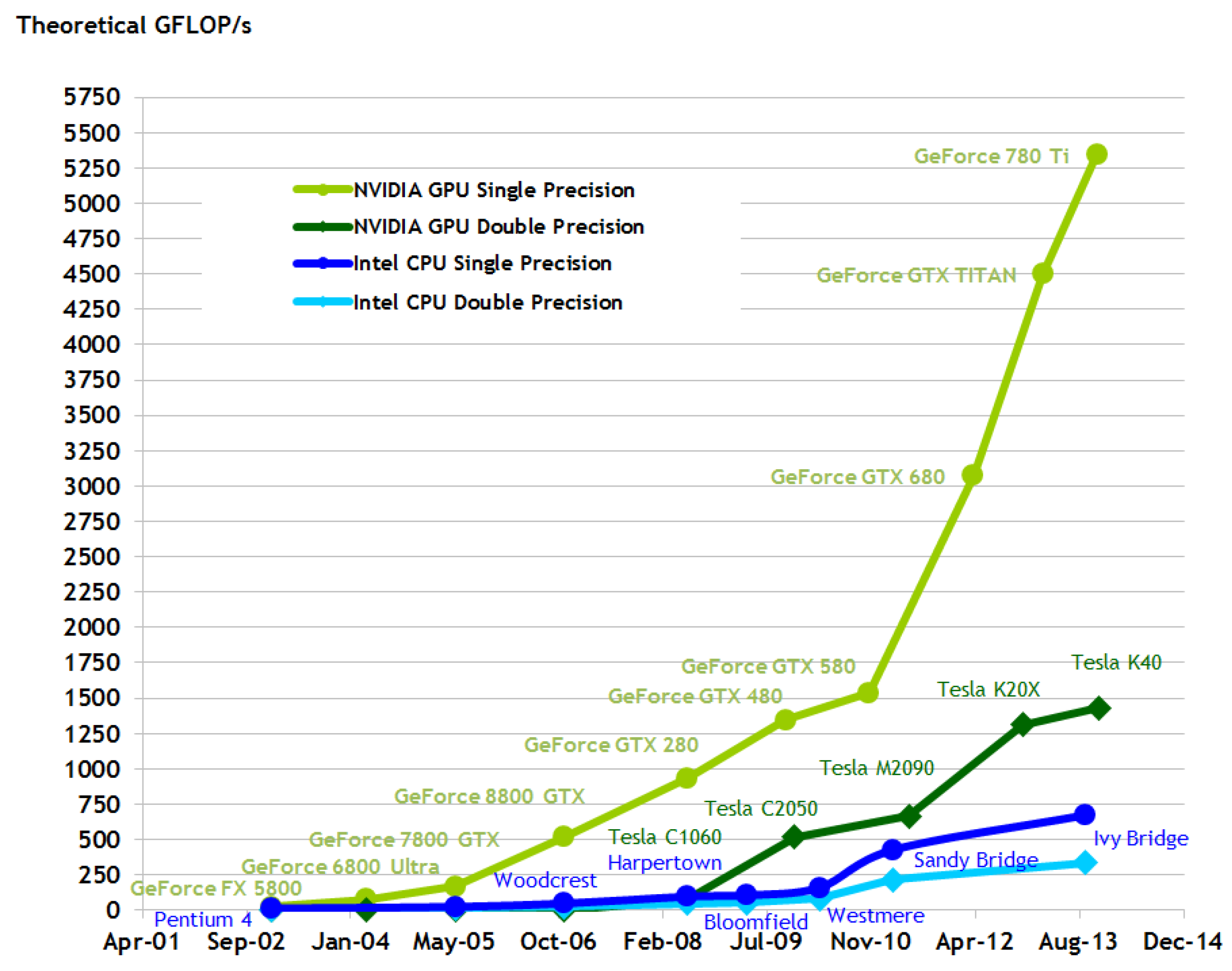
Figure 1 reports the evolution in GigaFLOPS (
i.e., billions of floating point operations per second in single and double precision) between GPUs and CPUs.
Despite the above-mentioned advances in GPUs, until 2006, only a few persons mastered the skills necessary to use GPUs to achieve better performance for only a limited number of applications. In 2007, NVIDIA released CUDA (Compute Unified Device Architecture, [
29]) programming language similar to the well known C/C++. This facilitated the transition to parallel programming on GPU. Nowadays the GPU programming languages have been improved (see [
30] for a review) and there is a software that use it to increase performances, see e.g., Mathematica, R and MATLAB.
MATLAB is a popular software in the economics and econometrics community (see, e.g., [
31]), which has introduced, starting with version R2010b, the support to GPU computing in its Parallel Computing Toolbox. This allows one to use raw CUDA code within a MATLAB program as well as already built-in functions that are directly executed on the GPU, see [
21] for a discussion about CUDA programming in econometrics.
With the massively parallel use of GPUs, researchers have achieved significant speedups in different applications, see [
21,
32,
33,
34,
35,
36] among others. However, as pointed out by [
21], such speed-ups are generally achieved only after extensive adaptation, optimization and tuning of the algorithms that is really time consuming. We comment on this point further in
Section 5. This brings forward two interesting challenges for parallelization: transforming traditional (sequential) algorithms to be suitable for a GPU implementation and achieving significant speed increase almost without any extra programming effort. In this paper, we describe our ParMitISEM algorithm and show that the provided algorithm can be used for a large set of models to gain speed increases without additional programming effort.
3. Parallel Implementation of MitISEM: ParMitISEM
ParMitISEM relies heavily on the use of IS in the MitISEM algorithm. IS ([
8,
9,
37,
38]) is a general method for estimating expectations of functions
of parameter
θ where the probability density function of
θ can be non-standard. Given a density kernel
for
θ, the method is based on draws from a candidate density
, instead of direct simulations from
. This indirect simulation method overcomes the issue of simulating from the non-standard density
. The candidate density
is chosen such that it is easy to simulate from and the draws from the candidate density are
weighted according to the IS weights. The necessary conditions for the candidate density and the finite sample properties of the estimator are discussed in [
38,
39].
Let Y denote the data, e.g., time series, and
θ denote the model parameters, where the posterior or
target density of parameters are denoted by
and simulating from this density is not trivial. In this case, the expected value of a function of parameters,
can be obtained using the following IS steps:
- (1)
Draw θ from a “similar and wide-enough” “importance/candidate density” , which should approximate reasonably well and should be straightforward to simulate from;
- (2)
Simulate M draws from ;
- (3)
Approximate the function of parameters
by:
where
for
are generated from
, and
.
Note that since
is a ratio, one can remove the constant of proportionality in this ratio and for
, the procedure provides estimated means of model parameters. The IS algorithm is based on weights
calculated from independent draws
. Due to this non-recursive structure, one can in principle assign each draw to each core and collect the results in (
1) at the end of the procedure.
We next illustrate how this parallelization strategy is implemented for ParMitISEM. As explained in [
7], the MitISEM consists of two parts. In the first part, a mixture of Student-
t candidate densities is fitted to the target using an EM algorithm where each step of the optimization procedure is weighted using IS. In the second stage, the obtained candidate density can be used in IS or the independence chain Metropolis–Hastings method for Bayesian inference on model parameters and model probabilities. Steps of the MitISEM algorithm are as follows:
- (1)
Initialization: Simulate draws from a “naive” candidate distribution with density , which is obtained as follows. First, we simulate candidate draws from a Student-t distribution with density , where the mode is taken equal to the mode of the target density and scale matrix equal to minus the inverse Hessian of the log-target density (evaluated at the mode), and where the degrees of freedom are chosen by the user. Second, the mode and scale of are updated using the IS-weighted EM algorithm. Note that is already a more advanced candidate than the commonly used ; typically yields a substantially worse numerical efficiency than .
- (2)
Adaptation: Estimate the target distribution”s mean and covariance matrix using IS with the draws from . Use these estimates as the mode and scale matrix of Student-t density . Draw a sample from this adaptive Student-t distribution with density , and compute the IS weights for this sample.
- (3)
Apply the IS-weighted EM algorithm given the latest IS weights and the drawn sample of step (1). The output consists of the new candidate density g with optimized set of parameters ζ. Draw a new sample from the distribution that corresponds with this proposal density and compute corresponding IS weights.
- (4)
Iterate on the number of mixture components: Given the current mixture of H components take of the sample that correspond to the highest IS weights. Construct with these draws and IS weights a new mode and scale matrix which are starting values for the additional component in the mixture candidate density. This choice ensures that the new component covers a region of the parameter space in which the previous candidate mixture had relatively too little probability mass. Given the latest IS weights and the drawn sample from the current mixture of H components, apply the IS-weighted EM algorithm to optimize the parameters of each mixture component. Draw a new sample from the mixture of components and compute corresponding IS weights.
- (5)
Assess convergence of the candidate density’s quality by inspecting the IS weights using the Coefficient of Variation of the IS weights (CoV) and return to step 4 unless the algorithm has converged.
As the algorithm shows, steps 2–5 in the algorithm rely on M IS draws and the calculation of the target and candidate density values. In these steps, each draw from the candidate density can be assigned to a different core that will carry out the necessary calculation independently, and the results will be collected at the end. For this reason, the parallelization strategy for ParMitISEM on CPUs and GPUs is straightforward. Note that the nature of the MitISEM algorithm in steps 2–5 is still sequential, despite the simplicity of parallelization of IS steps. Specifically, the iteration on the number of mixture components and iteration over the EM steps are the sequential parts of the algorithm, hence cannot be parallelized in a straightforward way. Still, these steps are computationally less demanding compared with obtaining IS draws and evaluating target and candidate densities and hence do not cause a large computational burden.
We note that especially step 3 of the algorithm, Expectation (E) and Maximization (M) steps of MitISEM, benefits from our parallelization strategy. We refer to [
7] for these steps where the
L-th E-step for the mixture of
H Student-
t densities is specified as follows:
where
,
is the digamma function (the derivative of the logarithm of the gamma function
),
is a
k-dimensional Student-
t density with mode
, scale
and degree of freedom
for
k model parameters, and
for
are the mixture weights of each Student-
t component. In this step, parameters
,
i.e., the candidate density’s parameters
, are obtained from the previous EM step
. Given the E-step, parameters are updated using the M-step:
where
are the importance weights of each draw
from the previous candidate
.
Further,
is solved from the first order condition of
:
In ParMitISEM, calculation of the expectations for each IS draw
i are done in parallel. In addition to this, summations in all parts of the M-step in (
6)–(
9) are also performed in parallel. This addition brings computational gains particularly for the optimization of (
9), where an approximate solution for the first order condition is obtained iteratively, but the value of the first order condition at each iteration of EM is obtained using parallel calculations for the summation terms.
We note that the parallelization we employ has the advantage of being a generally applicable method. Given any posterior or target density, ParMitISEM can be used to obtain an approximation and IS results using this approximation as a candidate. No alteration of the algorithm depending on the features of the posterior is required. In addition, implementations in GPU and CPU can be carried out in the same way since the parallelization strategy is also not specific to one of these implementations. Finally, ParMitISEM consists of a general IS procedure which is parallelized. This procedure can be used at the second stage, when the purpose is to use the ParMitISEM approximation as a candidate density for IS in Bayesian inference. In this case, speed gains from ParMitISEM are two-fold: First, ParMitISEM will reduce the computational time of obtaining the candidate density. Second, computational time required for the Bayesian inference using IS will improve using the IS procedure inherent in ParMitISEM.
4. Parallelization Experience for Four Econometric Models
In this section, we describe our experience with ParMitISEM for four canonical econometric models. The first case we consider is a non-elliptical bivariate density function, the Gelman–Meng density, presented in [
22]. The second case we consider is Bayesian inference of a GARCH(1,1) model with Student-
t errors, originally proposed by [
40], applied to daily S&P 500 log-returns. The third application we consider is Bayesian inference of the IV model applied to [
41] data on education and income, also analyzed in [
23]. The fourth and final model is Bayesian inference of the structural form of the New Keynesian Phillips Curve (NKPC) model capturing the relationship between marginal cost and inflation, applied to quarterly inflation and marginal costs in the US, also analyzed in [
42].
Due to the automatic and flexible nature of the MitISEM algorithm, all applications use a single parallel implementation of MitISEM, where only the target density has to be adjusted according to the application. Except for the Gelman–Meng density approximation, all applications make use of the ParMitISEM algorithm to obtain a candidate density for Bayesian inference of model parameters using a second IS step. We compare the CPU and GPU implementations of ParMitISEM in terms of the required computational time. The CPU and the GPU versions of the computer program are programmed in MATLAB. The CPU code uses all the available cores as well as the GPU counterpart.
2Our test machine is a regular desktop computer with a Core i7 4th generation (Corei7) with a total of eight cores. In the same machine, there is an NVIDIA Tesla 2075C (Tesla) that is a mid-range performance GPU, with 6GB memory and 448 cores. Moreover, we compare our results with an entry level NVIDIA GeForce 750M (GeForce) with a total of 384 CUDA cores and 2 GB of memory. MATLAB parallel toolbox license is required to run our code. All models are estimated using different number of IS draws within ParMitISEM: . In applications where the ParMitISEM approximation is used as a candidate for importance sampling for Bayesian inference, we also base the inference on M posterior draws.
4.1. Approximation of the Gelman–Meng Function
We consider the bivariate density described in [
22], for which the conditional distributions of variables
and
are normal distributions, while the joint distribution takes different non-elliptical forms depending on the parameter values:
where
is the vector of interest. Moreover, setting
in (
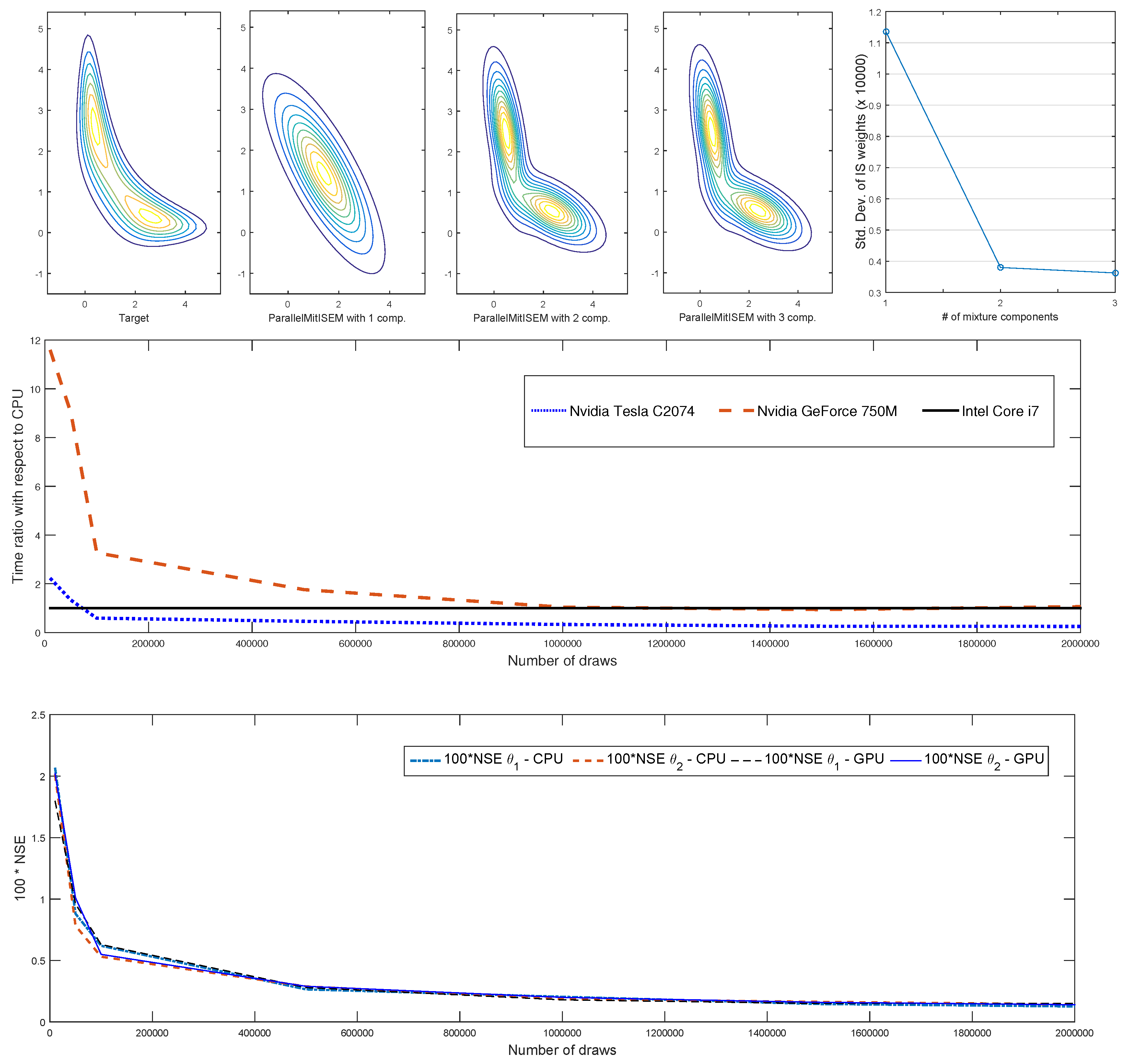
10) leads to a non-standard “banana shaped” contour presented in the upper left panel of
Figure 2. References [
7,
23] show that the standard MitISEM algorithm leads to substantial gains in approximating this density compared with the Gibbs sampler, MH and IS algorithms. We show that this computational gain can be improved using ParMitISEM.
We apply the ParMitISEM algorithm with different numbers of IS draws,
M, and, for each number of draws, we record the execution time and compare them between CPU and the GPU. Moreover, we calculate the Numerical Standard Error (NSE) for the CPU and GPU version of the program.
Figure 2 reports the results of this experiment. The top panel in
Figure 2 shows the target density kernel for the Gelman–Meng function with a “banana shaped” contour and the step-by-step approximations of this kernel using ParMitISEM. The target kernel has two clear modes and the ParMitISEM approximation stops with three mixture components. Even with this relatively low number of mixture components, the contour of the ParMitISEM approximation are similar to the contour of the target density. Gains from each additional component, presented in the top-right panel of
Figure 2, according to the CoV shows that the non-standard “banana shaped” contour of Gelman–Meng is well approximated with three mixture components, and the major improvement in this approximation is obtained by adding the second mixture component in ParMitISEM.
The middle panel in
Figure 2 presents the speed comparison between CPU and GPU implementations as the ratio of processing times in CPU and GPU, where a value below one indicates that the GPU computation is faster. Exact values of the computational time required for each implementation are reported in
Table 1. The table shows that the CPU implementation is superior to the Tesla GPU implementation for small number of draws, as soon as the number of draws increases, the GPU provides a clear improvement in computing time. This result is due to the parallel nature of the GPU with more available cores then the CPU. The other GPU (GeForce) performs relatively worse when the number of draws
M is small, and its performance improves as soon as the number of draws increases. Regarding the NSE, the CPU and GPU results are quite similar and the small numerical discrepancy between the NSE values disappear as soon as the number of draws increases.
4.2. Bayesian Inference of the GARCH(1,1) Model with Student-t Errors
The next canonical model we consider is the standard GARCH(1,1) model ([
40]) with Student-
t errors. The model is applied to daily percentage S&P 500 returns for the period between 2 January 1998 and 26 June 2015. Frequentist inference issues and the ill-behaved likelihood of GARCH type of models are reported in [
43]. Computational advantages of efficient and automatic sampling algorithms for the Bayesian inference of GARCH type of models are reported in [
5,
7,
23].
The
model with Student-
t errors for time series
is defined as follows:
where
is the conditional variance of
given the information set
and
denotes the Student-
t distribution with
degrees of freedom. In addition,
is treated as a known constant, set as the sample variance of the time series
, which will consist of daily stock index (log) returns in this example. We restrict
and
to ensure positivity of
,
to ensure a proper posterior density where posterior means and variances exist, and specify flat priors for the model parameters. Moreover, we truncate
ω and
μ such that these have proper (non-informative) priors. For the
dimensional parameter vector
, we have a uniform prior on
with
which implies covariance stationarity.
Bayesian inference of this model is time consuming and possibly inaccurate with a small number of draws for three reasons. First, the iterations required to obtain unobserved conditional variances in (
11) cannot be executed in parallel in a straightforward way. Second, the restrictions on model parameters imply that several IS draws, in a standard IS algorithm or in obtaining the MitISEM approximation, may be outside the relevant parameter space. Hence, a large number of draws are required to obtain a reasonable approximation to the candidate, or to obtain posterior draws of parameters unless an appropriate candidate density is used. Third, the posterior density is non-elliptical particularly due to the degree of freedom parameter. See [
5] among others for an extended discussion.
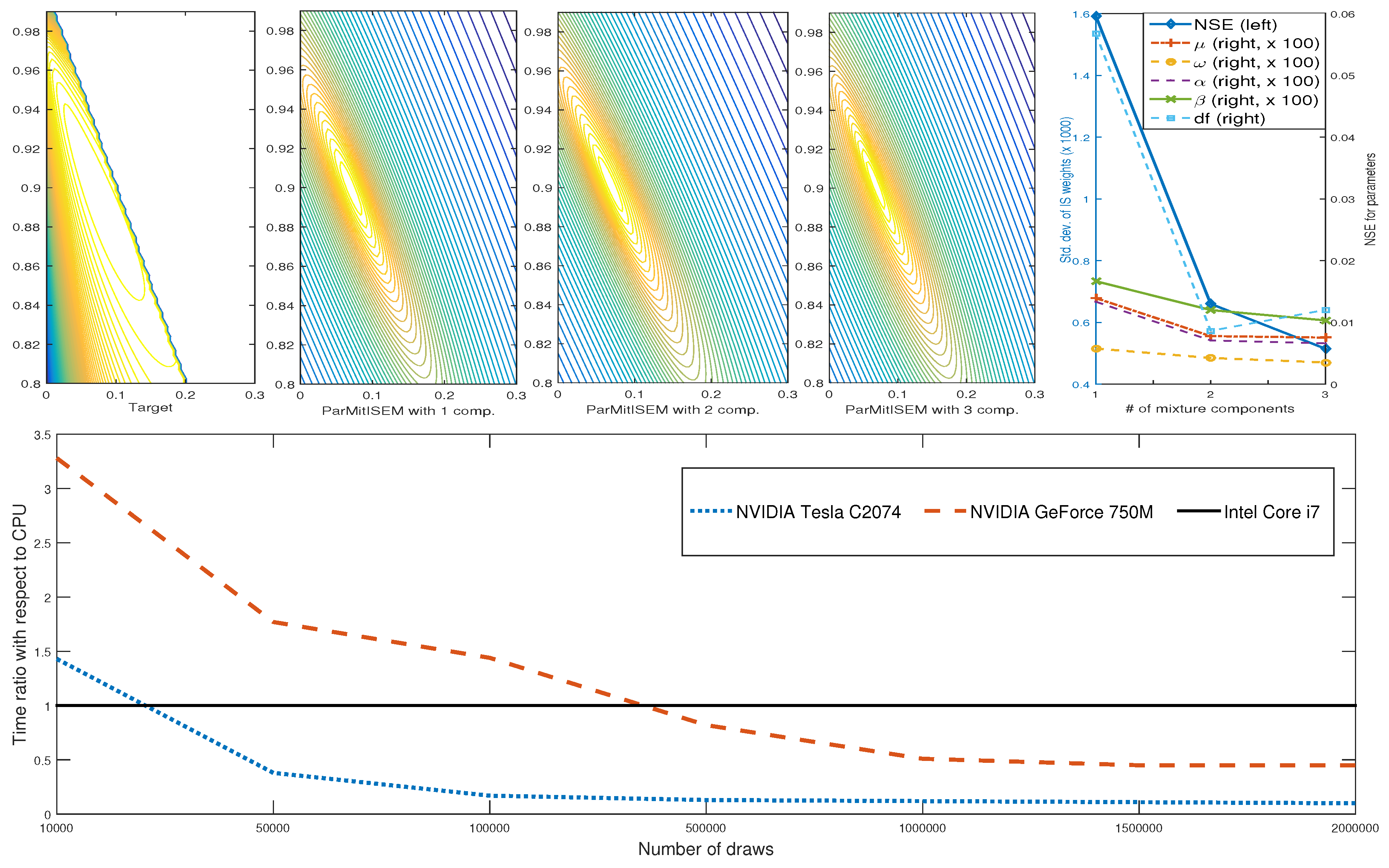
In order to perform Bayesian inference, we first obtain the ParMitISEM approximation to the joint posterior density of parameters. As a second step, the ParMitISEM candidate is used as the candidate density for the IS algorithm. The obtained ParMitISEM candidate in this example has three mixture components.
Figure 3 presents the joint posterior with respect to model parameters
where the remaining parameters are fixed at their posterior mean, together with the speed comparison of the CPU and GPU implementations of ParMitISEM to obtain the approximation to the joint posterior. Similar to the Gelman–Meng application, computational time is substantially improved with the GPU implementation. The top-right panel of
Figure 3 shows that the CoV values are improved with each additional mixture component. Similarly, the obtained NSE values for each parameter, except for the degree of freedom parameter, go down with additional mixture components. Particularly, the second mixture component improves the approximation accuracy substantially.
Table 2 reports the speed comparison between CPU and GPU as a GPU/CPU ratio. Similar to the Gelman–Meng distribution results, the CPU is superior to the Tesla GPU for small number of draws, but the Tesla GPU has a clear advantage for more reasonable (e.g., larger than 50,000) draws. In this application, even the GeForce that starts with a disadvantage becomes more competitive as soon as the number of draws increases.
Table 3 reports the IS estimator of
which is the posterior mean of the parameters based on the CPU and GPU implementations of ParMitISEM together with the difference in the posterior means between both implementations. For a relatively small number of draws, posterior means from the two implementations differ and this difference disappears when the number of draws increases.
An important point is the relatively large NSE for the degree of freedom parameter for draws. This NSE value indicates that the posterior density is highly non-standard especially with respect to the degree of freedom parameter. Therefore, a large number of draws are needed for an accurate inference of the model, and ParMitISEM is particularly useful in this application.
We finally note that functions of parameters, such as the sum of GARCH coefficients or the long-run variance of the GARCH model , are often of interest for GARCH models. Bayesian inference for such functions of parameters does not require an additional MitISEM approximation. Using the IS draws based on the MitISEM approximation, it is possible to calculate to infer these functions of parameters. In the example we provide, using the candidate obtained with 2,000,000 draws, we obtain the following results for these functions of parameters: Posterior mean for is 0.97 with an NSE value of , indicating a high persistence for the variance process, and an accurate estimation with a small NSE. In addition, the posterior for the unconditional variance is approximately 0.054 with an NSE value of .
4.3. Bayesian Inference of the Instrumental Variables Model
In this subsection, we present the application of ParMitISEM to an Instrumental Variables (IV) model. The model is applied to [
41] data on income and education. The IV model with one explanatory endogenous variable and
p instruments is defined by [
44]:
where the scalar
β and the
vector Π are model parameters,
y is the
vector of observations on the dependent variable income,
x is the
vector of observations on the endogenous explanatory variable, education,
z is the
matrix of observations on the instruments. All variables are demeaned,
i.e., both model equations do not include a constant term. The disturbances are assumed to come from a normal distribution:
, where
is a positive definite and symmetric
matrix,
I denotes the
identity matrix and ⊗ denotes the Kronecker product operator. The endogeneity problem of the variable
x arises from possible correlation between the disturbances, given as
for
.
The model in (
12)–(
13) is shown to have non-standard posterior densities unless the covariance matrix Σ is diagonal, see [
45,
46,
47,
48]. The properties of this model are also different from the GARCH(1,1) model in
Section 4.2. It is shown that the posterior density under a flat prior has a ridge at
, and it is not a proper density due to this ridge for
. This irregularity can be mitigated by the use of a Jeffrey’s prior see [
49]. In this case, the posterior is a proper density, but sampling methods such as the Gibbs sampler are not applicable, see [
6]. The applicability of the MitISEM algorithm to the IV model and the speed gains compared with the griddy-Gibbs sampler [
50] are shown in [
23]. In this section, we show that the ParMitISEM implementation provides substantial speed gains for the Bayesian inference of this model.
The [
41] data on income and education consist of the dependent variable equal to hourly wages in logarithms and the endogenous right hand side variable is given as educational level which takes the value of one if an individual attended college and zero otherwise. The instrument for the education level is “college proximity”, which takes the value of one if there is a nearby college and zero otherwise. Following [
23], we control for the remaining exogenous variables by regressing the income, education and college proximity data on exogenous covariates and applying the IV model to the residuals of these regressions.
Table 4 reports estimated parameters using ParMitISEM on the [
41] dataset on GPU and CPU. All applications of ParMitISEM lead to four mixture components in the approximation. As the table shows, the difference in CPU and GPU estimates is really small and dies out as soon as the number of draws increases. The estimated posterior means of the parameters are in line with [
49], and the difference between posterior means from CPU and GPU implementations of ParMitISEM are approximately zero only with a high number of draws from the posterior, implying that a large number of draws and a high computing time are required to obtain accurate estimates of these parameters.
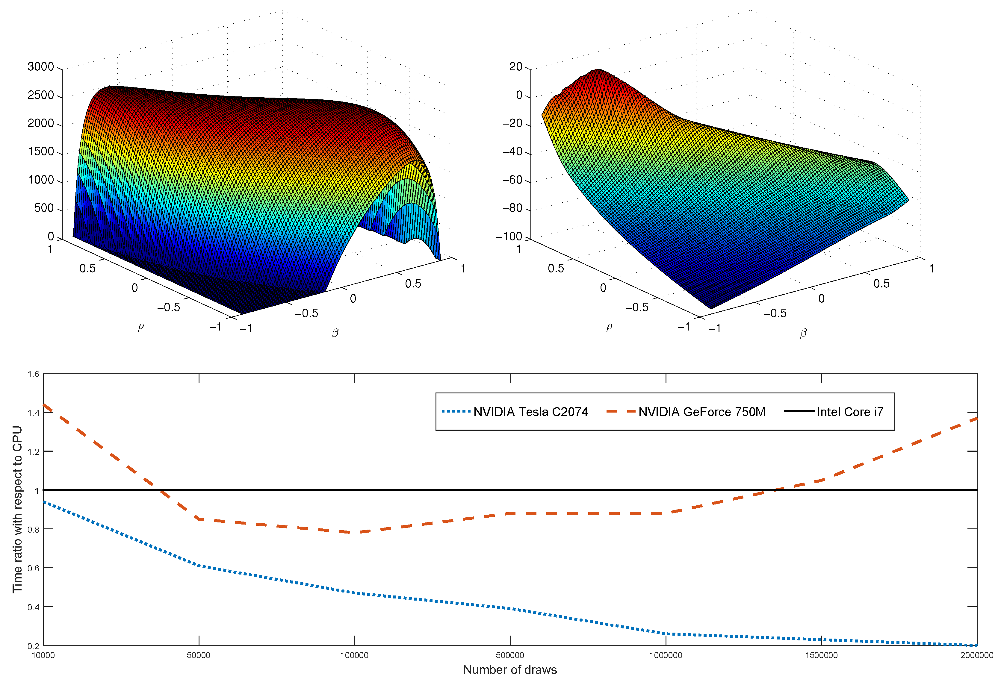
Table 5 and
Figure 4 present the speed comparison between CPU and GPU implementations of ParMitISEM, where a value below one indicates that the GPU implementation is faster compared with the CPU implementation. In this application, Tesla GPU is superior to the CPU for all considered number of draws. GeForce application, on the other hand, performs worse for small,
, and large,
and
number of draws. While a relatively poor performance of the GeForce application with a large number of draws is expected due to the saturation of the GPU,
i.e., the large number of draws causing a decrease in computing performance, yet this is not the case for the Tesla C2074.
An important feature in this application in terms of computational burden is the restriction in the parameter space
and the ridge of the posterior at
. These properties of the posterior leads to a large number of IS draws within ParMitISEM to have a zero posterior probability. We follow the robustness method provided in [
23] to improve the performance of the MitISEM method. Specifically, within the MitISEM algorithm, a rejection step is included to keep a subset of
M draws which lead to a non-zero posterior density. This robustification is applied in both CPU and GPU implementations of ParMitISEM and improves the approximation at the expense of a decreased number of effective number of draws
. An increase in
M does not automatically lead to a smaller NSE since several draws are “thrown away” with this robustification. We conjecture that this lack of comparability between NSE values for different
M explains the slightly higher NSE values for large
M shown in the bottom panel of
Table 5.
Restrictions in the parameter space also have a potential effect on the first step of the MitISEM algorithm. As discussed earlier, the initialization of the algorithm relies on the numerical evaluation of the Hessian matrix for the very first Student-t component. In models with tight parameter constraints, it is possible that this Hessian is not estimated properly or it is not estimated at all due to numerical accuracy. A straightforward method to avoid such a problem is to start the MitISEM algorithm with a user-defined Hessian, such as a diagonal matrix with positive diagonal entries. Such an initialization will possibly lead to an inefficient initial Student-t candidate which is very different from the target density. Despite this inefficiency, this initial Hessian is updated several times within the ParMitISEM procedure. Provided that the number of IS draws are large enough, the initial inefficiency of the Hessian is expected to have minimal effect on the final approximation.
4.4. Bayesian Inference of the Structural NKPC Model
In this subsection, we apply ParMitISEM to a highly non-linear econometric model, namely the structural form representation of the New Keynesian Philips Curve (NKPC) model for quarterly inflation and marginal costs in the US for the period between 1962Q2 and 2012Q4. We show that there are substantial gains from the ParMitISEM in this model in terms of the required computing time.
The structural form (SF) representation for the NKPC model is:
where
,
is quarterly inflation,
is quarterly marginal cost (demeaned and detrended) and the unobserved variable
can be derived as a function of the past marginal costs
and
. Standard stationary restrictions should hold for
and it is assumed that
.
As shown in [
42], solving for the unobserved inflation expectations on the right hand side of (
14) leads to the following model which is highly non-linear in structural parameters:
where the parameters
are again restricted according to the structural form NKPC model.
We specify flat priors for
, uninformative normal priors for
and inverse gamma priors for the residual variances, similar to [
42]. First, the ParMitISEM algorithm is used to approximate the joint posterior density of parameters. In a second step, this candidate density is used as a candidate density in IS to obtain posterior means and variances of the structural parameters.
Reference [
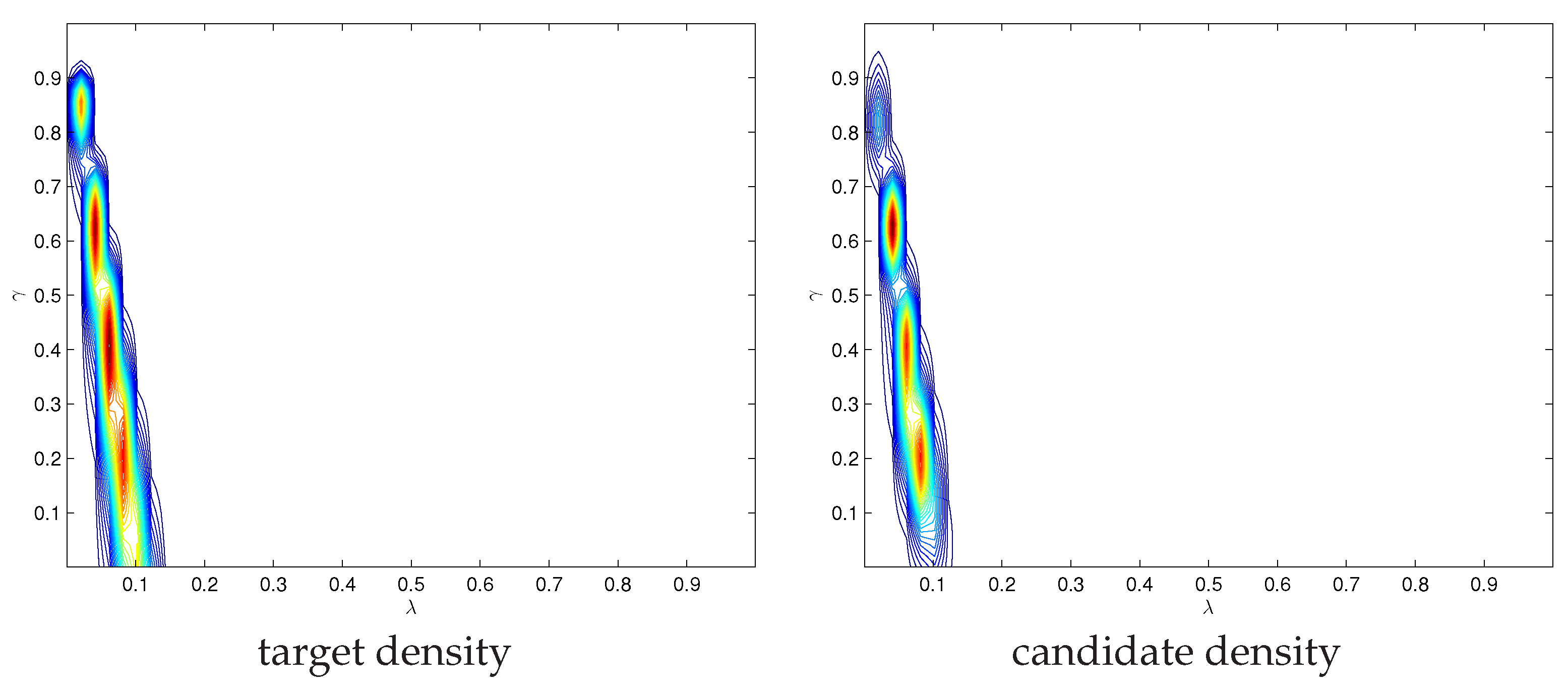
42] analyzes this model and extensions of it, and shows that the posterior densities of model parameters is highly non-standard due to the non-linear nature of the model and parameter restrictions. The shape of the posterior kernel, with respect to parameters
is shown in
Figure 5. The posterior density shown at the left panel of
Figure 5 has multiple modes, which are captured well by the MitISEM candidate on the right panel of
Figure 5. In addition,the posterior density has non-zero values only on a very restricted region for parameters
. This region is much smaller than the parameter space restricted through the priors,
. Hence, in this application, the use of MitISEM to obtain a candidate density resembling the posterior is important for improving MCMC methods’ convergence based on this candidate density. Despite this clear advantage, obtaining a good MitISEM candidate in this application is potentially time consuming due to the parameter restrictions and non-linearity in the model. Parameter estimates of the model and the computational speed comparisons for the CPU and GPU implementations of ParMitISEM are shown in
Table 6 and
Table 7, respectively, for different number of draws
M. We first note that obtaining a large number of draws, e.g., above 1,500,000 draws, using the CPU or GPU is not feasible in this model due to memory saturation arising from the large number of observations and draws, e.g., MATLAB gives the standard message “out of memory”, consequently more advanced clusters and GPU cards are required to obtain higher number of draws. For our purpose of speed comparison,
Table 6 and
Table 7 report results only for the number of draws which are possible to obtain in this model. Second, the same robustification step as in
Section 4.3 is used in ParMitISEM in order to remove draws which lead to zero posterior density values in the NKPC model. However, this robustness does not affect the general pattern in the obtained NSE values in CPU or GPU implementations: NSE values for all parameters reported on the bottom panel of
Table 7 typically go down with the number of draws
M. Posterior means of the structural parameters reported in
Table 6 are similar to those reported in [
42],
i.e., the candidate density obtained by ParMitISEM and the IS results are in line with the method used in [
42]. In this application, Tesla GPU is always superior to CPU in terms of computational time, regardless of the number of draws. Similar to the earlier experiments, the GeForce implementation only has an advantage for an increased number of draws, e.g., for
.
An important result is that the speed gains from Tesla and GeForce implementations in this applications are much higher than those obtained for the GARCH(1,1) model application in
Section 4.2. This result follows from our parallelization strategy and the properties of the GARCH(1,1) model posterior. The strategy we follow for parallelization is not tailored for each specific model.
i.e., we do not optimize the speed of the calculations of the GARCH model posterior and these calculations are done sequentially. With the parallelization of the general method, MitISEM, relative speed gains from the GPU are mainly determined by whether the posterior density has to be evaluated in a sequential manner. Additional gains from ParMitISEM can be achieved if the posterior density is adjusted to minimize the amount of sequential calculations.
5. Conclusions
This paper presents a parallelized version of MitISEM originally proposed by [
7] and refined in [
23]. MitISEM is a general and automatic algorithm based on IS for the approximation of a possibly non-elliptical target density using an adaptive mixture of Student-
t densities as approximating or candidate density. The parallelized version of MitISEM, ParMitISEM, is an implementation of this algorithm for GPU and multi-core CPU calculations.
The parallelization strategy is based on IS steps of the MitISEM algorithm, where we exploit the parallelization of the IS draws and functions of IS draws. It is shown with four examples that the implementation is not model specific, leading to a general algorithm which can be used to approximate a multi-dimensional target, e.g., a posterior density, without the need to parallelize the posterior density explicitly. We show that ParMitISEM is easy to implement in MATLAB and can run on GPUs and in multi-core CPUs. We present substantial speed gains from the GPU implementation of the ParMitISEM algorithm compared with the multi-core CPU implementation using four different models: The Gelman–Meng density, a GARCH(1,1) model with Student-t errors applied to S & P 500 daily returns, an IV model applied to data on income and education and a structural form NKPC model applied to quarterly US data. These applications have different properties in terms of the shape of the target density approximated by ParMitISEM. The speed gains from GPU implementation of ParMitISEM are particularly pronounced in case of highly irregular target densities where a large number of IS draws are required to obtain an accurate approximation to the target density.
Finally, a further comment regarding the speed gains of the GPU with respect to multicore CPU is in order. Some studies such as [
33,
51] document massive speed gains, from 35 up to 500, of the GPU code with respect to single-threaded CPU code. Considering these results, it can be concluded that our GPU speed performance could be increased substantially, this observation is right and wrong at the same time.
It is right because ParMitISEM could be written using just raw CUDA code. This low level programming language allows to get around memory bandwidth limitations and access directly to the internal GPU memory, such an implementation would increase tremendously the performance, as discussed in [
21]. These impressive speed gains occur at the cost of getting familiar with internal GPU architecture and CUDA programming language, knowledge that requires months to master.
The above statement is also wrong because the approach we propose is fast and easy to implement, and only a good familiarity of the MATLAB environment is required. No knowledge of the internal GPU architecture and the raw CUDA code are necessary. Of course, this approach cannot deliver the same performance of raw CUDA code, but this is the trade-off of easy implementation. Despite these limitations, the speed gains in our applications are considerable. In fact, to have roughly the same performance of the Tesla C2074 card on e.g., GARCH(1,1) model with 2,000,000 draws, the user will need a cluster with around 80 cores. Those clusters are expensive to buy and difficult to maintain; on the contrary, the Tesla C2074 fits in a normal desktop computer.
New versions of MATLAB continuously improve the performance of the GPU computing, and decreases the gap between raw CUDA code and MATLAB (GPU) code. Following these advances, improving the performance and the applicability of ParMitISEM without losing the ease of implementation is an interesting avenue of research.


