Comparing Markov Chain Samplers for Molecular Simulation

Abstract

Markov chain Monte Carlo sampling propagators, including numerical integrators for stochastic dynamics, are central to the calculation of thermodynamic quantities and determination of structure for molecular systems. Efficiency is paramount, and to a great extent, this is determined by the integrated autocorrelation time (IAcT). This quantity varies depending on the observable that is being estimated. It is suggested that it is the maximum of the IAcT over all observables that is the relevant metric. Reviewed here is a method for estimating this quantity. For reversible propagators (which are those that satisfy detailed balance), the maximum IAcT is determined by the spectral gap in the forward transfer operator, but for irreversible propagators, the maximum IAcT can be far less than or greater than what might be inferred from the spectral gap. This is consistent with recent theoretical results (not to mention past practical experience) suggesting that irreversible propagators generally perform better if not much better than reversible ones. Typical irreversible propagators have a parameter controlling the mix of ballistic and diffusive movement. To gain insight into the effect of the damping parameter for Langevin dynamics, its optimal value is obtained here for a multidimensional quadratic potential energy function.

1. Summary

Thermodynamic and structural properties of a molecular system can be precisely defined as ensemble-dependent expectations of functions of its configuration. The calculation of such expectations is feasible only with the use of Markov chain Monte Carlo (MCMC) methods or approximations thereof. Considered here are sampling propagators that do not compromise the Markov property. Included are unbiased samplers that conditionally accept proposed moves and biased samplers that unconditionally accept such moves, in particular, discretized stochastic dynamics. Many such sampling propagators are proposed in the literature, and, in virtually all cases, experiments are conducted to substantiate claims of superiority. Too often though, a good metric is not used to measure the computational cost of a propagator. The aim of this article is threefold: first, to explore some practicalities related to measuring the efficiency of a propagator; second, to highlight the superior efficiency of irreversible propagators, namely, those that do not satisfy detailed balance; and third, to provide some insight into the optimal mix of diffusive and ballistic movement for Langevin dynamics.

Let ${\rho }_{\mathbf{Q}}\left(\mathbf{q}\right)$, $\mathbf{q}={[q_1,q_2,\dots ,q_{\nu }]}^{\mathsf{T}}$ denote the probability density function corresponding to the ensemble of interest. This function is assumed to be known only up to a multiplicative factor. An observable is an expectation $\mathbb{E}\left[u\left(\mathbf{Q}\right)\right]=\int u\left(\mathbf{q}\right){\rho }_{\mathbf{Q}}\left(\mathbf{q}\right)\mathrm{d}\mathbf{q}$ for some “preobservable” $u\left(\mathbf{q}\right)$. This can be estimated by the mean ${\overline{U}}_N=(1/N){\sum }_{n=0}^{N-1}u\left({\mathbf{Q}}_n\right)$, where the random values ${\mathbf{Q}}_n$ are obtained from a Markov chain ${\mathbf{Q}}_0\to {\mathbf{Q}}_1\to \cdots \to {\mathbf{Q}}_{N-1}$ that samples from ${\rho }_{\mathbf{Q}}\left(\mathbf{q}\right)$. Note the use here of upper case to denote random variables.

In practice, sampling performance is improved if the configuration variables $\mathbf{q}$ are augmented with auxiliary variables $\mathbf{p}$, e.g., momenta, yielding phase space variables $\mathbf{z}=(\mathbf{q},\mathbf{p})$. The probablity density is extended to $\rho (\mathbf{q},\mathbf{p})$ so that

$$\int \rho (\mathbf{q},\mathbf{p})\mathrm{d}\mathbf{p}={\rho }_{\mathbf{Q}}\left(\mathbf{q}\right),$$

and an MCMC scheme is constructed to produce a chain ${\mathbf{Z}}_0\to {\mathbf{Z}}_1\to \cdots \to {\mathbf{Z}}_{N-1}$, where $\mathbf{Z}=(\mathbf{Q},\mathbf{P})$.

The samples from the chain tend to be highly correlated, and this greatly reduces the convergence rate as $N\to +\infty$. As explained in Section 2, the variance of an estimate for $\mathbb{E}\left[u\right(\mathbf{Z}\left)\right]$ is

$$\mathrm{Var}\left[{\overline{U}}_N\right]=\frac{\tau }{N}\mathrm{Var}\left[u\left(\mathbf{Z}\right)\right]+\mathcal{O}(\frac{1}{N^2})$$

(1)

where $\tau$ is the integrated autocorrelation time (IAcT) for $u\left(\mathbf{z}\right)$. The effective sample size is therefore $N/\tau$, and the appropriate metric for evaluating a propagator is the effective sample size divided by the computing time.

In a great many practical simulations, the effective sample size is probably close to zero. One can disagree on the significance of such simulations [1]. In any case, for the comparison of sampling algorithms, it is possible to choose molecular systems, restrained if necessary, for which it is feasible to attain a decent effective sample size.

Often, the spectral gap is cited as the relevant quantity. To understand its role, it is helpful to express ideas in a direct way as in Refs. [2,3]. As detailed in Section 2, introduce a forward transfer operator $\mathcal{F}$ to express the ratio ${\rho }_n/\rho$ in terms of ${\rho }_{n-1}/\rho$, where ${\rho }_n\left(\mathbf{z}\right)$ is the probablity density for ${\mathbf{Z}}_n$. Let ${\mathcal{F}}_0=\mathcal{F}-\mathcal{E}$ where $\mathcal{E}u$ denote the function with constant value $\mathbb{E}\left[u\right(\mathbf{Z}\left)\right]$. Assume that the operator ${\mathcal{F}}_0$ has its spectrum strictly inside the unit circle, as it does in practice. The error in $(1/N){\sum }_{n=0}^{N-1}{\rho }_n\left(\mathbf{z}\right)$ can be shown [1] to be “proportional to” ${(1-{\mathcal{F}}_0)}^{-1}$ and therefore to the reciprocal of the spectral gap $|1-{\lambda }_2|$, where ${\lambda }_2$ is a nonunit eigenvalue of $\mathcal{F}$ nearest 1.

Estimates of the IAcT are obtained by summing the terms of the autocorrelation function, which is constructed from autocovariances of increasing time lags normalized by the (lag zero) covariance. Each term contributes a roughly equal statistical error but a signal that decays as the lag time increases. Therefore, in practice, the terms are weighted by a function called a lag window. The lag window must be tailored to the autocorrelation function, and choosing a suitable lag window is very difficult, as mentioned in Section 2.1.

Reliable estimates of the IAcT are impractical in general. Section 3 reviews the concept of quasi-reliability, which aims to enforce a necessary condition for reliable estimates. Informally, the goal is to ensure good coverage of those “parts” of phase space that has been explored, to reduce the possibility of missing an opening to an unexplored part of phase space. More precisely, for an arbitrary subset of phase space, we ask that the proportion of samples in that subset differ from its expectation by no more than some tolerance $\mathit{tol}$, with, say, 95% confidence. This is shown to be true if the IAcT $\tau$ for any preobservable $u\left(\mathbf{z}\right)$ satisfies $\tau \le {\mathit{tol}}^{2}N$. The maximum IAcT ${\tau }_{max}$ is the greatest eigenvalue of

$$\mathcal{G}=1-\mathcal{E}+{\mathcal{F}}_0{(1-{\mathcal{F}}_0)}^{-1}+{\mathcal{F}}_0^{†}{(1-{\mathcal{F}}_0^{†})}^{-1},$$

(2)

where ${}^{†}$ denotes the adjoint with respect to the inner product

$$\langle v,u\rangle =\int \overline{v\left(\mathbf{z}\right)}u\left(\mathbf{z}\right)\rho \left(\mathbf{z}\right)\mathrm{d}\mathbf{z}.$$

For a reversible propagator, where ${\mathcal{F}}^{†}=\mathcal{F}$, ${\tau }_{max}$ is 1 less than twice the reciprocal of the spectral gap. However, for an irreversible propagator, it can be much smaller, as demonstrated by a simple example in Section 4.1, or larger as in Section 5. As a practical algorithm, it is suggested to estimate the maximum IAcT by discretizing the space of preobservables. Consideration of a quadratic energy potential suggests using a linear combination of phase space variables (and possibly quadratic terms in these variables).

The idea of seeking the preobservable that maximizes the IAcT is suggested already in Ref. [4], which considers a set of indicator functions as preobservables and uses the greatest IAcT of these to assess sampling thoroughness. In general, maximizing over a linear combination of preobservables can lead to a much larger result than taking the maximum of them individually, due to correlations that might exist between different preobservables. This does not necessarily apply, however, to those considered in Refs. [1,4].

Section 3.1 notes that that typical irreversible propagators, termed “quasi-reversible” here, have a forward transfer operator $\mathcal{F}=\mathcal{R}\overline{\mathcal{F}}$, where each of $\overline{\mathcal{F}}$ and $\mathcal{R}$ is reversible and ${\mathcal{R}}^2=1$. For such propagators, the estimation of ${\tau }_{max}$ simplifies somewhat.

Theoretical results [5] indicate that adding irreversibility reduces the autocorrelation times of observables. Section 4 gives a couple of very elementary examples illustrating the dramatic increase in ${\tau }_{max}$ if an irreversible propagator $\mathcal{F}$ is replaced by its reversible “counterpart” $\frac{1}{2}(\mathcal{F}+{\mathcal{F}}^{†})$.

Discretized Langevin dynamics is a particularly effective general-purpose propagator. Unfortunately, one must specify a value for the damping coefficient $\gamma$. Section 5 analyzes ${\tau }_{max}$ for a quadratic potential and obtains an optimal value for the coefficient, namely, the value ${(3/8)}^{1/2}=0.612\cdots$ times the critical damping coefficient for lowest frequency ${\omega }_1$. This value is such that the lowest frequency mode is moderately underdamped, with higher frequencies increasingly underdamped.

2. Preliminaries

Assuming that ${\mathbf{Z}}_0$ has probability density $\rho \left(\mathbf{z}\right)$, the variance of the estimate ${\overline{U}}_N$ is exactly

$$\mathrm{Var}\left[{\overline{U}}_N\right]=\frac{1}{N}\mathrm{Var}\left[u\left(\mathbf{Z}\right)\right]\left(1+2\sum _{k=1}^{N-1}\left(1-\frac{k}{N}\right)\frac{C\left(k\right)}{C\left(0\right)}\right)$$

where the autocovariances

$$C\left(k\right)=\mathbb{E}\left[\left(u\left({\mathbf{Z}}_0\right)-\mathbb{E}\left[u\left({\mathbf{Z}}_0\right)\right]\right)\left(u\left({\mathbf{Z}}_k\right)-\mathbb{E}\left[u\left({\mathbf{Z}}_k\right)\right]\right)\right].$$

The limit $N\to +\infty$ gives Equation (1) where the integrated autocorrelation time

$$\tau =1+2\sum _{k=1}^{+\infty }\frac{C\left(k\right)}{C\left(0\right)}.$$

(3)

As an example of augmenting configuration space, consider $\rho (\mathbf{q},\mathbf{p})\propto exp(-\beta \left(V\left(\mathbf{q}\right)\right)+\frac{1}{2}{\mathbf{p}}^{\mathsf{T}}{M}^{-1}\mathbf{p}))$, where $\mathbf{p}={[p_1,p_2,\dots ,p_{\nu }]}^{\mathsf{T}}$. A good propagator for this is the BAOAB integrator [6] for Langevin dynamics, whose equations are

$$\mathrm{d}{\mathbf{Q}}_t=M^{-1}{\mathbf{P}}_t\mathrm{d}t,\mathrm{d}{\mathbf{P}}_t=\mathbf{F}\left({\mathbf{Q}}_t\right)\mathrm{d}t-\gamma {\mathbf{P}}_t\mathrm{d}t+\sqrt{\frac{2\gamma }{\beta }}{M}_{1/2}\mathrm{d}{\mathbf{W}}_t,$$

(4)

where M is a matrix chosen to compress the range of vibrational frequencies, $\mathbf{F}\left(\mathbf{q}\right)=-\nabla V\left(\mathbf{q}\right)$, $M_{1/2}{M}_{1/2}^{\mathsf{T}}=M$, and ${\mathbf{W}}_t$ is a vector of independent standard Wiener processes. Each step of the integrator consists of the following substeps:

• B: ${\mathbf{P}}_n^{\prime }={\mathbf{P}}_{n-1}+\frac{1}{2}\mathsf{\Delta }t\mathbf{F}\left({\mathbf{Q}}_{n-1}\right)$,
• A: ${\mathbf{Q}}_n^{\prime }={\mathbf{Q}}_{n-1}+\frac{1}{2}\mathsf{\Delta }t{M}^{-1}{\mathbf{P}}_n^{\prime }$,
• O: ${\mathbf{P}}_n^{″}=exp(-\gamma \mathsf{\Delta }t){\mathbf{P}}_n^{\prime }+\sqrt{1-exp(-2\gamma \mathsf{\Delta }t)}{\beta }^{-1/2}{M}_{1/2}{\mathbf{R}}_n$,
• A: ${\mathbf{Q}}_n={\mathbf{Q}}_n^{\prime }+\frac{1}{2}\mathsf{\Delta }t{M}^{-1}{\mathbf{P}}_n^{″}$,
• B: ${\mathbf{P}}_n={\mathbf{P}}_n^{″}+\frac{1}{2}\mathsf{\Delta }t\mathbf{F}\left({\mathbf{Q}}_n\right)$,

where ${\mathbf{R}}_n$ is a vector of independent standard Gaussian random variables. The samples generated from this process are shown [7] to be those from a distribution that differs from the correct one by only $\mathcal{O}\left(\mathsf{\Delta }{t}^2\right)$. The special choice $\gamma =1/\left(2\mathsf{\Delta }t\right)$ is the Euler–Leimkuhler–Matthews integrator [6] for Brownian dynamics with step size $\delta t=\mathsf{\Delta }{t}^2/2$. Remarkably, the invariant density of this integrator differs from the correct one by only $\mathcal{O}\left(\delta t^2\right)$. This integrator can be expressed as a Markov chain ${\mathbf{Q}}_1^{\prime }\to {\mathbf{Q}}_2^{\prime }\to \cdots \to {\mathbf{Q}}_{N-1}^{\prime }$ in configuration space, with propagator

• ${\mathbf{Q}}_n={\mathbf{Q}}_n^{\prime }+\frac{1}{2}\sqrt{2\delta t}{\beta }^{-1/2}{M}_{1/2}^{-\mathsf{T}}{\mathbf{R}}_n$,
• ${\mathbf{Q}}_{n+1}^{\prime }={\mathbf{Q}}_n+\delta t{M}^{-1}\mathbf{F}\left({\mathbf{Q}}_n\right)+\frac{1}{2}\sqrt{2\delta t}{\beta }^{-1/2}{M}_{1/2}^{-\mathsf{T}}{\mathbf{R}}_n$,

which is a discretization of Brownian dynamics

$$\mathrm{d}{\mathbf{Q}}_t=M^{-1}\mathbf{F}\left({\mathbf{Q}}_t\right)\mathrm{d}t+\sqrt{\frac{2}{\beta }}{M}_{1/2}^{-\mathsf{T}}\mathrm{d}{\mathbf{W}}_t.$$

(5)

The desired samples $\left\{{\mathbf{Q}}_n\right\}$ are available as part of the process (and, as a theoretical observation, they can be recovered from the Markov chain $\left\{{\mathbf{Q}}_n^{\prime }\right\}$ alone, by eliminating ${\mathbf{R}}_n$ in the two equations above and solving for ${\mathbf{Q}}_n$).

For any MCMC propagator, the forward transfer operator is defined so that

$$u_n=\mathcal{F}{u}_{n-1}$$

where $u_n\left(\mathbf{z}\right)={\rho }_n\left(\mathbf{z}\right)/\rho \left(\mathbf{z}\right)$ and ${\rho }_n\left(\mathbf{z}\right)$ is the probability density for ${\mathbf{Z}}_n$. In particular,

$$\mathcal{F}{u}_{n-1}\left(\mathbf{z}\right)=\frac{1}{\rho \left(\mathbf{z}\right)}\int \rho \left(\mathbf{z}\right|{\mathbf{z}}^{\prime })u_{n-1}\left({\mathbf{z}}^{\prime }\right)\rho \left({\mathbf{z}}^{\prime }\right)\mathrm{d}{\mathbf{z}}^{\prime }$$

where $\rho \left(\mathbf{z}\right|{\mathbf{z}}^{\prime })$ is the transition probablity for the chain. The operator $\mathcal{F}$ has an eigenfunction ${\phi }_1\left(\mathbf{z}\right)\equiv 1$ for eigenvalue ${\lambda }_1=1$.

A reversible propagator is one that satisfies detailed balance, which means that

$$\rho \left({\mathbf{z}}^{\prime }\right|\mathbf{z})\rho \left(\mathbf{z}\right)=\rho \left(\mathbf{z}\right|{\mathbf{z}}^{\prime })\rho \left({\mathbf{z}}^{\prime }\right).$$

Detailed balance is equivalent to ${\mathcal{F}}^{†}=\mathcal{F}$, where the adjoint ${\mathcal{F}}^{†}$ is defined by the condition that $\langle \mathcal{F}v,u\rangle =\langle v,{\mathcal{F}}^{†}u\rangle$ for arbitrary $u\left(\mathbf{z}\right)$ and $v\left(\mathbf{z}\right)$. The BAOAB integrator is not reversible as a sampling propagator, except for the special case $\gamma =1/\left(2\mathsf{\Delta }t\right)$; however, a scheme consisting of a fixed number of BAOAB steps followed by a momenta flip is reversible. The unmodified BAOAB integrator is, however, in a class of “quasi-reversible” integrators introduced in Section 3.1.

As a model problem for Brownian dynamics, given by Equation (5), consider $F\left(q\right)=-m{\omega }^{2}q$. (The absence of boldface indicates scalar quantities.) Changing variables $Q_t={\left(m\beta \right)}^{-1/2}{Q}_t^{\prime }$ and dropping the prime gives the simple stochastic differential equation

$$\mathrm{d}{Q}_t=-{\omega }^2{Q}_t\mathrm{d}t+\sqrt{2}\mathrm{d}{W}_t,$$

(6)

where $W\left(t\right)$ denotes a standard Wiener process. A perfect realization of $Q\left(t\right)$ at discrete points is obtained by the reversible propagator

$$Q_n=exp(-{\omega }^2\delta t)Q_{n-1}+\sqrt{1-exp(-2{\omega }^2\delta t)}\frac{1}{\omega }{R}_n.$$

(7)

The probablity density $\rho (q,t)$ for $Q\left(t\right)$ satisfies the Fokker–Planck equation $(\partial /\partial t)\rho =(\partial /\partial q)\left({\omega }^{2}q\rho \right)+({\partial }^2/\partial q^2)\rho$. Writing $\rho (q,t)=u(q,t)\rho \left(q\right)$ gives $(\partial /\partial t)u=-{\omega }^{2}q(\partial /\partial q)u+({\partial }^2/\partial q^2)u$. The operator on the right-hand side has eigenfunctions $u\left(q\right)={\mathit{He}}_k\left(\omega q\right)$ with eigenvalues $-k{\omega }^2$ for $k=0,1,\dots$. The modified version of the Hermite polynomial of degree k is given by ${\mathit{He}}_k\left(x\right)={(-1)}^{k}exp(x^2/2)({\mathrm{d}}^n/\mathrm{d}{x}^n)exp(-x^2/2)$. The forward transfer operator $\mathcal{F}$ for the propagator defined by Equation (7) has these same eigenfunctions and has eigenvalues ${\lambda }_{k+1}=exp(-k{\omega }^2\delta t)$ for $k=1,2,\dots$. The spectral gap is $1-exp(-{\omega }^2\delta t)$. In the multidimensional case with normal mode frequencies $0<{\omega }_1\le {\omega }_2\le \cdots \le {\omega }_{\nu }$, the time step $\delta t$ is some fraction, say $\frac{1}{2}$, of $1/{\omega }_{\nu }^2$ and the spectral gap is very nearly $\frac{1}{2}{\omega }_1^2/{\omega }_{\nu }^2$. To see the applicability to practical numerical integrators, consider the Euler–Leimkuhler–Matthews discretization of Equation (6):

$$Q_n^{\prime }=(1-{\omega }^2\delta t)Q_{n-1}^{\prime }+(1-\frac{1}{2}{\omega }^2\delta t)\sqrt{2{\omega }^2\delta t}\frac{1}{\omega }{R}_n.$$

(8)

Comparing Equations (8) and (7) and equating the coefficients of the two terms on their right-hand sides enables Equation (8) to be written in the form of Equation (7) with modified values for $\omega$ and $\delta t$. In particular, the modified value of $exp(-{\omega }^2\delta t)$ is $1-{\omega }^2\delta t$, so spectral gap is exactly ${\omega }^2\delta t$. In the multidimensional case, where ${\omega }_1^2\delta t\ll 1$, the spectral gap for the discrete stochastics is very nearly that of the continuous stochastics.

2.1. Estimating Integrated Autocorrelation Time

Suggested [8] as a covariance estimate is the quantity

$$C_N\left(k\right)=\frac{1}{N}\sum _{n=0}^{N-k-1}(u\left({\mathbf{z}}_n\right)-{\overline{U}}_N)(u\left({\mathbf{z}}_{n+k}\right)-{\overline{U}}_N),$$

with justification in Ref. [9] (pp. 323–324).

The use of all possible terms $C_N\left(k\right)/C_N\left(0\right)$ in Equation (3) to estimate the IAcT does not converge in the limit $N\to +\infty$, so, in practice, a lag window $w\left(k\right)$ is used to increasingly damp terms as the noise to signal ratio increases:

$$\tau \approx 1+\sum _{k=1}^{N-1}w\left(k\right)\frac{C_N\left(k\right)}{C_N\left(0\right)}.$$

An interesting algorithm called acor for estimating the IAcT is available on the web [10]. Estimating the IAcT can be quite difficult, and acor can give unsatisfactory results. An attempt to improve it [1] is at best marginally successful. For reversible methods, there are properties of the autocorrelation function that may be useful for improving estimates of it [8].

3. Quasi-Reliable Estimates of Sampling Thoroughness

The idea of quasi-reliability is to require that the sample size N be large enough that, with say 95% confidence, the estimated probability of any subset $\Omega$ of phase space differs by no more than $\mathit{tol}$ from its correct value. More specifically, for any subset $\Omega$ of phase space, an estimate ${\overline{1_{\Omega }}}_{,N}$ of $\mathbb{E}\left[1_{\Omega }\left(\mathbf{Z}\right)\right]=Pr(\mathbf{Z}\in \Omega )$ must satisfy

$$\mathrm{Var}\left[{\overline{1_{\Omega }}}_{,N}\right]\le \frac{1}{4}{\mathit{tol}}^2.$$

Because

$$\mathrm{Var}\left[{\overline{1_{\Omega }}}_{,N}\right]\approx {\tau }_{\Omega }\frac{1}{N}\mathrm{Var}\left[1_{\Omega }\left(\mathbf{Z}\right)\right]\le \frac{1}{4N}{\tau }_{\Omega },$$

where ${\tau }_{\Omega }$ is the IAcT for $1_{\Omega }$, it is enough that

$$\frac{1}{4N}{\tau }_{\Omega }\le \frac{1}{4}{\mathit{tol}}^2\text{for all }\Omega .$$

(9)

For molecular simulations, this requires that only those conformations or clusters of conformations having a probability greater than $\mathit{tol}$ be sampled.

In practice, molecular systems have many symmetries, which dramatically reduces the amount of sampling needed. For example, water molecules are generally considered interchangeable as are many subsets of atoms on a given molecule, e.g., the 2 hydrogen atoms of any water molecule. More formally, there are permutations P of the variables $\mathbf{z}$ such that $\rho \left(P\mathbf{z}\right)=\rho \left(\mathbf{z}\right)$ and that ${\mathcal{P}}^{-1}\mathcal{F}\mathcal{P}=\mathcal{F}$ where $\left(\mathcal{P}u\right)\left(\mathbf{z}\right)=u\left(P\mathbf{z}\right)$. For such symmetries P, the quasi-reliablity requirement considers only those $\Omega$ for which $1_{\Omega }\left(P\mathbf{z}\right)=1_{\Omega }\left(\mathbf{z}\right)$.

It is helpful to express the IAcT in terms of the forward transfer operator. It can be shown that

$$\mathbb{E}\left[v\left({\mathbf{Z}}_0\right)u\left({\mathbf{Z}}_k\right)\right]=\langle {\mathcal{F}}^{k}v,u\rangle .$$

and, in particular,

$$\begin{array}{ccc}\hfill C\left(k\right)& =& \mathbb{E}\left[u\left({\mathbf{Q}}_0\right)u\left({\mathbf{Q}}_k\right)\right]-\mathbb{E}\left[u\left({\mathbf{Q}}_0\right)\right]\mathbb{E}\left[u\left({\mathbf{Q}}_k\right)\right]=\langle {\mathcal{F}}^{k}u,u\rangle -\langle \mathcal{E}u,u\rangle \hfill \\ \hfill & =& \left\{\begin{array}{cc}\langle (1-\mathcal{E})u,u\rangle ,\hfill & \text{for }k=0,\hfill \\ \langle {\mathcal{F}}_0^{k}u,u\rangle ,\hfill & \text{for }k\ge 1,\hfill \end{array}\right.\hfill \end{array}$$

(10)

using the fact that $\mathcal{E}{\mathcal{F}}_0={\mathcal{F}}_0\mathcal{E}=0$. The integrated autocorrelation time can be rewritten as

$$\tau =\frac{C\left(0\right)+2{\sum }_{k=1}^{+\infty }C\left(k\right)}{C\left(0\right)}=\frac{\langle (1-\mathcal{E}+2{\sum }_{k=1}^{+\infty }{\mathcal{F}}_0^k)u,u\rangle }{\langle (1-\mathcal{E})u,u\rangle }=\frac{\langle \mathcal{G}u,u\rangle }{\langle (1-\mathcal{E})u,u\rangle }$$

where

$$\mathcal{G}=1-\mathcal{E}+{\mathcal{F}}_0{(1-{\mathcal{F}}_0)}^{-1}+{({\mathcal{F}}_0{(1-{\mathcal{F}}_0)}^{-1})}^{†},$$

which is a self-adjoint operator.

For a reversible propagator, for which $\mathcal{F}$ and hence ${\mathcal{F}}_0$ is self adjoint, an arbitrary preobservable u is in many cases expressible as a linear combination of the eigenfunctions ${\phi }_k\left(\mathbf{z}\right)$ of ${\mathcal{F}}_0$, corresponding to eigenvalues $1>{\lambda }_2\ge {\lambda }_3\ge \cdots >-1$. (For a more rigorous treatment, see Ref. [8] (Section 2).) The IAcT for u is then simply a weighted average, of the values

$$1+\frac{2{\lambda }_k}{1-{\lambda }_k}=\frac{1+{\lambda }_k}{1-{\lambda }_k}$$

with weights ${\langle {\phi }_k,u\rangle }^2/\left(\langle {\phi }_k,{\phi }_k\rangle \langle u,u\rangle \right)$. This is maximized for $u={\phi }_2$, since $(1+{\lambda }_2)/(1-{\lambda }_2)$ is the largest of these values. Note that, for ${\lambda }_2$ negative, $\tau$ could be much less than 1. Having $\tau <1$ may appear paradoxical until it is recognized that Equation (1) is simply an asymptotic approximation for $N\to +\infty$.

For the simple example with $F\left(q\right)=-{\omega }^{2}q$, the eigenfunction ${\phi }_2\left(q\right)=\sqrt{2}\omega q$. The indicator function $1_{\Omega }$ that is richest in ${\phi }_2\left(q\right)$ is the one with $\Omega =[0,+\infty ]$, for which the first weight is $2/\pi$. This means that the IAcT for $1_{\Omega }$ is at least $2/\pi$ of the maximum IAcT. For a multimodal distribution, the eigenfunction ${\phi }_2\left(q\right)$ corresponding to the subdominant eigenvalue ${\lambda }_2$ [2,3] is closer than is the function $\sqrt{2}\omega q$ to an indicator function modulo a constant. Therefore, little is lost and simplicity is gained, if we use the maximun IAcT over all observables satisfying the symmetries instead of just indicator functions:

$${\tau }_{max}={\sup }_{u\in W}\frac{\langle \mathcal{G}u,u\rangle }{\langle (1-\mathcal{E})u,u\rangle }$$

(11)

where

$$W=\{u=u(\mathbf{z}\left)\right|u\left(P\mathbf{z}\right)=u\left(\mathbf{z}\right)\text{ for symmetries }P\}$$

is our set of preobservables. This can be simplified to

$${\tau }_{max}={\sup }_{u\in W}\frac{\langle \mathcal{G}u,u\rangle }{\langle u,u\rangle }.$$

(12)

To see this, note that the same supremum is obtained for both objective functions if the function u is restricted so that $\mathcal{E}u=0$ and that for such a function u the two objective functions are equal.

For the simple example of Equation (8), the IAcT is maximized by $u\left(q\right)=q$. In the case of a multidimensional Gaussian distribution, the maximum occurs for linear combination ${\mathbf{a}}^{\mathsf{T}}\mathbf{q}$ of $\mathbf{q}$ where $\mathbf{a}$ is the eigenvector of the Hessian of $V\left(\mathbf{q}\right)$ corresponding to its smallest eigenvalue ${\omega }_1^2$. For multimodal distributions in one dimension, it appears that the maximizing preobservable ${\phi }_2\left(q\right)$ is qualitatively similar to q in the sense that it is monotonic [2,3].

As is customary when seeking an unknown function, one considers a finite linear combination $u\left(\mathbf{q}\right)={\mathbf{a}}^{\mathsf{T}}\mathbf{u}\left(\mathbf{q}\right)$ of basis functions $u_i\in W$ where the $a_i$ are chosen to maximimize the IAcT. The number of basis functions is limited by computational cost. The result of Section 5 hints that the ideal number might be $\mathcal{O}\left({\nu }^2\right)$. From Equation (10), the autocovariance for such $u\left(\mathbf{q}\right)$ is

$$C\left(k\right)={\mathbf{a}}^{\mathsf{T}}{C}_k\mathbf{a}$$

where

$$C_k=\left\{\begin{array}{cc}\langle (1-\mathcal{E})\mathbf{u},{\mathbf{u}}^{\mathsf{T}}\rangle ,\hfill & \text{for }k=0,\hfill \\ \langle {\mathcal{F}}_0^k\mathbf{u},{\mathbf{u}}^{\mathsf{T}}\rangle ,\hfill & \text{for }k\ge 1.\hfill \end{array}\right.$$

(13)

Consequently,

$${\tau }_{max}\approx \underset{\mathbf{a}}{max}\frac{{\mathbf{a}}^{\mathsf{T}}K\mathbf{a}}{{\mathbf{a}}^{\mathsf{T}}{C}_0\mathbf{a}}\text{where }K=C_0+2\sum _{k=1}^{+\infty }{C}_k,$$

(14)

which is a solution of the generalized eigenvalue problem

$$\frac{1}{2}(K+K^{\mathsf{T}})\mathbf{a}=C_0\mathbf{a}\tau .$$

(15)

The approximation of Equation (14) improves with the number of basis functions.

Without information about the actual distribution $\rho \left(\mathbf{z}\right)$, a general choice for basis functions might be linear polynomials, which are the “subdominant” eigenfunctions for a Gaussian distribution. Simple examples in Ref. [1] (consisting of a mixture of two Gaussians, a one-node neural “network”, and logistic regression) demonstrate that the use of linear basis functions can yield an IAcT much greater than that of a preobservable of “interest”. For molecular simulation, it is clear that instead of atomic coordinates, a better choice of a basis function is the distance between two atoms, each of which is uniquely distinguishable. In particular, for a protein, one might choose $\alpha$-carbons distributed along the backbone chain of a protein. For further suggestions, consult Ref. [11], which considers the automatic construction of indicator functions for estimating ${\tau }_{max}$, based on the dynamics of the propagator.

3.1. Quasi-Reversible Propagators

As stated above, the BAOAB integrator would be reversible if the final B substep were modified to include a momenta flip, i.e.,

• BR: ${\mathbf{P}}_n=-({\mathbf{P}}_n^{″}+\frac{1}{2}\mathsf{\Delta }t\mathbf{F}\left({\mathbf{Q}}_n\right))$.

However, reversing direction runs counter to intuition. Additionally, empirical evidence [12] favors irreversible propagators. If the flipped BAOAB integrator is followed by another momenta flip, the result is the original irreversible BAOAB integrator. More generally, a sampler might be said to be “quasi-reversible” if its forward transfer operator $\mathcal{F}=\mathcal{R}\overline{\mathcal{F}}$ where each of $\overline{\mathcal{F}}$ and $\mathcal{R}$ is reversible and ${\mathcal{R}}^2=1$. For a momenta flip, the operator $\mathcal{R}$ is defined by $\left(\mathcal{R}u\right)(\mathbf{q},\mathbf{p})=u(\mathbf{q},-\mathbf{p})$.

Quasi-reversible propagators are special in that their covariance matrices satisfy a special property if basis functions $u_i$ are chosen so that

$$\mathcal{R}\mathbf{u}=D\mathbf{u}\text{where }D=\mathrm{diag}(I^{\prime },-I^{″})$$

and $I^{\prime }$ and $I^{″}$ are identity matrices of possibly different dimension. Such basis functions are easy to construct since any function u can be written as a sum of its “even part” $\frac{1}{2}(u+\mathcal{R}u)$ and its “odd part” $\frac{1}{2}(u-\mathcal{R}u)$. In particular, using the fact that $\mathcal{R}\mathcal{E}=\mathcal{E}\mathcal{R}$,

$$\begin{array}{ccc}\hfill C_k& =& \langle {\mathcal{F}}^k\mathbf{u},{\mathbf{u}}^{\mathsf{T}}\rangle -\langle \mathcal{E}\mathbf{u},{\mathbf{u}}^{\mathsf{T}}\rangle =\langle \mathbf{u},{\left(\overline{\mathcal{F}}\mathcal{R}\right)}^k{\mathbf{u}}^{\mathsf{T}}\rangle -\langle \mathbf{u},\mathcal{E}{\mathbf{u}}^{\mathsf{T}}\rangle \hfill \\ & =& \langle \mathcal{R}\mathbf{u},{\left(\mathcal{R}\overline{\mathcal{F}}\right)}^k\mathcal{R}{\mathbf{u}}^{\mathsf{T}}\rangle -\langle \mathcal{R}\mathbf{u},\mathcal{R}\mathcal{E}{\mathbf{u}}^{\mathsf{T}}\rangle =\langle D\mathbf{u},{\mathcal{F}}^k{\mathbf{u}}^{\mathsf{T}}D\rangle -\langle D\mathbf{u},\mathcal{E}{\mathbf{u}}^{\mathsf{T}}D\rangle =D{C}_k^{\mathsf{T}}D.\hfill \end{array}$$

The matrix $C_k$ thus partitions into four blocks. The symmetric part of $C_k$ consists of the two diagonal blocks, and the skew-symmetric part consists of the two off-diagonal blocks. Empirical estimates of $C_k$ lack these symmetry properties. The expected symmetries provides twice as many samples for estimating the sampling error in the off-diagonal elements. Additionally, since the IAcT requires only the symmetric part of $C_k$, it is unnecessary to compute the off-diagonal blocks, and the eigenvalue problem decouples into two smaller problems. In addition, it follows that the maximizing linear combination is either a linear combination of the even functions or of the odd functions. For molecular dynamics at least, velocities “relax” much more quickly than positions, so it seems that the long time scales are present only in the position coordinates, so only the $(1,1)$ block might be computed.

4. Irreversible Samplers and Their Superiority

Uniform sampling—if it could be used—converges like $\mathcal{O}(1/N)$, which is superior to the $\mathcal{O}(1/\sqrt{N})$ convergence of random sampling. It would be desirable to combine them by promoting near-uniform sampling within layers of near-constant energy and using diffusion to move among energy layers.

4.1. A Very Simple Example

The following very simple example is a discrete analog of Example 2.8 of Ref. [5] and similar to an example of Ref. [13]. Assuming probabilities are represented as row vectors, let $\mathcal{F}$ be an n by n probability transition matrix given by

$${\mathcal{F}}_{ij}=\left\{\begin{array}{cc}\theta ,\hfill & \text{if }i=j,\hfill \\ 1-\theta ,\hfill & \text{if }i=j+1\mathrm{mod}n,\hfill \\ 0,\hfill & \text{otherwise},\hfill \end{array}\right.$$

where $0<\theta <1$. The stationary probability vector is $(1/n)[1,1,\dots ,1]$. The inner product for two row vectors $u^{\mathsf{T}}$, $v^{\mathsf{T}}$ is $\langle v^{\mathsf{T}},u^{\mathsf{T}}\rangle =v^{\mathsf{T}}u$, and the adjoint of a transition matrix is its transpose. Since $\mathcal{F}$ is a circulant matrix, both it and its adjoint have as eigenvectors $u_k^{\mathsf{T}}=[1,{\zeta }^{k-1},\dots ,{\left({\zeta }^{k-1}\right)}^{n-1}]$, where $\zeta$ denotes the nth root of unity $exp(2\pi \mathrm{i}/n)$. A straightforward, though lengthy, calculation shows that

$$u_k^{\mathsf{T}}{\mathcal{F}}_0=(\theta +(1-\theta ){\zeta }^{k-1})u_k^{\mathsf{T}}\text{and}{u}_k^{\mathsf{T}}{\mathcal{F}}_0^{\mathsf{T}}=(\theta +(1-\theta ){\zeta }^{1-k})u_k^{\mathsf{T}},$$

for $k=2,3,\dots ,n$, and

$$u_k^{\mathsf{T}}\mathcal{G}=\frac{\theta }{1-\theta }{u}_k^{\mathsf{T}}.$$

Therefore,

$$2/|1-{\lambda }_2|=2/((1-\theta )|1-\zeta |)=1/((1-\theta )sin(\pi /n)),$$

but

$${\tau }_{max}=\theta /(1-\theta ).$$

This a most elementary illustration of the assertion [5] that “the asymptotic variance for every observable can be made as small as desired under large irreversible drift”. If $\theta \ll 1$, the IAcT is likewise much less than 1 despite the very strong correlation between successive values of the state j. The reason for this is that the IAcT is a measure of sample quality not independence. The measure $\tau$ simply says that N samples are as good as $N/\tau$ independent random samples. The $\mathcal{F}$ operator encourages a uniform sampling, which is better than uncorrelated random samples. However, as shown in the example that follows, such a dramatic difference between (one less than twice) the reciprocal of the spectral gap and the IAcT does not hold when sampling is inhibited more by energy than by entropy barriers. A reversible propagator can be formed from this simple example by using instead the symmetric part of its propagator: ${\mathcal{F}}^{\mathrm{rv}}=\frac{1}{2}(\mathcal{F}+{\mathcal{F}}^{\mathsf{T}})$. This time

$$u_k^{\mathsf{T}}{\mathcal{F}}_0^{\mathrm{rv}}=(\theta +\frac{1}{2}(1-\theta )({\zeta }^{k-1}+{\zeta }^{1-k}))u_k^{\mathsf{T}},\text{for }k=2,3,\dots ,n,$$

and

$$u_k^{\mathsf{T}}{\mathcal{G}}^{\mathrm{rv}}=\left(\frac{4}{(1-\theta )(2-{\zeta }^{k-1}-{\zeta }^{1-k})}-1\right)u_k^{\mathsf{T}}.$$

Therefore

$$2/|1-{\lambda }_2|=4/\left((1-\theta )(2-\zeta -{\zeta }^{-1})\right)=1/\left((1-\theta ){sin}^2(\pi /n)\right),$$

and

$${\tau }_{max}=1/\left((1-\theta ){sin}^2(\pi /n)\right)-1.$$

Clearly, the irreversible propagator is much better for $n\gg 1$.

4.2. A Very Simple Example with a Barrier

Consider the $2n$ by $2n$ transition matrix given by

$$\mathcal{F}=\left[\begin{array}{cccccccc}0& & & 1-\epsilon & & & & \epsilon \\ 1& 0& & & & & & \\ & \ddots & \ddots & & & & & \\ & & 1& 0& & & & \\ & & & \epsilon & 0& & & 1-\epsilon \\ & & & & 1& 0& & \\ & & & & & \ddots & \ddots & \\ & & & & & & 1& 0\end{array}\right].$$

If $\epsilon$ were zero, the eigenvalue 1 would have multiplicity 2, with orthogonal eigenvectors given by the vector of all ones and by $f^{\mathsf{T}}=[1,1,\dots ,1,-1,-1,\dots ,-1]$. For small $\epsilon >0$, it is expected that the eigenvector corresponding to the subdominant eigenvalue would be a perturbation of $f^{\mathsf{T}}$. Indeed, it happens that $f^{\mathsf{T}}{\mathcal{F}}^n=(1-2\epsilon )f^{\mathsf{T}}$. This also holds for ${\left({\mathcal{F}}^n\right)}^{\mathsf{T}}$, so the IAcT for ${\mathcal{F}}^n$ is $1/\epsilon -1$. This suggests a value of about $n(1/\epsilon -1)$ for the IAcT of $\mathcal{F}$. This is corroborated by numerical computation, as shown in

Table 1. ${\tau }_{max}$ is the IAcT for $\mathcal{F}$ and ${\tau }_{max}^{\mathrm{rv}}$ is that for ${\mathcal{F}}^{\mathrm{rv}}=\frac{1}{2}(\mathcal{F}+{\mathcal{F}}^{\mathsf{T}})$.

(a) ${\mathit{\tau }}_{\mathbf{max}}$
$\mathit{n}\setminus \mathit{\epsilon }$	0.1	0.01	0.001
10	90	990	9990
100	900	9900	99,900
1000	9000	99,000	999,000
(b) ${\mathit{\tau }}_{\mathbf{max}}^{\mathbf{rv}}-{\mathit{\tau }}_{\mathbf{max}}$
$\mathit{n}\setminus \mathit{\epsilon }$	0.1	0.01	0.001
10	35	33	33
100	3910	3511	3355
1000	403,612	389,921	351,047

a.

The excess IAcT due to making the propagator reversible is given by Table 1b.It appears to grow quadratically with n, consistent with the diffusive nature of the propagator. Summing pairs of entries from the two tables shows that for this example the advantage of irreversibility depends on the relative importance of entropy barriers to energy barriers, which is consistent with intuition from molecular dynamics.

5. Optimal Langevin Damping for a Model Problem

To analyze the effect of the damping parameter $\gamma$ on the IAcT for Langevin dynamics, given by Equation (4), consider the standard model problem $F\left(q\right)=-m{\omega }^{2}q$. Changing variables $Q_t={\left(\beta m\right)}^{-1/2}{Q}_t^{\prime }$, $P_t={\beta }^{-1/2}{m}^{1/2}{P}_t^{\prime }$, and dropping the primes gives

$$\mathrm{d}{Q}_t=P_t\mathrm{d}t,\mathrm{d}{P}_t=-{\omega }^2{Q}_t\mathrm{d}t-\gamma P_t\mathrm{d}t+\sqrt{2\gamma }\mathrm{d}{W}_t.$$

Assume exact integration with step size $\mathsf{\Delta }t$.

The analysis is rather lengthy, so for the benefit of the reader who wishes to omit it, the discussion and conclusions are given here:

• Reaching precise conclusions is difficult for most of the analysis unless $\omega \mathsf{\Delta }t$ is bounded above by some constant of order 1, which seems to be satisfied in practice. This assumption underlies the statements that follow.
• The spectral gap is an increasing function of $\omega$, so for a multidimensional quadratic potential energy, the value of $\gamma$ that maximizes the spectral gap depends on the lowest frequency ${\omega }_1$.
• The spectral gap is maximized for $\gamma \le 2\omega$, corresponding to an underdamped system, for which the spectral gap is $\omega \mathsf{\Delta }t+\mathcal{O}\left(\mathsf{\Delta }{t}^2\right)$.
• The eigenfunctions of the operator $\mathcal{G}$ can be partitioned into eigenspaces ${\mathbb{P}}_k^{\prime }$, $k=0,1,\dots$, where ${\mathbb{P}}_k^{\prime }$ is a linear combination of $k+1$ specific polynomials of degree k in $\omega q$ and p. The greatest eigenvalue of $\mathcal{G}$ is ${\tau }_{max}={max}_k{\tau }_{max}^{\left(k\right)}$ where ${\tau }_{max}^{\left(k\right)}$ is the maximum IAcT over ${\mathbb{P}}_k^{\prime }$.
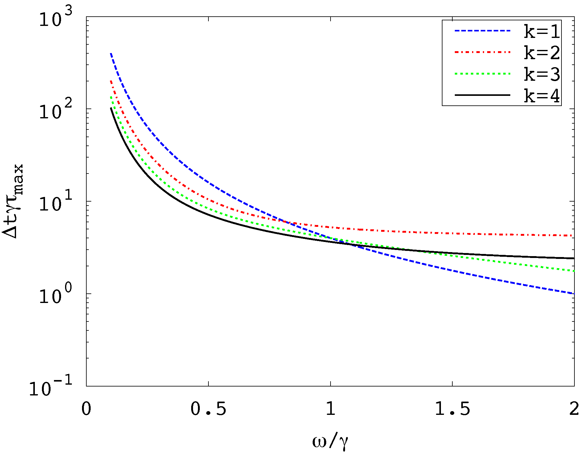
• Figure 1 shows that, for fixed $\mathsf{\Delta }t$ and $\gamma$, the value ${\tau }_{max}^{\left(k\right)}$ is an increasing function of $\omega$, at least for $k=1,2,3,4$. Hence, as for the spectral gap, it is the lowest frequency ${\omega }_1$ that dictates the maximum $\tau$.
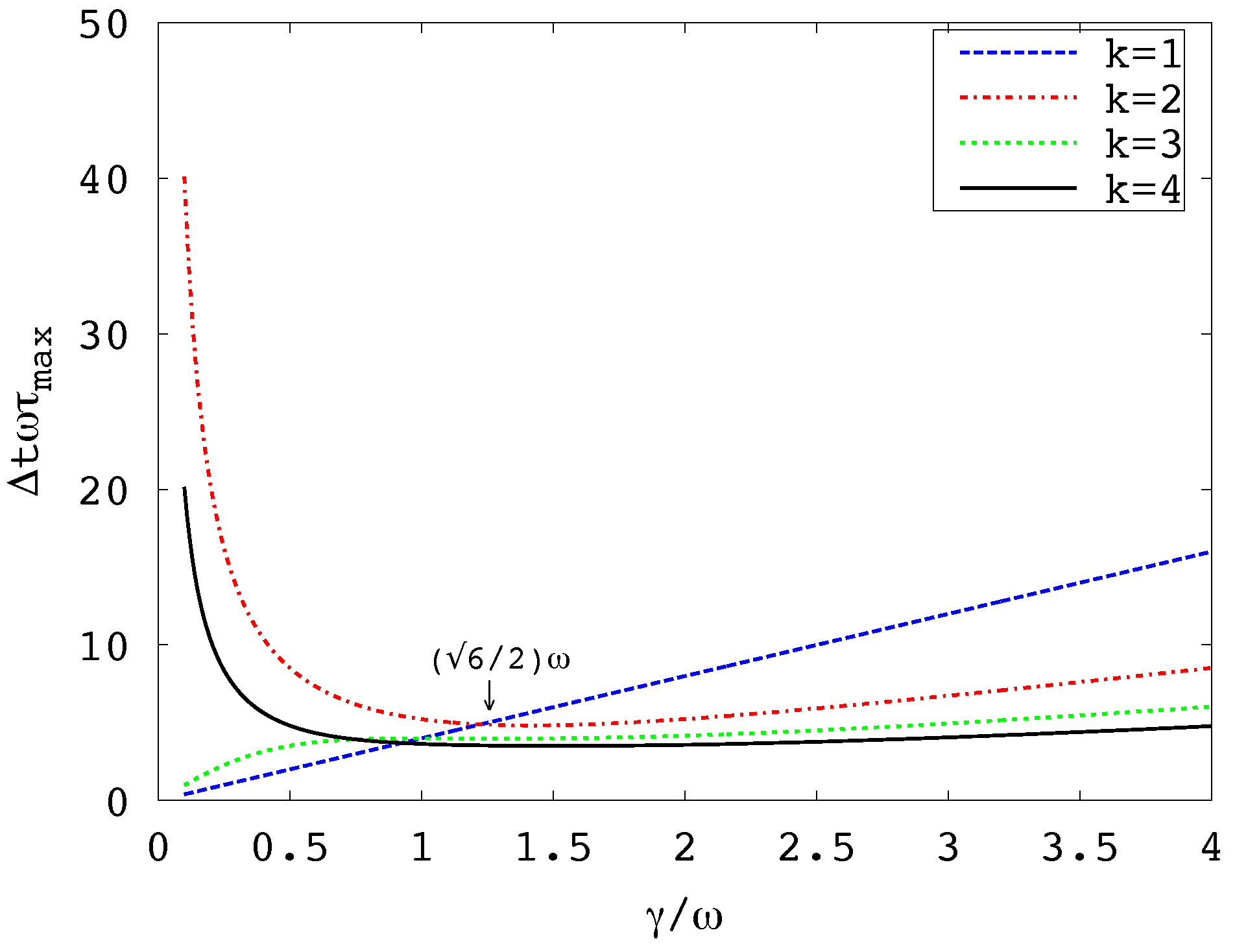
• Figure 2 indicates that, for fixed $\mathsf{\Delta }t$ and $\omega$, the maximizing $\tau$ is either ${\tau }_{max}^{\left(1\right)}$ or ${\tau }_{max}^{\left(2\right)}$, depending on the value of $\gamma$. The optimal damping coefficient is $\gamma =(\sqrt{6}/2)\omega$, for which ${\tau }_{max}^{\left(1\right)}={\tau }_{max}^{\left(2\right)}=\sqrt{6}/\left(\omega \mathsf{\Delta }t\right)$.
• For the preobservable $\omega q$, and, indeed, for any odd polynomial, the IAcT $\tau$ becomes arbitrary small as $\gamma$ goes to zero. This does not mean, however that the variance goes to 0, because Equation (1) is an asymptotic result, and the IAcT is a prefactor for the leading order $1/N$ term in the expression for the variance. The next order $1/N^2$ term would dominate if $\gamma$ were very small. An order $1/N^2$ error is characteristic of uniform sampling, which would be the consequence of nearly ballistic movement. In addition, odd polynomials are special in that their expectation is independent of total energy, so it matters not that barely diffusive movement samples different values of total energy only at a very slow rate.
• The eigenfunction for ${\tau }_{max}^{\left(2\right)}$ is a specific linear combination of ${\omega }^2{q}^2-1$ and $p^2-1$. For quadratic polynomials, the total energy does affect its expected value, which is why it is necessary that $\gamma$ be large enough to sample different energies on a reasonable time scale.

5.1. The Forward Transfer Operator

The forward transfer operator is

$$\mathcal{F}u={\rho }^{-1}{\mathrm{e}}^{\mathsf{\Delta }t{\mathcal{L}}_{\mathrm{K}}}\left(\rho u\right)$$

where

$$\rho (q,p)\propto exp(-\frac{1}{2}{p}^2-\frac{1}{2}{\omega }^2{q}^2).$$

and ${\mathcal{L}}_{\mathrm{K}}$ is the Fokker–Planck operator [14] (Equations (10.1)–(10.3), (10.9))

$${\mathcal{L}}_{\mathrm{K}}f=-p\frac{\partial }{\partial q}f+{\omega }^{2}q\frac{\partial }{\partial p}f+\gamma \frac{\partial }{\partial p}\left(pf\right)+\gamma \frac{{\partial }^2}{\partial p^2}f.$$

Therefore,

$$\mathcal{F}={\mathrm{e}}^{\mathsf{\Delta }t\mathcal{L}}$$

where

$$\mathcal{L}f=\frac{1}{\rho }{\mathcal{L}}_{\mathrm{K}}\left(\rho f\right)=-p\frac{\partial }{\partial q}f+{\omega }^{2}q\frac{\partial }{\partial p}f-\gamma p\frac{\partial }{\partial p}f+\gamma \frac{{\partial }^2}{\partial p^2}f.$$

Using the relation $\mathcal{L}f=\frac{1}{\rho }{\mathcal{L}}_{\mathrm{K}}\left(\rho f\right)$, it is easy to show that the adjoint

$${\mathcal{L}}^{†}f=p\frac{\partial }{\partial q}f-{\omega }^{2}q\frac{\partial }{\partial p}f-\gamma p\frac{\partial }{\partial p}f+\gamma \frac{{\partial }^2}{\partial p^2}f.$$

5.2. Gamma for Maximum Spectral Gap

Ref. [14] (Chapter 10, Equations (1), (2), (3b), (9), (22), (52), (60), (71), (72), (74), (77), (78), (82) and (83)) gives the eigenvalues of ${\mathcal{L}}_K$ as

$${\mu }_{k,l}=-\frac{1}{2}(k+l)\gamma -\frac{1}{2}(k-l)\delta ,k,l=0,1,\dots ,$$

with eigenfunctions

$${\psi }_{k,l}=\rho {(q,p)}^{1/2}{(k!l!{\delta }^{k+l})}^{-1/2}{(\sqrt{{\gamma }_{+}}\mathcal{B}-\sqrt{{\gamma }_{-}}\mathcal{A})}^k{(-\sqrt{{\gamma }_{-}}\mathcal{B}+\sqrt{{\gamma }_{+}}\mathcal{A})}^l\rho {(q,p)}^{1/2},$$

where

$${\gamma }_{\pm }=\frac{1}{2}(\gamma \pm \delta )\text{and}\delta =\sqrt{{\gamma }^2-4{\omega }^2},$$

with the radical sign denoting the principal square root, and operators $\mathcal{A}$, $\mathcal{B}$ defined by

$$\mathcal{A}f=-{\omega }^{-1}\frac{\partial }{\partial q}f+\frac{1}{2}\omega qf,\mathcal{B}f=-\frac{\partial }{\partial p}f+\frac{1}{2}pf.$$

The operator $\mathcal{L}$ has eigenfunctions $\rho {(q,p)}^{-1}{\psi }_{k,l}(q,p)$ and the same eigenvalues; $\mathcal{F}$ has these same eigenfunctions and has eigenvalues $exp\left(\mathsf{\Delta }t{\mu }_{k,l}\right)$. See Ref. [15] for a more general result.

For $k+l=1$, one has ${\mu }_{0,1}=-{\gamma }_{-}$, ${\mu }_{1,0}=-{\gamma }_{+}$ and

$${\phi }_{0,1}={({\gamma }_{-}/\delta )}^{1/2}(-p+{\gamma }_{+}q)\rho (q,p),{\phi }_{1,0}={({\gamma }_{+}/\delta )}^{1/2}(p-{\gamma }_{-}q)\rho (q,p).$$

In the case ${\gamma }_{\pm }=\frac{1}{2}\gamma$, $\mathcal{F}$ has a double eigenvalue ${\lambda }_2={\lambda }_3={\mathrm{e}}^{-\omega \mathsf{\Delta }t}$ but one eigenfunction ${\phi }_2(q,p)=p-\omega q$ and one generalized eigenfunction ${\phi }_3(q,p)=q$, satisfying $(\mathcal{F}-{\lambda }_2){\phi }_3={\phi }_2$. This results in behavior involving a linear combination of ${\mathrm{e}}^{-\omega t}$ and $t{\mathrm{e}}^{-\omega t}$.

The eigenvalue nearest 1 depends on $\mathsf{\Delta }t$. For small enough $\mathsf{\Delta }t$, it is $exp(-{\gamma }_{-}\mathsf{\Delta }t)$, and the spectral gap is $\omega \mathsf{\Delta }t+\mathcal{O}\left(\mathsf{\Delta }{t}^2\right)$ for $\gamma \le 2\omega$ and $\omega \mathsf{\Delta }t(2\omega /\gamma ){(1+{(1-{(2\omega /\gamma )}^2)}^{1/2})}^{-1}+\mathcal{O}\left(\mathsf{\Delta }{t}^2\right)$ otherwise. To maximize the spectral gap, choose $\gamma$ to be no greater than $2\omega$, corresponding to an underdamped system.

5.3. Gamma for Maximum IAcT

To obtain ${\tau }_{max}$, one needs eigenelements for $\mathcal{G}$, given by Equation (2) with $\mathcal{F}=exp\left(\mathsf{\Delta }t\mathcal{L}\right)$. Note that the subspace of polynomials of degree $\le k$ is closed under application of $\mathcal{L}$ and ${\mathcal{L}}^{†}$. Moreover, this holds separately for subspace ${\mathbb{P}}_k$ of odd polynomials of degree $\le k$ for k odd and for subspace ${\mathbb{P}}_k$ of even polynomials of degree $\le k$ for k even. It also applies to operators $\mathcal{E}$, $\mathcal{F}$, ${\mathcal{F}}^{†}$, and $\mathcal{G}$. Hence, the ${\mathbb{P}}_k$ are eigenspaces for $\mathcal{G}$. These eigenspaces can be further decomposed as follows. Let ${\mathbb{P}}_k^{\prime }={\mathbb{P}}_k$ for $k<2$, and let ${\mathbb{P}}_k^{\prime }={\mathbb{P}}_k\cap {\mathbb{P}}_{k-2}^{\perp }$ for $k\ge 2$. The claim is that ${\mathbb{P}}_k^{\prime }$ is an eigenspace, of dimension $k+1$. To confirm this, it is enough to show that $\langle \mathcal{G}u,v\rangle =0$ for any $u\in {\mathbb{P}}_k$, $v\in {\mathbb{P}}_{k-2}$, which follows almost immediately, since ${\mathcal{G}}^{†}=\mathcal{G}$ and $\mathcal{G}v\in {\mathbb{P}}_{k-2}$. Let $\mathbf{u}$ be a basis for ${\mathbb{P}}_k^{\prime }$ chosen so there are even functions of p followed by odd functions of p. In particular,

$$\begin{array}{ccc}\hfill \mathbf{u}& =& {[\omega q,p]}^{\mathsf{T}},\hfill \\ \hfill \mathbf{u}& =& {[{\omega }^2{q}^2-1,\omega qp,p^2-1]}^{\mathsf{T}},\hfill \\ \hfill \mathbf{u}& =& {[{\omega }^3{q}^3-3\omega q,({\omega }^2{q}^2-1)p,\omega q(p^2-1),p^3-3p]}^{\mathsf{T}},\hfill \\ \hfill \mathbf{u}& =& {[{\omega }^4{q}^4-6{\omega }^2{q}^2+3,({\omega }^3{q}^3-3\omega q)p,({\omega }^2{q}^2-1)(p^2-1),\omega q(p^3-3p),p^4-6p+3]}^{\mathsf{T}},\hfill \end{array}$$

for $k=1,2,3,4$, respectively. The polynomials in $\omega q$ and in p are modified versions ${\mathit{He}}_k$ of Hermite polynomials. We have $\mathcal{L}\mathbf{u}=A\mathbf{u}$ for some matrix of constants A, given by

$$A=\left[\begin{array}{cccc}0& -k\omega & & \\ \omega & -\gamma & \ddots & \\ & \ddots & \ddots & -\omega \\ & & k\omega & -k\gamma \end{array}\right].$$

(16)

(cf. Ref. [14], Equations (10.96) and (10.97) for ${\mathcal{L}}_{\mathrm{K}}$.) We have $\mathcal{E}\mathbf{u}=\mathbf{0}$ and ${\mathcal{F}}_0\mathbf{u}=\mathcal{F}\mathbf{u}=exp\left(\mathsf{\Delta }tA\right)\mathbf{u}$. Therefore, from Equations (13) and (14), one has

$$C_k=\langle {\mathcal{F}}_0^k\mathbf{u},{\mathbf{u}}^{\mathsf{T}}\rangle =exp\left(k\mathsf{\Delta }tA\right)\langle \mathbf{u},{\mathbf{u}}^{\mathsf{T}}\rangle ,$$

and

$$K=coth(-\frac{1}{2}\mathsf{\Delta }tA)\langle \mathbf{u},{\mathbf{u}}^{\mathsf{T}}\rangle =coth(-\frac{1}{2}\mathsf{\Delta }tA)C_0.$$

For each value of k, ${\tau }_{max}$ is the maximum eigenvalue of

$$\frac{1}{2}\left(C_0^{-1}coth(-\frac{1}{2}\mathsf{\Delta }tA)C_0+coth{(-\frac{1}{2}\mathsf{\Delta }tA)}^{\mathsf{T}}\right).$$

(17)

As explained in Section 3.1, if the basis functions are re-ordered so that those that are even functions of p precede those that are odd functions of p, the eigenvalue problem splits into two nearly equal parts.

For $k=1$, $A=X\mathrm{\Lambda }{X}^{-1}$ where $\mathrm{\Lambda }=\mathrm{diag}(-{\gamma }_{-},-{\gamma }_{+})$ and

$$X=\left[\begin{array}{cc}\omega & \omega \\ {\gamma }_{-}& {\gamma }_{+}\end{array}\right].$$

The covariance matrix $C_0=\langle \mathbf{u},{\mathbf{u}}^{\mathsf{T}}\rangle =\mathrm{diag}(1,1)$, and matrix (17) is $\mathrm{diag}({\tau }_{+},{\tau }_{-})$ where

$${\tau }_{\pm }=\frac{1}{\delta }\left(\pm {\gamma }_{\pm }coth(\frac{1}{2}\mathsf{\Delta }t{\gamma }_{-})\mp {\gamma }_{\mp }coth(\frac{1}{2}\mathsf{\Delta }t{\gamma }_{+})\right).$$

Using the identity $coth(x\pm y)=(sinh2x\mp sinh2y)/(cosh2x-cosh2y)$, one gets that the eigenvalues of matrix (17) are

$${\tau }_{\pm }=\frac{sinh\left(\frac{1}{2}\mathsf{\Delta }t\gamma \right)\pm \gamma sinh\left(\frac{1}{2}\mathsf{\Delta }t\delta \right)/\delta }{cosh\left(\frac{1}{2}\mathsf{\Delta }t\gamma \right)-cosh\left(\frac{1}{2}\mathsf{\Delta }t\delta \right)}.$$

The greater of ${\tau }_{\pm }$ is ${\tau }_{+}$, and it is a straightforward exercise to show that ${\tau }_{+}$ is an decreasing function of $\omega$ as long as

$${\left(\omega \mathsf{\Delta }t\right)}^2\le {\pi }^2+{(\gamma \mathsf{\Delta }t/2)}^2.$$

(18)

In practice, a numerical integrator is used, whose step size is chosen so that $\mathsf{\Delta }tL=\theta$ where $\theta$ is some fractional value, e.g., $\frac{1}{2}$, and L is the magnitude of largest eigenvalue of the Jacobian matrix of the right-hand side of the system of (first-order) stochastic differential equations. In particular,

$$\omega \mathsf{\Delta }t=\theta \mathrm{if}\gamma \le 2\omega ;$$

(19)

otherwise, it holds that $\omega \mathsf{\Delta }t<\gamma \mathsf{\Delta }t/2$. Hence, Inequality (18) is more than satisfied. It is more complicated to analyze the behavior of values of $\tau$ for $k>1$, so we exploit the smallness of $\omega \mathsf{\Delta }t$ and $\gamma \mathsf{\Delta }t$ to do an asymptotic analysis. From Expression (17), one sees that for ${\mathbb{P}}_k^{\prime }$, its ${\tau }_{max}$ equals ${\tau }_{max}^{\left(k\right)}+\mathcal{O}\left(\mathsf{\Delta }t\right)$ where ${\tau }_{max}^{\left(k\right)}$ is the greatest eigenvalue of

$$-\frac{1}{\mathsf{\Delta }t}(C_0^{-1}{A}^{-1}{C}_0+A^{-\mathsf{T}}).$$

(20)

For $k=1$, one has $C_0=\mathrm{diag}(1,1)$ and ${\tau }_{max}^{\left(1\right)}=2\gamma /\left({\omega }^2\mathsf{\Delta }t\right)$, corresponding to the eigenfunction $\omega q$. For $k=2$, one has

$$A^{-1}=\frac{1}{2\gamma {\omega }^2}\left[\begin{array}{ccc}-{\gamma }^2-{\omega }^2& 2\gamma \omega & -{\omega }^2\\ -\gamma \omega & 0& 0\\ -{\omega }^2& 0& -{\omega }^2\end{array}\right],$$

$C_0=\mathrm{diag}(2,1,2)$, and the largest eigenvalue for Expression (20) is

$${\tau }_{max}^{\left(2\right)}=\frac{1}{2\mathsf{\Delta }t}\left(\frac{\gamma }{{\omega }^2}+\frac{2}{\gamma }+\sqrt{\frac{{\gamma }^2}{{\omega }^4}+\frac{4}{{\gamma }^2}}\right),$$

corresponding to an eigenfunction that is some linear combination of ${\omega }^2{q}^2-1$ and $p^2-1$. Again ${\tau }_{max}^{\left(k\right)}$ is a decreasing function of $\omega$ for small enough $\mathsf{\Delta }t$. For general k, the size of the elements of A in Equation (16) increase with $\omega$, which suggests that for practical values of $\mathsf{\Delta }t$, the largest eigenvalue for Expression (20) decreases with $\omega$. This can be confirmed numerically. To reduce the number of parameters, write $A=-\omega B(\gamma /\omega )$, and rewrite Expression (20) as

$$\frac{1}{\omega \mathsf{\Delta }t}(C_0^{-1}B{(\gamma /\omega )}^{-1}{C}_0+B{(\gamma /\omega )}^{-\mathsf{T}}).$$

(21)

The value ${\tau }_{max}^{\left(k\right)}$ is the largest eigenvalue of Matrix (21), so $\gamma \mathsf{\Delta }t{\tau }_{max}^{\left(k\right)}$ is a function only of the ratio $\omega /\gamma$. Figure 1 plots this quantity for $k=1,2,3,4$, confirming that ${\tau }_{max}^{\left(k\right)}$ is decreasing function of $\omega$ for fixed values of $\gamma$ and $\mathsf{\Delta }t$.

Therefore, for a multidimensional quadratic potential, ${\tau }_{max}$ is very likely to be determined by the lowest frequency mode. (This is readily established for the spectral gap for reasonable values of $\mathsf{\Delta }t$.)

Having established that the lowest frequency mode is most likely responsible for ${\tau }_{max}$, let $\omega$ denote the lowest frequency ${\omega }_1$, and consider the optimal choice of $\gamma$. From Matrix (21), observe that $\omega \mathsf{\Delta }t{\tau }_{max}^{\left(k\right)}$ is a function only of $\gamma /\omega$. Accordingly, we choose $\gamma /\omega$ to minimize ${max}_k\omega \mathsf{\Delta }t{\tau }_{max}^{\left(k\right)}$. However, $\mathsf{\Delta }t$ may depend on $\gamma$, but only if $\gamma >2{\omega }_{\nu }$, according to Equation (19). Let us initially ignore this possibility and revisit it after determining the optimal $\gamma$.

Assuming that the maximum of $\omega \mathsf{\Delta }t{\tau }_{max}^{\left(k\right)}$ is attained for $k=1$ or $k=2$, there are two possible locations for the best $\gamma$. One is the choice $\gamma =\sqrt{2}\omega$, for which $\omega \mathsf{\Delta }t{\tau }_{max}^{\left(2\right)}=1+\sqrt{2}$ and $\omega \mathsf{\Delta }t{\tau }_{max}^{\left(1\right)}=2\sqrt{2}$. The other is the choice $\gamma =(\sqrt{6}/2)\omega$ where $\omega \mathsf{\Delta }t{\tau }_{max}^{\left(k\right)}=\sqrt{6}$ for both $k=1$ and $k=2$. The latter is the better choice. This and the assumption that the maximum occurs for $k<3$ is supported by Figure 2, which plots ${\tau }_{max}$ as a function of $\gamma$ for fixed values of $\omega$ and $\mathsf{\Delta }t$. Since $(\sqrt{6}/2){\omega }_1<2{\omega }_{\nu }$, we see from Equation (19) that there is no concern about $\mathsf{\Delta }t$ limiting the value of $\gamma$.

Note that for the optimal $\gamma$, the dynamics is underdamped in every mode.

6. Discussion and Conclusions

It is asserted in the literature [1,4] that, for comparing MCMC propagators and for ensuring reasonably reliable simulation results, it is of great value to estimate the maximum autocorrelation time over all possible observables. Certainly, this would seem desirable for comparing propagators, since it is best to assume as little as possible about the actual observables that are to be estimated from the Markov chain. In addition, the longest IAcT would be more reliably estimated than any other IAcT, because its accurate estimation would call for a greatest number of samples; moreover, the accuracy of estimates of other IAcTs might be influenced by the longest IAcT. Unfortunately, estimating IAcTs and assessing such estimates is a difficult task, which can benefit greatly from further research.

In this article, it is suggested that the maximum IAcT be estimated by considering an arbitrary linear combination of basis functions chosen to capture the lowest frequency motions of the dynamics of the MCMC chain. It is also worth considering the approach based on a set of well chosen indicator functions [11].

Another quantity for measuring performance of an MCMC propagator is the spectral gap. It is related to equilibration time, but as a predictor of IAcTs, it can be arbitrarily too pessimistic or it can be too optimistic. Such is the case for irreversible propagators, especially for energy landscapes where entropy barriers dominate energy barriers.

Shorter integrated autocorrelation times are thus a primary consideration in the design of MCMC propagators. Simple examples are constructed to explain how irreversibility might help, though their relevance to practical propagators is unclear. Nonetheless, it is advantageous not to insist on reversibility. In particular, the ballistic component of propagators like hybrid Monte Carlo and Langevin dynamics may offer dramatic speedups for overcoming entropy barrriers, though no advantage for energy barriers.

Irreversible propagators typically have a parameter that determines the extent of diffusive behavior. For discrete Langevin dynamics applied to a multidimensional quadratic potential, the optimal value corresponds to slightly underdamped dynamics for the lowest frequency mode, with other modes experiencing even lighter dampling. However, this conclusion is not necessarily indicative of the optimal damping for the usual situation, in which there a multiplicity of energy minima, and further studies are needed.

In a nutshell, general-purpose sampling benefits greatly from the use of irreversible propagators in extended state space, with “diffusion parameter(s)” chosen to minimize the maximum integrated autocorrelation time, which for a quadratic potential energy corresponds to moderately underdamped dynamics in the lowest frequency mode.

References

- Fang, Y.; Cao, Y.; Skeel, R. Quasi-Reliable Estimates of Effective Sample Size. arXiv, 2017; arXiv:1705.03831v2. [Google Scholar]
- Schütte, C.; Huisinga, W. Biomolecular Conformations as Metastable Sets of Markov Chains. In Proceedings of the 38th Annual Allerton Conference on Communication, Control, and Computing, Monticello, IL, USA, 4–6 October 2000; pp. 1106–1115. [Google Scholar]
- Schütte, C.; Sarich, M. Metastability and Markov State Models in Molecular Dynamics; American Mathematical Society: Providence, RI, USA, 2013. [Google Scholar]
- Lyman, E.; Zuckerman, D.M. On the Structural Convergence of Biomolecular Simulations by Determination of the Effective Sample Size. J. Phys. Chem. B 2007, 111, 12876–12882. [Google Scholar] [CrossRef] [PubMed]
- Rey-Bellet, L.; Spiliopoulos, K. Irreversible Langevin Samplers and Variance Reduction: A Large Deviations Approach. Nonlinearity 2015, 28, 2081–2104. [Google Scholar] [CrossRef]
- Leimkuhler, B.; Matthews, C. Rational Construction of Stochastic Numerical Methods for Molecular Sampling. Appl. Math. Res. Express 2013, 2013, 34–56. [Google Scholar] [CrossRef]
- Leimkuhler, B.; Matthews, C.; Stoltz, G. The Computation of Averages from Equilibrium and Nonequilibrium Langevin Molecular Dynamics. IMA J. Numer. Anal. 2016, 36, 13–79. [Google Scholar] [CrossRef]
- Geyer, C.J. Practical Markov Chain Monte Carlo. Stat. Sci. 1992, 7, 473–511. [Google Scholar] [CrossRef]
- Priestly, M.B. Spectral Analysis and Time Series; Academic Press: Cambridge, MA, USA, 1981. [Google Scholar]
- Goodman, J. Acor, Statistical Analysis of a Time Series. 2009. Available online: http://www.math.nyu.edu/faculty/goodman/software/acor/ (accessed on 4 August 2014).
- Zhang, X.; Bhatt, D.; Zuckerman, D.M. Automated Sampling Assessment for Molecular Simulations Using the Effective Sample Size. J. Chem. Theory Comput. 2010, 6, 3048–3057. [Google Scholar] [CrossRef] [PubMed]
- Cancés, E.; Legoll, F.; Stoltz, G. Special Issue on Molecular Modelling: Theoretical and Numerical Comparison of Some Sampling Methods for Molecular Dynamics. ESAIM Math. Model. Numer. Anal. 2007, 41, 351–389. [Google Scholar] [CrossRef]
- Diaconis, P.; Holmes, S.; Neal, R.M. Analysis of a Nonreversible Markov Chain Sampler. Ann. Appl. Probab. 2000, 10, 726–752. [Google Scholar] [CrossRef]
- Risken, H. The Fokker-Planck Equation. Methods of Solution and Applications; Springer Series in Synergetics; Springer: New York, NY, USA, 1984; Volume 18. [Google Scholar]
- Kozlov, S. Effective diffusion for the Fokker-Planck equation. Math. Notes 1989, 45, 360–368. [Google Scholar] [CrossRef]