Multiple Discrete Endogenous Variables in Weakly-Separable Triangular Models

Abstract

We consider a model in which an outcome depends on two discrete treatment variables, where one treatment is given before the other. We formulate a three-equation triangular system with weak separability conditions. Without assuming assignment is random, we establish the identification of an average structural function using two-step matching. We also consider decomposing the effect of the first treatment into direct and indirect effects, which are shown to be identified by the proposed methodology. We allow for both of the treatment variables to be non-binary and do not appeal to an identification-at-infinity argument.

1. Introduction

This paper deals with nonparametric identification in a three-equation nonparametric model with discrete endogenous regressors. We provide conditions under which an average structural function (ASF) (e.g., [1]) is point identified and discuss how different treatment effects can be identified using our methods. Like [2,3], we use a Dynkin system approach, which is based on the idea of matching; the idea of matching was also used by [3,4] inter alia, albeit that our notion of matching is different from the commonly-used matching method in the treatment effect literature (e.g., [5]). The latter uses the matching idea to control for observed covariates, while our method matches on identified/estimable sets, i.e., elements of Dynkin systems, as will become apparent below.

To motivate the parameter of interest in this paper, consider the example of assessing the dynamic evolution of crime (e.g., [6]). The number of crimes, say murders, at time t is affected both by the number of crimes prior to time t and by the level of police activity (measured by, e.g., the number of police patrols) at time t. This example has a special triangular structure, because the number of police patrols at time t is in part a response to the number of crimes at time $t-1$. The number of crimes is discrete, as is the number of police patrols. There are several potential endogeneity problems in this example, e.g., simultaneity between crimes and police activity at time t and unobserved heterogeneity due to changes in the neighborhood and its surroundings. We focus on the identification of the ASF, which in this example, corresponds to the mean number of crimes at time t that would occur if both the number of crimes at time $t-1$ and the number of police patrols were exogenously fixed. There are other objects of potential interest that can be identified with our identification strategy. For instance, one could instead fix the number of crimes at time $t-1$, but allow the number of police patrols to respond to it endogenously. We can thus decompose the effect of the changes of the past number of crimes into a direct effect and an indirect effect: a high level of crime at time $t-1$ can create an environment in which crime thrives at time t (e.g., because criminals build up local knowledge, set up networks), but it also leads to an increased police presence, which reduces crimes at time t. We also discuss such decompositions in this paper.

The model that we study is similar to that in [3,4] and others in that we make and exploit a weak separability assumption. However, [4] specifically excludes the possibility of non-binary categorical endogenous regressors, imposes restrictive support conditions on the covariates and only deals with the two-equation case. The non-binary categorical regressor case is not discussed in (the published version of) [3], which further does not deal with the present, more complicated, three-equation model featuring two discrete endogenous regressors. In this paper, we show that the methodology developed in [3] can be used to study non-binary treatments with a double layer of endogeneity. There are other papers that have a three-equation model and/or allow for non-binary regressors (e.g., [7,8,9]), but the model or the object of interest is generally different.

There are many examples in which (a (semi)parametric version of) our structure has been used. We mention only a few. The work in [10] studies the effects of smoking on birth weight through the mechanism of gestation time. The work in [11] analyzes the effects of school type and class size on earnings and educational attainment. The work in [12] has a simpler dependence structure than the one used here. The work in [13] investigates labor market returns to community college attendance and four-year college education. The work in [14] considers the multi-stage nature of the adoption process of on-line banking services, where interruptions in the initial sign-up stage and in the later regular use stage are the treatments of interest. We further note that the double hurdle model of [15], which is used in much empirical work, is a special case of our model, albeit that the identification methods developed here are of limited use in Cragg’s specification.

The focus here is on point identification. There are several papers (e.g., [16,17,18]) that develop bounds on treatment effects in models that are similar to, but simpler than, the one in this paper using weaker monotonicity assumptions than are imposed here. As shown in [2], the Dynkin system approach can be used to obtain sharp bounds in an environment in which there is only partial identification. We do not pursue this possibility in the current paper.

Identification of parameters of interest in our paper proceeds in two steps. In the first step, we use the variation in the instrument $z$ for the treatment $d$ to infer what variation in the instrument for the intermediate endogenous variable $s$ would compensate exactly for variation in $d$. Using this information, we can undo the effect of changing $d$ on $s$. Provided that the instruments for $d$ and $s$ have sufficient variation, we can identify the structural function for $s$ this way. Using this first stage information along with variation in instruments for $d$ and $s$, we infer what variation in the exogenous regressors in the outcome equation would compensate exactly for variation in both treatment $d$ and intermediate endogenous variable $s$. Our paper differs from both [2,3,4] in that we have to use another level of matching in order to undo the effect of both $d$ and $s$ on the outcome $y$. A critical component of our strategy is the existence of instruments for the endogenous regressors $d$ and $s$ and sufficient variation in the exogenous regressors in the outcome equation to allow us to compensate for variation in the endogenous regressors directly.

The Dynkin system approach is a natural scheme that allows one to collect and aggregate information contained in the data in a natural and thorough fashion through a recursion scheme1. Each combination of observables implies that the unobservable error terms belong to certain sets. From these sets, one can infer additional information through various operations on these sets. In this paper, we use a version of the Dynkin system approach, first used in [3], which exploits matching in addition to the union and difference operators used in [2]. Matching has been used frequently in the past. For instance, [20] used it to avoid support conditions in estimating weakly-separable nonparametric regression functions. The way we use matching in this paper is closer to [4], albeit that our procedure, as already mentioned, can be applied more generally.

Although the fact that the Dynkin system approach requires only weak covariate support restrictions is an attractive feature, this paper will instead focus on extending the use of the Dynkin system to more complicated situations, since the support restrictions issue was discussed at length in [3], albeit for the two-equation binary endogenous regressor case. Further, the Dynkin system mechanism can be used to study effects other than average partial effects, such as marginal treatment effects (e.g., [21]), but here, we focus on average partial effects.

The remainder of the paper is organized as follows. In Section 2, we lay out our model and discuss the objects we want to identify and the rationale for our desire to do so. Section 3 provides a rough description of the basic ideas underlying our identification approach. These ideas are formalized and illustrated using more complete examples in Section 4 and Section 5. Finally, Section 7 provides a brief sketch of how the identification methods proposed here could be implemented.

2. Model

Imposing weak separability in multiple places, we consider the model

$$\left\{\begin{array}{c}y=g(\alpha (x,s,d),ϵ),\hfill \\ s=\sum _{j=1}^{{\eta }_s}\{v>m_j(x,w,d)\},\hfill \\ d=\sum _{j=1}^{{\eta }_d}\{u>p_j(x,w,z)\},\hfill \end{array}\right.$$

(1)

where ${\eta }_s,{\eta }_d\ge 1$ and $g,m_1,\dots ,m_{{\eta }_s},p_1,\dots ,p_{{\eta }_d}$ are unknown functions. We assume that ${\eta }_s,{\eta }_d$ are known and that we observe $y,s,d,x,w,z$. The unobservables $u$ and $v$ are scalar random variables; the dimension of $ϵ$ is not restricted.

One feature in (1) is that $w$ and $z$ are excluded from the first and second equations, respectively. Our identification arguments will require that $w$ and $z$ be able to vary the $m_j$ and $p_j$ functions, respectively, but the fact that $x$ appears in the $m_j$ functions and $x,w$ do in the $p_j$ functions will be immaterial. Therefore, we will simply consider

$$\left\{\begin{array}{c}y=g(\alpha (x,s,d),ϵ),\hfill \\ s=\sum _{j=1}^{{\eta }_s}\{v>m_j(w,d)\},\hfill \\ d=\sum _{j=1}^{{\eta }_d}\{u>p_j(z)\},\hfill \end{array}\right.$$

(2)

for the sake of illustrational clarity. We now impose that $p_0(z)=m_0(w,d)=0$, $p_j(z)<p_{j+1}(z)$, $m_j(w,d)<m_{j+1}(w,d)$ and $p_{{\eta }_d+1}(z)=m_{{\eta }_s+1}(w,d)=1$. This is without loss of generality in view of Assumption B below. The setup in (2) requires that the exogenous covariates $x,w,z$ appear only once in each equation2. It is straightforward to generalize our identification strategy to Model (1) at the expense of exposition. However, doing so would introduce additional notational complexity and requires more variations in $w$ and $z$.

In the crime example discussed in the Introduction, $y$ would be the number of crimes this period, $s$ the number of police patrols and $d$ the number of crimes in the previous period. Then, $x,z$ represent observable exogenous neighborhood characteristics this period and last period, respectively. Finally, $w$ can contain variables that reflect the resources that the police can employ to combat crime, with the implicit assumption that such resources cannot be enhanced in the short term and can hence be treated as exogenous.

We now make several model assumptions. Let $\mathcal{U}=(0,1]$.

Assumption A. $(u,v,ϵ)$ is independent of $(w,z,x)$.

Assumption B. The distribution of $(u,v)$ is absolutely continuous with respect to the Lebesgue measure μ with support ${\mathcal{S}}_{uv}={\mathcal{U}}^2$, and $u,v$ have marginal uniform distributions on $\mathcal{U}$.

Assumption C. $\mathbb{E}[g(\alpha ,ϵ)|u=u,v=v]$ is for all $u,v\in \mathcal{U}$ strictly monotonic in α.

Assumption A is strong, but can be relaxed to independence conditional on covariates, i.e., either covariates in addition to $w,z,x$ or elements of vector-valued $w,z,x$. Moreover, if g is additively separable in $ϵ$, then Assumption A can be further weakened as explained below.

The second half of Assumption B constitutes a normalization. The first part is restrictive, but is difficult to avoid. Please note, however, that $u$ and $v$ are allowed to be dependent and that the support of $(u,v)$ given $ϵ$ need not be ${\mathcal{U}}^2$.

Monotonicity is a common assumption in the nonparametric identification literature, but unlike, e.g., [22,23,24], Assumption C does not require monotonicity in the error term of the structural function g itself, but instead, it requires monotonicity of the (conditional) expectation3; a similar assumption can be found in [4]. For instance, an indicator function, such as $g(\alpha ,ϵ)=\{ϵ>\alpha \}$, is allowed, as long as $ϵ$ is continuously distributed, given $u$ and $v$. However, the single index feature of the structural function is an essential feature of Assumption C. For the use of the Dynkin system idea to identify a structural function under a stronger form of monotonicity, see [2].

Both $s$ and $d$ are general ordered response variables, which are allowed to be endogenous. Instead of having one variable with $(1+{\eta }_s)(1+{\eta }_d)$ support points, we have two treatment variables here4 that depend on two distinct error terms, $u$ and $v$. As a result, if we tried to combine $s$ and $d$ into one variable with $(1+{\eta }_s)(1+{\eta }_d)$ support points, the resulting random variable would not necessarily have the threshold crossing form that $s$ and $d$ have in our paper. This is because to have a treatment variable that has a threshold crossing form, $u$ and $v$ would have to be represented by a single unobservable, whose values could be ordered linearly. However, there does not generally exist such a one-to-one mapping. Without having a discrete treatment variable that has this threshold crossing form, the identification method given in [4] would not work. Since [3] also consider a single treatment variable with a threshold crossing form, the method in [3] would not work either. As a result, the model studied in this paper is not covered by the models studied in [3,4]. It is also more general than the double hurdle model of [15], Equations (5) and (6), albeit that our matching strategy for identification is of limited usefulness there5.

When discussing our assumptions, we mentioned that Assumption A could be weakened further if g is additively separable in $ϵ$. To be more specific, let $x={(x_1,x_2^{\top })}^{\top },w={(w_1,x_2^{\top })}^{\top }$ and $z={(z_1,x_2^{\top })}^{\top }$, where $x_1,w_1,z_1$ are scalar-valued random variables. Suppose that the outcome equation is given by

$$y=h(x_2,s,d)+x_1\beta +ϵ,$$

(3)

which is a form commonly applied by researchers. Then, Assumption A can be further weakened in the following way:

Assumption D. (i) $ϵ=x_1\gamma +\widetilde{ϵ}$, (ii) $\mathbb{E}(\widetilde{ϵ}|u,v,w_1,z_1,x_1,x_2)=\mathbb{E}(\widetilde{ϵ}|u,v,x_2)$, (iii) $(u,v)$ is independent of $(x_1,w_1,z_1)$ conditional on $x_2$ and (iv) $\beta +\gamma \ne 0$.

Under Assumption D, the outcome Equation (3) can be written as

$$y=h(x_2,s,d)+x_1(\beta +\gamma )+\widetilde{ϵ},$$

(4)

and $\beta +\gamma$ can be identified by running an OLS regression of $y-\mathbb{E}(y|x_2,d,s,w_1,z_1)$ on $x_1-\mathbb{E}(x_1|x_2,d,s,w_1,z_1)$, since

$$\mathbb{E}(y|x_2,d,s,w_1,z_1)=h(x_2,s,d)+\mathbb{E}(x_1|x_2,d,s,w_1,z_1)(\beta +\gamma )+\rho (x_2,d,s,w_1,z_1)+e,$$

where $\rho (x_2,d,s,w_1,z_1)=\mathbb{E}(\widetilde{ϵ}|x_2,d,s,w_1,z_1)$. Then, $x_1(\beta +\gamma )$ can be used to compensate for the effects of varying $d$ and $s$ in the outcome equation as long as $\beta +\gamma \ne 0$.

To see why this weakening of Assumption A might be particularly useful, suppose that $y$ equals adult wages of an individual, treatment $d$ is whether a student is assigned to a small class or not and $s$ is an indicator for college attendance. This example is also considered in [25]. The instrument for $d$ is the educational intervention in the Project STAR experiment, in which early graders were randomized into small classes, and the instrument for $s$ could be the variation in tuition fees or distance to college; see, for instance, [13,26]. We still need a variable in the wage equation that is exogenous and that does not enter the other two equations. Under Assumption D, the exogeneity condition such a variable has to satisfy is considerably weaker than the one embodied in Assumption A. In particular, the individual’s age when adult wage is measured might be a reasonable candidate as the required $x_2$.

In contrast to the existing literature, including [3,4], which mainly focuses on the effects of one endogenous variable while fixing other variables, our setting features multiple endogenous treatments with a triangular structure, which allows us to consider various causal parameters, such as direct and indirect (average) effects of the treatment variable $d$. Below, we discuss such parameters and methods of identifying them, albeit that our main focus is on identifying the average structural function.

We now formally state the average structural function we analyze. Let $y_{sd}=g(\alpha (x,s,d),ϵ)$. Thus, $y_{sd}=y$ if $(s,d)=(s,d)$, but if $(s,d)\ne (s,d)$, then $y_{sd}$ is the value $y$ would have taken if the same individual had $s=s,d=d$. Therefore, $y_{sd}$ is a typical counterfactual outcome variable, but with two indices instead of the usual one. The focus in this paper will be on the identification of

$$\psi (x^{*},s^{*},d^{*})=\mathbb{E}(y_{s^{*}{d}^{*}}|x=x^{*})=\mathbb{E}g(\alpha (x^{*},s^{*},d^{*}),ϵ),$$

(5)

where $x^{*},s^{*},d^{*}$ are chosen by the researcher. We obtain identification of $m_s(w,d)$ as a byproduct. Please note that $\psi (x^{*},s^{*},d^{*})$ is the ASF conditional on $x=x^{*}$, when the treatments are exogenously fixed at $s^{*}$ and $d^{*}$. For instance, $\psi (1,1,1)$ could be the counterfactual mean earnings of a male worker ($x=1$) if he had both a college degree ($d=1$) and received on-the-job training ($s=1$), or it could be the counterfactual mean birth weight for an infant if her mother had a normal gestation length ($s=1$) and smoked ($d=1$). In the crime example, $\psi (1,1,1)$ is the mean number of crimes at time t if current neighborhood characteristics $x$ are one and with both police patrols at time t and crime at $t-1$ for exogenous reasons.

The function ψ can be used to obtain many, but not all, causal effects of interest. Recall the dual binary treatment example involving college education and on-the-job training. Consider exogenously changing $d$ and fixing $s$ at a specified value $s^{*}$. Then, one can identify the ceteris paribus effect of a change in college education status on earnings for a male worker with job training, i.e., $\psi (1,s^{*},1)-\psi (1,s^{*},0)$. We call this an average partial treatment effect. Alternatively, we can define average joint treatment effects by looking at the causal effects on earnings for male workers of exogenously changing both college education and job training status, i.e., $\psi (1,1,1)-\psi (1,0,0)$. One can aggregate up such effects across sexes, or indeed across job training statuses, e.g., $\mathbb{E}\left[\psi (1,\tilde{s},1)-\psi (1,\tilde{s},0)\right]$, where $\tilde{s}$ is drawn from a suitable job training status distribution.

It should also be noted that our results can be further used to conduct a decomposition of direct and indirect effects for policy analysis. For instance, if the policy maker can only influence college education decisions, but not job training decisions directly, then an object of interest would be the effect of exogenously changing $d$ on a male worker’s mean earnings leaving $s$ to adjust according to the preferences of the worker and his employer, i.e., the parameter

$$\begin{array}{c}\mathbb{E}g\left(\alpha (x,s_1(w),1),ϵ\right)-\mathbb{E}g\left(\alpha (x,s_0(w),0),ϵ\right)\hfill \\ \hfill =[\mathbb{E}g\left(\alpha (x,s_1(w),1),ϵ\right)-\mathbb{E}g\left(\alpha (x,s_1(w),0),ϵ\right)]\hfill \\ \hfill +[\mathbb{E}g\left(\alpha (x,s_1(w),0,ϵ\right)-\mathbb{E}g\left(\alpha (x,s_0(w),0),ϵ\right)],\end{array}$$

(6)

where $s_d(w)$ is the counterfactual value of $s$ when $d$ is exogenously fixed at d given $w=w$6. We call the left-hand side in (6) an average total treatment effect, which is decomposed into a direct effect and an indirect effect on the right-hand side7. Although the parameters in (6) are not represented by ψ, the methods we develop to identify ψ can be used to identify them, as we show in Section 6.

The fact that there are several causal parameters of potential interest arises both because there are multiple endogenous treatment variables and because of the triangular nature of the model. However, we do not believe that one parameter is generally more important than others, but the purpose and context of the policy question of interest should be taken into account. As explained in Section 6, identification of causal parameters, like (6), can be established by the matching method developed in this paper. Therefore, we focus on the identification of ψ (and $m_s$) in the main text to highlight the idea of matching, while we show in Section 6 that the identification of (6) can be obtained by the same methods.

3. Description

We now provide a broad and rough description of our identification strategy. We combine the idea of matching to that of set operations. Matching was also used in [3,4], inter alia. Indeed, our methodology shares some of the intuition with Jun, Pinkse, and Xu (2012) [3]: this will become clear as we proceed. However, due to the triangular structure, the procedure used in this paper is more complicated than that in [3]. The methodology in [3] covers the specification in [4] as a special case.

There are several unknown functions in our model: the $p_j$’s, $m_j$’s and α are important to identify ψ. The $p_j$ functions are identified directly from the data since $p_j(z)$ is simply the probability that the number of crimes last period was no more than $j-1$ given that $z=z$. Identification of the $m_j$’s is more involved, but is simpler than that of ψ. Therefore, we start with the $m_j$ functions.

Our method of identifying the $m_j$’s is related to the identification approaches in [3,4]. Indeed, if $d$ is binary and the joint support ${\mathcal{S}}_{wz}$ of $(w,z)$ is sufficiently rich, then our approach has the same intuition as that in [4]. For instance, we also ask what changes in police resources will offset the changes in police activity induced by changes in the number of past crimes. However, the method of [4] only applies to the case in which $d$ is binary. Below, we explain how matching is convenient when $d$ is binary and how our Dynkin system can be used to obtain identification if $d$ is not necessarily binary.

We start with the simple case, i.e., binary $d$. Consider the problem of identifying $m_1(w^{*},0)$. Note that for any value of z,

$$\begin{array}{cc}\hfill m_1(w^{*},0)=\mathbb{P}(v\le & m_1(w^{*},0))\hfill \\ & =\underset{=\mathbb{P}(s=0,d=0|w=w^{*},z=z)}{\underbrace{\mathbb{P}\left(v\le m_1(w^{*},0),0<u\le p_1(z)\right)}}+\mathbb{P}\left(v\le m_1(w^{*},0),p_1(z)<u\le 1\right).\hfill \end{array}$$

(7)

Note here that the inequality $v\le m_1(w^{*},0)$ describes the event in which the potential status of $s$ given $w=w^{*}$ when $d$ is fixed at zero is equal to zero. There are two possibilities: either $d$ is actually equal to zero (the first right-hand side term in (7)) or it is not equal to zero (the second right-hand side term in (7)). The first right-hand side term in (7) can be inferred directly from the distribution of observables and is hence identified. This is where matching is useful. If we can find $\tilde{w}$ such that $m_1(w^{*},0)=m_1(\tilde{w},1)$, then $v\le m_1(w^{*},0)$ is the same event as $v\le m_1(\tilde{w},1)$. Therefore, the second term on the right-hand side of (7) equals

$$\mathbb{P}\left(v\le m_1(\tilde{w},1),p_1(z)<u\le 1\right)=\mathbb{P}(s=0,d=1|w=\tilde{w},z=z).$$

The question is how to find such $\tilde{w}$. The work in [4] proposes finding $\tilde{w}$ for which the left-hand sides (and therefore, the right-hand sides) in the following equations are equal.

$$\begin{array}{cc}\hfill \mathbb{P}(s=0,d=0|w=w^{*},z=\tilde{z})-\mathbb{P}(s=0,d& =0|w=w^{*},z=z)\hfill \\ & =\mathbb{P}\left(v\le m_1(w^{*},0),p_1(z)<u\le p_1(\tilde{z})\right),\hfill \end{array}$$

(8)

$$\begin{array}{cc}\hfill \mathbb{P}(s=0,d=1|w=\tilde{w},z=z)-\mathbb{P}(s=0,d& =1|w=\tilde{w},z=\tilde{z})\hfill \\ & =\mathbb{P}\left(v\le m_1(\tilde{w},1),p_1(z)<u\le p_1(\tilde{z})\right).\hfill \end{array}$$

(9)

The equalities in (8) and (9) rely on the threshold structure of $d$ (which is binary for now). There are a few issues here. First, $(w^{*},\tilde{z}),(w^{*},z),(\tilde{w},z)$ and $(\tilde{w},\tilde{z})$ must all be in the joint support ${\mathcal{S}}_{wz}$. Second, this procedure only works if $d$ is binary.

Our Dynkin system approach is a systematic way of combining multiple such matches via set operations. For instance, when the support ${\mathcal{S}}_{wz}$ is limited, the Dynkin system approach provides chaining arguments: see [3] for details. When $d$ is not binary, it provides an extra layer of matching. For instance, suppose that $d$ can take three values: 0, 1 or 2. Then, like in (7), for any z,

$$\begin{array}{c}{m}_1(w^{*},0)=\underset{=\mathbb{P}(s=0,d=0|w=w^{*},z=z)}{\underbrace{\mathbb{P}\left(v\le m_1(w^{*},0),0<u\le p_1(z)\right)}}\hfill \\ \hfill +\mathbb{P}\left(v\le m_1(w^{*},0),p_1(z)<u\le p_2(z)\right)+\mathbb{P}\left(v\le m_1(w^{*},0),p_2(z)<u\le 1\right).\end{array}$$

(10)

The intuitive interpretation of the event $v\le m_1(w^{*},0)$ is the same as before: the potential outcome of the $s$ variable when $d$ is fixed at zero is equal to zero. Therefore, the first term on the right-hand side is identified because it is equal to a conditional probability on observables. In the binary case, (7), we had one unknown right-hand side term; now, there are two. The second and third terms in (10) correspond to the cases where the realized value of $d$ equals one and two, respectively. Therefore, we need to find $\tilde{w},\overline{w}$, such that $m_1(w^{*},0)=m_1(\tilde{w},1)=m_1(\overline{w},2)$. The method of [4] does not provide a solution: (8) is still valid, but (9) is not.

Our solution is to use an extra layer of matching in the $p_j$’s. To see how this works, suppose that the probability of having no more than one incidence of crime in the past given $z=\tilde{z}$ is matched to the probability of having no crime at all in the past given $z=z$, i.e.,

$$\mathbb{P}(d=0|z=\tilde{z})=p_1(\tilde{z})=\mathbb{P}(d\le 1|z=z)=p_2(z),$$

(11)

Then, we have

$$\mathbb{P}(s=0,d=1|w=\tilde{w},z=z)=\mathbb{P}(v\le m_1(\tilde{w},1),p_1(z)<u\le p_1(\tilde{z})),$$

(12)

which can be used in place of (9). In other words, $m_1(w^{*},0)=m_1(\tilde{w},1)$ if and only if the left-hand side in (12) equals the left-hand side in (8). The Dynkin system provides a general and systematic method of doing this.

Note that it is insufficient for the (conditional) probability of no crime in the past to vary with z. It now matters how much the conditional probabilities of crime vary with $z$; see (11). The above examples only a few features of the general Dynkin system approach. For instance, if the joint support ${\mathcal{S}}_{wz}$ of $(w,z)$ is limited, then identification can be obtained via the Dynkin system approach, but it will be more complicated than the procedure described above.

Identification of $\psi (x^{*},0,0)$ is substantially more complicated (even when $d$ and $s$ are both binary), but the basic idea is the same. We want to match the α function at different argument values, for which we need to combine matching $m_j$’s and matching of $p_j$’s. We now explain how this can be done.

To get a whiff of the basic premise, we focus on the simplest possible meaningful case, i.e., binary treatments $d$ and $s$: our results in the remainder of the paper are general. Again, we will exploit only a few features of the general methodology. In particular, in this example, we assume that the joint support ${\mathcal{S}}_{uv}$ of $(u,v)$ is simply the product of the marginal supports, i.e., ${\mathcal{S}}_{uv}={\mathcal{U}}^2$, which is unnecessary, as will become apparent later in the paper.

Define

$$A_{ds}(w,z,j)=\left(p_d(z),p_{d+1}(z)\right]\times \left(m_s(w,d),m_{s+1}(w,j)\right].$$

(13)

Further, define

$$\kappa (A,a)=\mathbb{E}\left[g(a,ϵ)\{(u,v)\in A\}\right].$$

(14)

To understand the idea behind (13) and (14), please note that $(u,v)\in A_{ds}(w,z,j)$ is the event that $d$ is equal to d, and the potential status of $s$ when $d$ is fixed at j is equal to s, conditional on $z=z,w=w$. Therefore, it involves the counterfactual status of the $s$ variable. There are combinations of $(A,a)$ for which $\kappa (A,a)$ can be recovered directly from the joint distribution of observables, namely for given $w=w,z=z$,

$$(u,v)\in A_{ds}(w,z,d)⟺d=d\text{and}s=s.$$

Therefore, if

$$\delta (x^{*},s,d,w,z)=\mathbb{E}\left(y(s=s)(d=d)|x=x,w=w,z=z\right)$$

(15)

then

$$\kappa \left(A_{00}(w,z,0),\alpha (x^{*},0,0)\right)=\delta (x^{*},0,0,w,z).$$

(16)

Equality (16) plays the same role as the first right-hand side term in (7) and (10). Indeed, note that $\psi (x^{*},0,0)=\kappa ({\mathcal{U}}^2,\alpha (x^{*},0,0))$ can be decomposed as follows: for any $w,z$,

$$\begin{array}{c}\kappa ({\mathcal{U}}^2,\alpha (x^{*},0,0))=\underset{=\delta (x^{*},0,0,w,z)}{\underbrace{\kappa \left(A_{00}(w,z,0),\alpha (x^{*},0,0)\right)}}+\kappa \left(A_{01}(w,z,0),\alpha (x^{*},0,0)\right)\hfill \\ \hfill +\kappa \left(A_{10}(w,z,0),\alpha (x^{*},0,0)\right)+\kappa \left(A_{11}(w_1,z,0),\alpha (x^{*},0,0)\right),\end{array}$$

(17)

which is more complicated than, but similar to (7) and (10). An important complication is that, for instance, finding a value $\tilde{x}$, such that $\alpha (x^{*},0,0)=\alpha (\tilde{x},0,1)$, is insufficient to identify the second term on the right-hand side in (17) because $A_{01}(w,z,0)$ itself also involves a counterfactual.

Resolving this complication requires that we pair this approach with the matching procedure for the $m_j$ functions, which we have explained above. For example, matching $m_1(w,0)$ to $m_1(\tilde{w},1)$ ensures that $A_{01}(w,z,0)=A_{01}(\tilde{w},z,1)$, which implies that matching $\alpha (x^{*},0,0)=\alpha (\tilde{x},0,1)$ will indeed lead to identification of the second right-hand side term in (17). In the following example, we provide a graphical illustration to explain how to find such $\tilde{x}$.

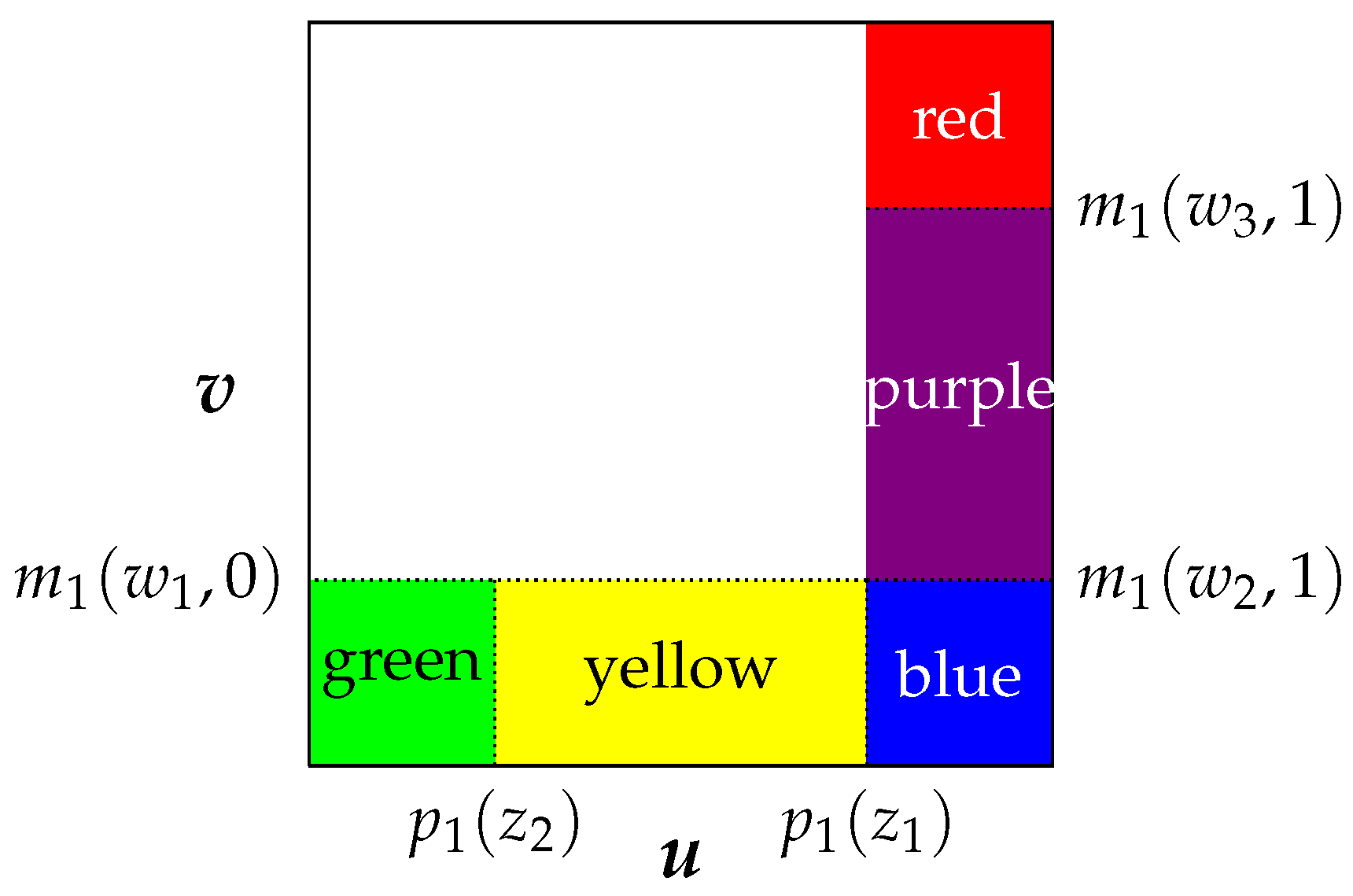
Example 1. Consider Figure 1 and suppose for now that the $m_s$ functions are identified and that the joint support of the covariates equals the product of their marginal supports. Let $x_1,x_2,w_1,w_2,w_3,z_1,z_2$ be values in their respective supports (i.e., ${\mathcal{S}}_X,{\mathcal{S}}_W,{\mathcal{S}}_Z$), such that $m_1(w_1,0)=m_1(w_2,1)<m_1(w_3,1)$ and $0<p_1(z_2)<p_1(z_1)<1$, as is depicted in Figure 1. Then, the following quantities are identified directly from the data.

$$\left\{\begin{array}{cc}\hfill \delta (x^{*},0,0,w_1,z_2)& =\kappa (\text{green},\alpha (x^{*},0,0)),\hfill \\ \hfill \delta (x^{*},0,0,w_1,z_1)& =\kappa (\text{green+yellow},\alpha (x^{*},0,0)),\hfill \\ \hfill \delta (x_1,0,1,w_2,z_1)& =\kappa (\text{blue},\alpha (x_1,0,1)),\hfill \\ \hfill \delta (x_1,0,1,w_2,z_2)& =\kappa (\text{blue+yellow},\alpha (x_1,0,1)),\hfill \\ \hfill \delta (x_1,0,1,w_3,z_1)& =\kappa (\text{blue+purple},\alpha (x_1,0,1)),\hfill \\ \hfill \delta (x_2,1,1,w_3,z_1)& =\kappa (\text{red},\alpha (x_2,1,1)),\hfill \\ \hfill \delta (x_2,1,1,w_2,z_1)& =\kappa (\text{red+purple},\alpha (x_2,1,1)),\hfill \\ \hfill \delta (x_3,1,0,w_1,z_1)& =\kappa (\text{blank},\alpha (x_3,1,0)).\hfill \end{array}\right.$$

(18)

Subtracting the first and third lines in (18) from the second and fourth lines, respectively, yields $\kappa (\text{yellow},\alpha (x^{*},0,0))$ and $\kappa (\text{yellow},\alpha (x_1,0,1))$, which are equal if and only if $\alpha (x^{*},0,0)=\alpha (x_1,0,1)$. Likewise, subtracting the third and sixth lines in (18) from the fifth and seventh lines allows one to verify whether $\alpha (x_1,0,1)=\alpha (x_2,1,1)$. We can verify that $\alpha (x_1,1,1)=\alpha (x_2,1,0)$ analogously.

Figure 1. Simple matching procedures.

Figure 1. Simple matching procedures.

Once values $x_1,x_2,x_3$ are found, such that $\alpha (x^{*},0,0)=\alpha (x_1,0,1)=\alpha (x_2,1,1)=\alpha (x_3,1,0)$, $\kappa ({\mathcal{S}}_{uv},\alpha (x^{*},0,0))$ can be computed as (for instance) the sum of $\delta (x^{*},0,0,w_1,z_1)$, $\delta (x_1,0,1,w_2,z_1)$, $\delta (x_2,1,1,w_2,z_1)$ and $\delta (x_3,1,0,w_1,z_1)$.  ☐

Finally, we note that there exists an alternative, but not particularly attractive, possibility: identification-at-infinity. From (15), it should be apparent that if we can find a sequence $\{(z_n,w_n)\}$, such that

$$\underset{n\to \infty }{lim}{p}_1(z_n)=1,\underset{n\to \infty }{lim}{m}_1(w_n,0)=1,$$

then identification of $\psi (x^{*},0,0)$ obtains, since

$$\underset{n\to \infty }{lim}\mathbb{E}\left[y(s=0)(d=0)|x=x^{*},w=w_n,z=z_n\right]=\mathbb{E}\left[g\left(\alpha (x^{*},0,0),ϵ\right\}\{(u,v)\in {\mathcal{U}}^2)\right]=\psi (x^{*},0,0).$$

However, such an identification-at-infinity argument is undesirable since it generally makes inefficient use of the data [27] and imposes extreme support restrictions. Therefore, we do not consider this possibility.

In the remainder of this paper, more general versions of the procedures sketched above are formally expressed in terms of a Dynkin system, and their power is illustrated using some concrete examples.

4. Identification of m

We now establish the identification of $m_{s^{*}}(w^{*},d^{*})$ formally. Define8

$$\theta (V,m)=\mathbb{P}(u\in V,v\le m),V\subset \mathcal{U},m\in \mathcal{U}.$$

Further, let ${\mathcal{S}}_z(w)$ be the support of $z$ conditional on $w=w$ and define

$$\mathcal{V}(d,w)=\left\{(p_d(z),p_{d+1}(z)]:z\in {\mathcal{S}}_z(w)\right\},d=0,\dots ,{\eta }_d.$$

(19)

Then, $\theta (V,m_s(w,d))$ is identified when $V\in \mathcal{V}(d,w)$ because

$$\theta \left((p_d(z),p_{d+1}(z)],m_s(w,d)\right)=\mathbb{P}(s<s,d=d|w=w,z=z).$$

(20)

We now show that $\theta (V,m_s(w,d))$ is identified for a much broader class of sets than $\mathcal{V}(d,w)$.

Definition 1. ${\mathcal{D}}^{*}(d,s,w)$ is the collection ${\mathcal{D}}_{\infty }^{*}(d,s,w)$ in the following iterative scheme. Let ${\mathcal{D}}_0^{*}(d,s,w)=\mathcal{V}(d,w)$. Then, for all $t\ge 0$, ${\mathcal{D}}_{t+1}^{*}(d,s,w)$ consists of all sets $A^{*}$, such that at least one of the following conditions is satisfied, where μ denotes the standard Lebesgue measure over $\mathcal{U}$.

(i)

$A^{*}\in {\mathcal{D}}_t^{*}(d,s,w)$;

(ii)

$\exists A_1,A_2\in {\mathcal{D}}_t^{*}(d,s,w):A_1\subset A_2,\mu (A_2-A_1)>0,A^{*}=A_2-A_1$;

(iii)

$\exists A_1,A_2\in {\mathcal{D}}_t^{*}(d,s,w):A_1\cap A_2=\varnothing ,\mu (A_1\cup A_2)>0,A^{*}=A_1\cup A_2$;

(iv)

$\exists (\overline{d},\overline{s},\overline{w}):m_s(d,w)=m_{\overline{s}}(\overline{d},\overline{w}),{\mathcal{D}}_t^{*}(d,s,w)\cap {\mathcal{D}}_t^{*}(\overline{d},\overline{s},\overline{w})\ne \varnothing ,A^{*}\in {\mathcal{D}}_t^{*}(\overline{d},\overline{s},\overline{w})$.  ☐

The conditions in Definition 1 are similar to those in [3]. Note that ${\mathcal{D}}^{*}(d,s,w)$ depends on s because of Condition (iv). The importance of Condition (iv) will become apparent in Lemma 1 below. The main difference between [3] and what we have here for the identification of m is that the collection in Definition 1 now also has an argument s: identification of ψ is substantially more involved than that.

Note that $\{{\mathcal{D}}_t^{*}(d,s,w):t=0,1,\dots \}$ is an increasing sequence of collections, such that ${\mathcal{D}}^{*}(d,s,w)$ is the infinite union of ${\mathcal{D}}_t^{*}(d,s,w)$’s.9 Note further that ${\mathcal{D}}^{*}(d,s,w)$ is indexed by $s,w$, as well as d. If ${\mathcal{S}}_z(w)$ is the same for all w values, then the argument pursued in this section is simpler, but such support restrictions are undesirable, because they exclude the possibility that $w,z$ have elements in common, and they also preclude the situation in which certain combinations of $(w,z)$ values cannot occur.

All elements of ${\mathcal{D}}^{*}$ are defined in terms of (combinations of) the unknown $p_d$ and $m_s$ functions. Hence, each element can be thought of as an unknown parameter. In Lemma 1, we show that all elements in ${\mathcal{D}}^{*}$ are identified. Subsequently, we obtain a condition that is sufficient for identification of $m_{s^{*}}(w^{*},d^{*})$.

Lemma 1. Suppose that Assumptions A and B are satisfied.

(i) 

For all $(d,s,w)\in {\mathcal{S}}_{dsw}$, every $V\in {\mathcal{D}}^{*}(d,s,w)$ is identified;

(ii) 

$\theta (V,m_s(w,d))$ is identified whenever $(d,s,w)\in {\mathcal{S}}_{dsw}$ and $V\in {\mathcal{D}}^{*}(d,s,w)$.

Proof. See Appendix A.  ☐

Assumption E. $\mathcal{U}\in {\mathcal{D}}^{*}(d^{*},s^{*},w^{*})$.

Since $\{{\mathcal{D}}_t^{*}(d^{*},s^{*},w^{*}):t=0,1,2,\dots \}$ is an increasing sequence of collections of sets and $d,s$ take finitely many values, Assumption E is satisfied when there exists a finite T, such that $\mathcal{U}\in {\mathcal{D}}_T^{*}(d^{*},s^{*},w^{*})$. Assumption E is testable, because for any finite t, all elements of ${\mathcal{D}}_t^{*}(d,s,w)$ are identified.

Theorem 1. If Assumptions A, B and E are satisfied then, $m_{s^{*}}(w^{*},d^{*})$ is identified.

Proof. See Appendix A.  ☐

Assumption E involves conditions on the support of $z$; the class ${\mathcal{D}}^{*}(d,s,w)$ is mostly determined by the amount of variation available in $z$ given $d=d,s<s,w=w$. For example, consider the simple case ${\eta }_d=1$. Suppose that there exist $s,\overline{s},w,\overline{w}$, such that $m_s(w,0)=m_{\overline{s}}(\overline{w},1)$. Then, Assumption E is satisfied if the support of $z$ contains values $z,\overline{z}$ with $p_1(z)<p_1(\overline{z})$. Please note that even though $\mathcal{V}(0,w)=\left\{(0,p_1(z)],(0,p_1(\overline{z})]\right\}$ does not contain a partition of $\mathcal{U}$, we have ${\mathcal{D}}_1^{*}(0,s,w)\cap {\mathcal{D}}_1^{*}(1,\overline{s},\overline{w})=\left\{(p_1(z),p_1(\overline{z})]\right\}$, and therefore, the matching mechanism (iv) in Definition 1 implies that ${\mathcal{D}}^{*}(0,s,w)$ contains a partition of $\mathcal{U}$.

Indeed, suppose that ${\mathcal{D}}^{*}(d^{*},s^{*},w^{*})\cap {\mathcal{D}}^{*}(\overline{d},\overline{s},\overline{w})\ne \varnothing$ for some $(\overline{d},\overline{s},\overline{w})\in {\mathcal{S}}_{dsw}$. Then, by (iv) in Definition 1, $m_{s^{*}}(w^{*},d^{*})=m_{\overline{s}}(\overline{w},\overline{d})$ implies that ${\mathcal{D}}^{*}(d^{*},s^{*},w^{*})={\mathcal{D}}^{*}(\overline{d},\overline{s},\overline{w})$. Therefore, not only $\mathcal{V}(d^{*},w^{*})$, but also $\mathcal{V}(\overline{d},\overline{w})$ should be taken into account, which is particularly useful when $d^{*}\ne \overline{d}$. This reasoning suggests a simple sufficient condition, which we state as a corollary.

Corollary 1 (Sufficient conditions). Suppose that Assumptions A and B are satisfied and that ${\mathcal{S}}_{wz}={\mathcal{S}}_w\times {\mathcal{S}}_z$. Suppose further that there exists a sequence $\{(s_j,w_j)\in {\mathcal{S}}_{sw}:j=0,1,\dots ,{\eta }_d\}$, such that $m_{s_j}(w_j,j)=m_{s^{*}}(w^{*},d^{*})$ for all $j=0,1,\dots ,{\eta }_d$. Further, suppose that:

$$\forall j=1,\dots ,{\eta }_d-1:\underset{z\in {\mathcal{S}}_z}{inf}{p}_{j+1}(z)<\underset{z\in {\mathcal{S}}_z}{sup}{p}_j(z),$$

(21)

where each $p_j$ is a continuous function and $z$ is continuously distributed. Then, $m_{s^{*}}(w^{*},d^{*})$ is identified.

Please note that Corollary 1 imposes restrictions on the relationship between $p_j$ and $p_{j+1}$ (for all values of j), but it does not require there to be a direct relationship between $p_j$ and $p_{j+2}$. Indeed, the matching procedure can be chained in the sense that we can first establish equality of $m_{s_0}(w_0,0)$ to $m_{s_1}(w_1,1)$, then uncover that $m_{s_0}(w_0,0)=m_{s_1}(w_1,1)=m_{s_2}(w_2,2)$, and so on.

To illustrate Corollary 1, consider the following example.

Example 2 (Ordered response). Suppose that for all $d,z$ and some ${\beta }_0$ and $-\infty ={\gamma }_0<{\gamma }_1<\dots <{\gamma }_{{\eta }_d+1}=\infty$, $p_d(z)=\Phi ({\gamma }_d+{\beta }^{\top }z)$, as would be the case in an ordered probit model. This is one of the least favorable cases for our procedure, since for all $z,z^{*}$ and $d=1,\dots ,{\eta }_d$, $p_d(z)<p_d(z^{*})\Rightarrow p_{d+1}(z)\le p_{d+1}(z^{*})\text{and}{p}_{d-1}(z)\le p_{d-1}(z^{*})$.

Therefore, condition (21) in Corollary 1 is satisfied if

$$\underset{z,z^{*}\in {\mathcal{S}}_z}{sup}{\beta }^{\top }(z-z^{*})\ge \underset{d=1,\dots ,{\eta }_d-1}{max}({\gamma }_{d+1}-{\gamma }_d).\hspace{1em}☐$$

To illustrate the idea of Theorem 1, we provide the following two fairly concrete examples. Let

$$\begin{array}{cc}\hfill {\pi }_{sd}(w,z)=\mathbb{P}(s<s,d=d|w=w,z=z)=\mathbb{P}\{p_d(z)<& u\le p_{d+1}(z),v\le m_s(w,d)\}\hfill \\ & =\theta (p_d(z)p_{d+1}(z),m_s(w,d)),\hfill \end{array}$$

(22)

which is identified provided that $z\in {\mathcal{S}}_z(w)$.

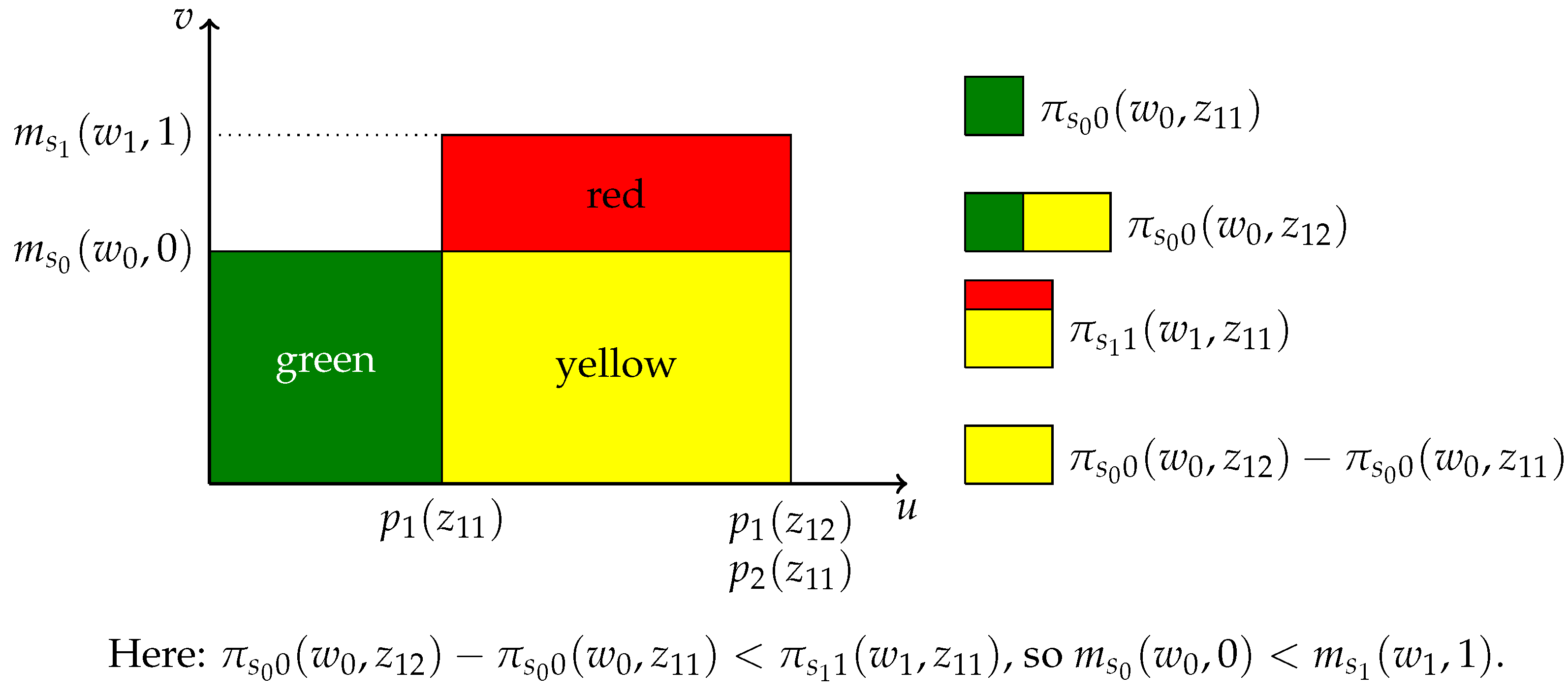
Example 3 (Uncovering that $m_{s_0}(w_0,0)=m_{s_1}(w_1,1)$). We verify whether $m_{s_0}(w_0,0)=m_{s_1}(w_1,1)$ for some candidate pair $(s_1,w_1)$. Our approach is described below and illustrated in Figure 2, which assumes the existence of values $z_{11},z_{12}$, such that $p_1(z_{12})=p_2(z_{11})$. It should be apparent from Figure 2 that $m_{s_0}(w_0,0)=m_{s_1}(w_1,1)$ if and only if the measure of the red area is zero.

Figure 2. Verifying whether $m_{s_0}(w_0,0)=m_{s_1}(w_1,1)$.

Figure 2. Verifying whether $m_{s_0}(w_0,0)=m_{s_1}(w_1,1)$.

The measures of the yellow area, the yellow plus the green area and the yellow plus the red area are identified directly from the data. The measure of the yellow area can then be learned as $(\text{yellow+green})-\text{green}$, and finally, the measure of the red area as $(\text{yellow+red})-\text{yellow}$.

The formal identification argument is as follows. First,

$${\mathcal{D}}_0^{*}(0,s_0,w_0)\supset \{0,p_1(z_{11}),0,p_1(z_{12})\},{\mathcal{D}}_0^{*}(1,s_1,w_1)\supset \{p_1(z_{11})p_2(z_{11})\}.$$

Using (i) and (ii) of Definition 1, it follows that $V=p_1(z_{11})p_1(z_{12})=p_1(z_{11})p_2(z_{11})\in {\mathcal{D}}_1^{*}(0,s_0,w_0)\cap {\mathcal{D}}_1^{*}(1,s_1,w_1)$. Thus,

$$\left\{\begin{array}{cc}\hfill \theta \left(V,m_{s_0}(w_0,0)\right)& ={\pi }_{s_{0}0}(w_0,z_{12})-{\pi }_{s_{0}0}(w_0,z_{11}),\hfill \\ \hfill \theta \left(V,m_{s_1}(w_1,d_1)\right)& ={\pi }_{s_{1}1}(w_1,z_{11}),\hfill \end{array}\right.$$

are both identified; they are equal if and only if $m_{s_1}(w_1,1)=m_{s_0}(w_0,0)$.  ☐

In Example 3 it is implicitly assumed that $z_{11},z_{12}\in {\mathcal{S}}_z(w_0)$ and that $z_{11}\in {\mathcal{S}}_z(w_1)$. However, Theorem 1 does not require this. Indeed, if there exist $z_{110},z_{111}$, such that $p_1(z_{110})=p_1(z_{111})$, $p_1(z_{12})=p_2(z_{111})$ and both $z_{110},z_{12}\in {\mathcal{S}}_z(w_0)$ and $z_{111}\in {\mathcal{S}}_z(w_1)$, then we can match ${\pi }_{s_{0}0}(w_0,z_{12})-{\pi }_{s_{0}0}(w_0,z_{110})$ with ${\pi }_{s_{1}1}(w_1,z_{111})$ to obtain $m_{s_0}(w_0,0)=m_{s_1}(w_1,1)$.

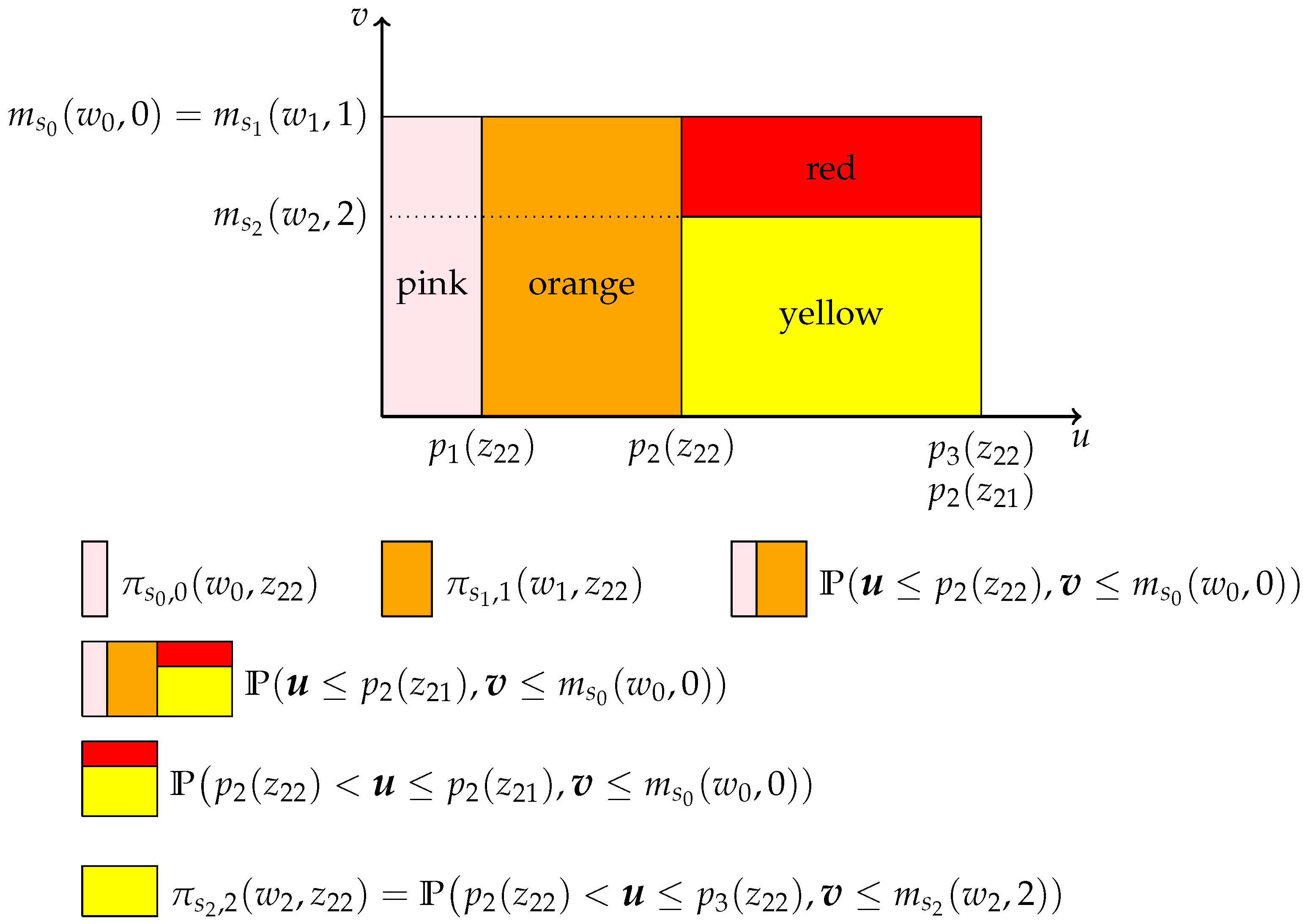
Example 4 (Verifying that $m_{s_1}(w_1,1)=m_{s_2}(w_2,2)$). We now turn to the task of verifying that $m_{s_1}(w_1,1)=m_{s_2}(w_2,2)$ once $m_{s_0}(w_0,0)=m_{s_1}(w_1,1)$ has been established. The procedure is illustrated in Figure 3 and described below, which presumes the existence of $z_{21},z_{22}$ for which $p_3(z_{22})=p_2(z_{21})$.

Again, the question is whether the measure of the red area equals zero. Pink, orange and yellow are directly identified, which allows us to deduce $(\text{pink}+\text{orange})$. Further, $(\text{pink}+\text{orange}+\text{yellow}+\text{red})={\pi }_{s_{0}0}(w_0,z_{21})+{\pi }_{s_{1}1}(w_1,z_{21})$ is identified, and hence, so is $(\text{yellow}+\text{red})$, which in turn implies the identification of red.

Figure 3. Verifying whether $m_{s_1}(w_1,1)=m_{s_2}(w_2,2)$ given that $m_{s_0}(w_0,0)=m_{s_1}(w_1,1)$.

Figure 3. Verifying whether $m_{s_1}(w_1,1)=m_{s_2}(w_2,2)$ given that $m_{s_0}(w_0,0)=m_{s_1}(w_1,1)$.

Formally, it follows from Example 3 that ${\mathcal{D}}_t^{*}(0,s_0,w_0)={\mathcal{D}}_t^{*}(1,s_1,w_1)$ for all $t\ge 2$. Therefore, for sufficiently large t, $V=p_2(z_{22})p_2(z_{21})\in {\mathcal{D}}_t^{*}(0,s_0,w_0)$. However, since $V=p_2(z_{22})p_3(z_{22})\in {\mathcal{D}}_2^{*}(0,s_2,w_2)$, the equality of $m_{s_0}(w_0,0)$ and $m_{s_2}(w_2,2)$ can be verified using the set V.  ☐

Once we have ascertained that $m_{s_0}(w_0,0)=m_{s_1}(w_1,1)=m_{s_2}(w_2,2)$, we can identify

$$\begin{array}{cc}\hfill \theta (0p_3(z_{22}),& m_{s_0}(w_0,0))=\hfill \\ & \theta (0p_1(z_{22}),m_{s_0}(w_0,0))+\theta (p_1(z_{22})p_2(z_{22}),m_{s_1}(w_1,1))+\theta (p_2(z_{22})p_3(z_{22}),m_{s_2}(w_2,2)),\hfill \end{array}$$

since $(0,p_3(z_{22})]=(0,p_1(z_{22})]\cup (p_1(z_{22}),p_2(z_{22})]\cup (p_2(z_{22}),p_3(z_{22})]$.

When the support of $z$ and $w$ is the Cartesian product of the marginals (as in these examples), Assumption E is reduced to the requirement that $p_d$ has sufficient variability and $z$ sufficiently rich support, as in Corollary 1.

5. Identification of ψ

We now turn to the identification of the main object of interest, i.e., ${\psi }^{*}=\psi (x^{*},s^{*},d^{*})$, for which we use the fact that the m function is identified.

Recall from (14) that for $A\subset {\mathcal{S}}_{uv}$,

$$\kappa (A,a)=\mathbb{E}[g(a,ϵ)\{(u,v)\in A\}].$$

The role of κ is similar to that of the function θ in Section 4. Indeed, if A is a set of positive measure, then by Assumption C, $\kappa (A,a)=\kappa (A,\tilde{a})$ if and only if $a=\tilde{a}$. We start with the identification of κ.

Let ${\mathcal{S}}_{wz}(x)$ be the support of $(w,z)$ conditional on $x=x$. We define $\mathcal{M}$ to be the collection of $(d,s,w)$ triples for which $m_s(w,d)$ and $m_{s+1}(w,d)$ are both identified. Formally, we let

$${\mathcal{M}}^{*}(s)=\left\{\begin{array}{cc}\left\{(d,w):\mathcal{U}\in {\mathcal{D}}^{*}(d,1,w)\right\},\hfill & s=0,\hfill \\ \left\{(d,w):\mathcal{U}\in {\mathcal{D}}^{*}(d,s,w)\cap {\mathcal{D}}^{*}(d,s+1,w)\right\},\hfill & 1\le s\le {\eta }_s-1,\hfill \\ \left\{(d,w):\mathcal{U}\in {\mathcal{D}}^{*}(d,{\eta }_s,w)\right\},\hfill & s={\eta }_s,\hfill \end{array}\right.$$

$$\mathcal{M}=\left\{(d,s,w):(d,w)\in {\mathcal{M}}^{*}(s)\right\},$$

and

$$\mathcal{K}(x,s,d)=\left\{\left(p_d(z),p_{d+1}(z)\right]\times \left(m_s(w,d),m_{s+1}(w,d)\right]:(w,z)\in {\mathcal{S}}_{wz}(x)\text{and}(d,s,w)\in \mathcal{M}\right\}.$$

10

Therefore, by Theorem 1 $\mathcal{K}(x,s,d)$ is a collection of nonempty rectangles whose corner points are all identified under Assumptions A and B. Moreover, for $K=p_d(z)p_{d+1}(z)\times m_s(w,d)m_{s+1}(w,d)$, $\kappa (K,\alpha (x,s,d))$ is identified, because

$$\kappa (K,\alpha (x,s,d))=\mathbb{E}[y(d=d)(s=s)|x=x,w=w,z=z].$$

(23)

We now extend $\mathcal{K}(x,s,d)$ to a larger class of sets K for which the identification of $\kappa (K,\alpha (x,s,d))$ obtains.

Definition 2. $\mathcal{D}(x,s,d)$ is the collection ${\mathcal{D}}_{\infty }(x,s,d)$ in the following iterative scheme. Let ${\mathcal{D}}_0(x,s,d)=\mathcal{K}(x,s,d)$. Then, for all $t\ge 0$, ${\mathcal{D}}_{t+1}(x,s,d)$ consists of all sets $A^{*}$, such that at least one of the following four conditions is satisfied, where ${\mu }^{*}$ denotes the standard Lebesgue measure over ${\mathcal{U}}^2$.

(i)

$A^{*}\in {\mathcal{D}}_t(x,s,d)$;

(ii)

$\exists A_1,A_2\in {\mathcal{D}}_t(x,s,d):A_1\subset A_2,{\mu }^{*}(A_2-A_1)>0,A^{*}=A_2-A_1$;

(iii)

$\exists A_1,A_2\in {\mathcal{D}}_t(x,s,d):A_1\cap A_2=\varnothing ,{\mu }^{*}(A_1\cup A_2)>0,A^{*}=A_1\cup A_2$;

(iv)

$\exists (\tilde{x},\tilde{s},\tilde{d}):\alpha (\tilde{x},\tilde{s},\tilde{d})=\alpha (x,s,d),{\mathcal{D}}_t(x,s,d)\cap {\mathcal{D}}_t(\tilde{x},\tilde{s},\tilde{d})\ne \varnothing ,A^{*}\in {\mathcal{D}}_t(\tilde{x},\tilde{s},\tilde{d})$.  ☐

The collection $\mathcal{D}(x,s,d)$ (like ${\mathcal{D}}^{*}(d,s,w)$) consists of sets defined in terms of the unknown $p_d,m_s,\alpha$ functions, such that $\mathcal{D}(x,s,d)$ can be interpreted as a set of unknown parameters.

Lemma 2. Suppose that Assumptions A to C and E are satisfied.

(i) 

For all $(x^{*},s^{*},d^{*})\in {\mathcal{S}}_{xsd}$, every $K\in \mathcal{D}(x^{*},s^{*},d^{*})$ is identified;

(ii) 

$\kappa (K,\alpha (x^{*},s^{*},d^{*}))$ is identified whenever $(x,s,d)\in {\mathcal{S}}_{xsd}$ and $K\in \mathcal{D}(x^{*},s^{*},d^{*})$.

Assumption F. ${\mathcal{U}}^2\in \mathcal{D}(x^{*},d^{*},s^{*})$.

Like for Assumption E, Assumption F equivalently requires that there be a finite T, such that ${\mathcal{U}}^2\in {\mathcal{D}}_T(x^{*},d^{*},s^{*})$.

Theorem 2. Suppose that Assumptions A to C and F are satisfied. Then, ${\psi }^{*}$ is identified.

Our method for identifying ψ is similar to our method for identifying m described in Section 4: $\mathcal{D}(x,s,d)$ is now generated from a collection of rectangles, not a collection of intervals. Further, if we can ascertain that $\alpha (x^{*},s^{*},d^{*})=\alpha (\overline{x},\overline{s},\overline{d})$, then $\mathcal{D}(x^{*},s^{*},d^{*})\cap \mathcal{D}(\overline{x},\overline{s},\overline{d})\ne \varnothing$ implies that the two collections in fact coincide. This is particularly helpful when $s^{*}\ne s$ and $d^{*}\ne \overline{d}$.

We now state a set of sufficient conditions for the identification of ${\psi }^{*}$.

Corollary 2 (Sufficient conditions). Suppose that there exists a sequence $\left\{x_{ij}\in {\mathcal{S}}_x:i=0,1,\cdots ,{\eta }_s,j=0,1,\cdots ,{\eta }_d\right\}$, such that $\alpha (x_{ij},i,j)=\alpha (x^{*},s^{*},d^{*})$ for all $i,j$. Further, suppose that ${\mathcal{S}}_{xwz}={\mathcal{S}}_x\times {\mathcal{S}}_w\times {\mathcal{S}}_z$. If $w,z$ are continuously distributed and that for some continuous functions $m_1,\dots ,m_{{\eta }_s},p_1,\dots ,p_{{\eta }_d}$,

(i) 

for $i=1,\dots ,{\eta }_s-1$ and $j=0,1,\dots ,{\eta }_d$

$$\underset{w\in {\mathcal{S}}_w}{inf}{m}_{i+1}(w,j)<\underset{w\in {\mathcal{S}}_w}{sup}{m}_i(w,j),$$

(ii) 

for $i=1,2,\dots ,{\eta }_s$ and $j=1,\dots ,{\eta }_d-1$,

$$\underset{w\in {\mathcal{S}}_w}{inf}{m}_i(w,j+1)<\underset{w\in {\mathcal{S}}_w}{sup}{m}_i(w,j),\underset{z\in {\mathcal{S}}_z}{inf}{p}_{j+1}(z)<\underset{z\in {\mathcal{S}}_z}{sup}{p}_j(z).$$

Then, ${\psi }^{*}$ is identified.

Corollary 2 is a two-dimensional analog to Corollary 1.

We now consider a simple example that illustrates the basics of the machinery developed above. The example is limited relative to the theoretical results in several respects, which we discuss after the example.

Example 5. We will focus on the simplest interesting case, i.e., ${\eta }_s={\eta }_d=2$ with covariate support ${\mathcal{S}}_{xwz}={\mathcal{S}}_x\times {\mathcal{S}}_w\times {\mathcal{S}}_z$. Because of the absence of support restrictions, we will use $\mathcal{K}(s,d)$ instead of $\mathcal{K}(x,s,d)$ in this example. Identification of $p_d$ is trivial, and identification of $m_s$ was discussed in Section 4, so the discussion below starts from the point at which identification of $p_d$ and $m_s$ has already been established.

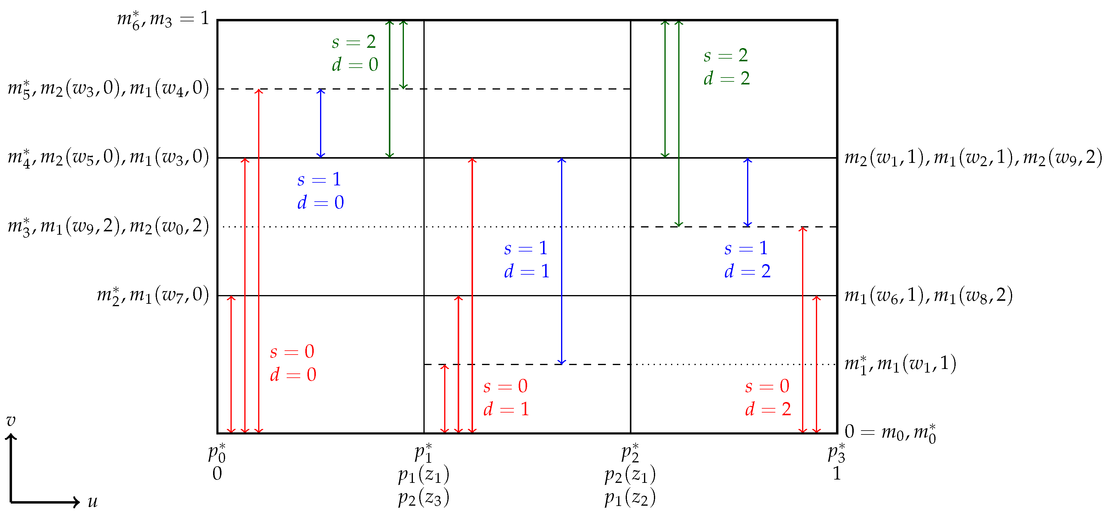
The example is illustrated in Figure 4, which depicts a situation in which ${\psi }^{*}$ is identified for all values of $x^{*},s^{*},d^{*}$ provided that $\alpha (x,s^{*},d^{*})$ varies sufficiently as a function of x. In the discussion below, we assume that there exists a $\{x_{sd}\}$, such that $\alpha (x_{sd},s,d)$ is the same for all values of s and d, such that the existence of the $w,z$ combinations in Figure 4 is sufficient. We show that for such $\{x_{sd}\}$, $\mathcal{D}(x_{sd},s,d)$ is the same for all values of $s,d$, which implies that ${\mathcal{U}}^2$ is an element of $\mathcal{D}(x_{sd},s,d)$ for all $s,d$, which implies identification. From hereon, we use the shorthand notation $\mathcal{D}(s,d)$ to mean $\mathcal{D}(x_{sd},s,d)$.

Figure 4. Identification of ψ if ${\eta }_s={\eta }_d=2$.

Figure 4. Identification of ψ if ${\eta }_s={\eta }_d=2$.

We start by showing that $\mathcal{D}(1,1)=\mathcal{D}(0,1)$ if $\alpha (x_{11},1,1)=\alpha (x_{01},0,1)$. Let

$$K_{hrij}=p_h^{*}{p}_r^{*}\times m_i^{*}{m}_j^{*},h=0,1;r=h+1,\dots ,2;i=0,\dots ,5;j=i+1,\dots ,6.$$

Since $p_1(z_1)=p_1^{*}$, $p_2(z_1)=p_2^{*}$, $m_1(w_1,1)=m_1^{*}$ and $m_2(w_1,1)=m_4^{*}$, it follows that $K_{1214}\in \mathcal{D}(1,1)$. Likewise, using $m_1(w_1,1)=m_1^{*}$ and $m_1(w_2,1)=m_4^{*}$, it follows that $K_{1201},K_{1204}\in \mathcal{D}(0,1)$, which implies that $K_{1214}=K_{1204}\cap K_{1201}\in \mathcal{D}(0,1)$, also. Therefore, $K_{1214}\in \mathcal{D}(1,1)\cap \mathcal{D}(0,1)$, such that by the assumption on α made earlier in the example and Condition (iv) of Definition 2, $\mathcal{D}(1,1)=\mathcal{D}(0,1)$.

We next show that $\mathcal{D}(0,0)=\mathcal{D}(1,0)=\mathcal{D}(2,0)$. Now, $K_{0145}\in \mathcal{D}(1,0)$, because $m_1(w_3,0)=m_4^{*}<m_5^{*}=m_2(w_3,0)$. Further, $m_1(w_3,0)=m_4^{*}<m_5^{*}=m_1(w_4,0)$ implies that $K_{0104},K_{0105}\in \mathcal{D}(0,0)$ and, hence, that $K_{0145}=K_{0105}\cap K_{0104}\in \mathcal{D}(0,0)$. Likewise, $m_2(w_5,0)=m_4^{*}<m_5^{*}=m_2(w_3,0)$, such that $K_{0145}=K_{0146}-K_{0156}\in \mathcal{D}(2,0)$. Consequently, $K_{0145}\in \mathcal{D}(0,0)\cap \mathcal{D}(1,0)\cap \mathcal{D}(2,0)$, which (together with the assumption on α used in this example) implies that $\mathcal{D}(0,0)=\mathcal{D}(1,0)=\mathcal{D}(2,0)$.

Given that $m_1(w_6,1)=m_2^{*}$, it follows that $K_{1202}\in \mathcal{D}(0,1)$. Likewise, using $w_7$, $K_{0102},K_{0202}\in \mathcal{D}(0,0)$, and hence, $K_{1202}=K_{0102}\cap K_{0202}\in \mathcal{D}(0,0)$, also. Repeating the same argument for $w_8$ results in $\mathcal{D}(0,0)\cap \mathcal{D}(0,1)\cap \mathcal{D}(0,2)\ne \varnothing$, and hence, $\mathcal{D}(0,0)=\mathcal{D}(0,1)=\mathcal{D}(0,2)=\mathcal{D}(1,0)=\mathcal{D}(1,1)=\mathcal{D}(2,0)$.

Finally, using $w_9,w_0$, it follows that $K_{2334}\in \mathcal{D}(1,2)\cap \mathcal{D}(2,2)$, and using $w_8,w_9$, it can be deduced that $K_{1224}\in \mathcal{D}(1,1)\cap \mathcal{D}(1,2)$, such that $\mathcal{D}(s,d)$ is identical for all $s,d$.

To see that ${\mathcal{U}}^2\in \mathcal{D}(1,1)$, note that each of the nine rectangles with solid boundaries in Figure 4 belongs trivially to some $\mathcal{D}(s,d)$ (e.g., $K_{1224}\in \mathcal{D}(1,1)$). Since the union of the nine rectangles is exactly ${\mathcal{U}}^2$ and $\mathcal{D}(s,d)$ is the same for all $s,d$, identification is hereby established.  ☐

In the above example, it was shown that $\mathcal{D}(s,d)$ was the same for all values of $s,d$. This is not necessary for the identification of ${\psi }^{*}$. Indeed, all that is required is that ${\mathcal{U}}^2\in \mathcal{D}(x^{*},s^{*},d^{*})$; it does not matter which combinations of $(s,d)$ pairs are matched with each other, as long as the Dynkin system generated by the union of their $\mathcal{K}$-sets includes ${\mathcal{U}}^2$ as an element.

Example 5 is limited in several respects. First, the support of covariates was assumed to be the Cartesian product of the marginal supports and to be independent of $s,d$. With support restrictions, the procedure to establish identification of ${\psi }^{*}$ would be similar, but more care should be taken in the selection of $w,z$ pairs to ensure that the support restrictions are satisfied. For instance, Figure 4 of Example 5 indicates that $(w_j,z_1)$ belongs to ${\mathcal{S}}_{wz}$ for a number of different values of j, but this condition can be relaxed in numerous ways.

Further, it was assumed that ${\eta }_s={\eta }_d=2$. With more than two categories, the essence of the identification procedure does not change, but Figure 4 would be messier. An essential ingredient of Example 5 is that there are values of $z_1,z_3$ for which $p_1(z_1)=p_2(z_3)$ and likewise for $m_s$. This is analogous to Corollary 1. It should be pointed out that with more than three categories (${\eta }_d>2$ or ${\eta }_s>2$), it is not necessary for there to be a $z_4$-value for which $p_1(z_1)=p_3(z_4)$. Indeed, what is needed is for there to be a pair $z_4,z_5$, such that $p_2(z_4)=p_3(z_5)$. As mentioned earlier, such a chaining argument can be extended to any number of categories, i.e., one could obtain a set of sufficient conditions similar to those in Corollary 1.

6. Decomposing the Effect of $d$

As mentioned in Section 2, it is possible to use the methodology developed in this paper to identify objects that are not based on ψ. In this section, we show that the average total effect and its decomposition in (6) is indeed identified by the same method. For this purpose, we will explain how to use the matches of the m and α functions, because we have already explained in detail how to achieve those matches and how Dynkin systems can help.

We focus on the special case with binary $s,d$; the general case is similar. We discuss the identification of

$${\psi }^{\circ }(x,w,d,\tilde{d})=\mathbb{E}g\left(\alpha (x,s_d(w),\tilde{d}),ϵ\right),$$

where $s_d(w)$ is the counterfactual value of $s$ when $d$ is fixed at d given $w=w$, i.e., $s_d=\{v>m_1(w,d)\}$. Therefore, (6) is now

$$\begin{array}{cc}\underset{\text{Average}\text{Total}\text{Effect}\text{of}d}{\underbrace{{\psi }^{\circ }(x,w,1,1)-{\psi }^{\circ }(x,w,0,0)}}\hfill & \\ & \hfill =\underset{\text{Direct}\text{Effect}\text{of}d}{\underbrace{{\psi }^{\circ }(x,w,1,1)-{\psi }^{\circ }(x,w,1,0)}}+\underset{\text{Indirect}\text{Effect}\text{of}d}{\underbrace{{\psi }^{\circ }(x,w,1,0)-{\psi }^{\circ }(x,w,0,0)}}.\end{array}$$

(24)

We note that ${\psi }^{\circ }$ and ψ are different objects unless $v$ and $ϵ$ are known to be independent11. However, the identification of ${\psi }^{\circ }$ can also be achieved using our matching procedure.

We focus on ${\psi }^{\circ }(x,w,0,0)$; the other cases are similar. We have

$${\psi }^{\circ }(x,w,0,0)=\mathbb{E}\left[\{d=0\}g\left(\alpha (x,s_0(w),0),ϵ\right)\right]+\mathbb{E}\left[\{d=1\}g\left(\alpha (x,s_0(w),0),ϵ\right)\right].$$

The first term on the right-hand side can be identified by using $\mathbb{E}\left[\{d=0\}y|x=x,w=w,z\right]$. For the second term on the right-hand side, consider $\mathbb{E}\left[(d=1)g\left(\alpha (x,s_0(w),0),ϵ\right)|x=x,w=w,z=z\right],$ which can be written as

$$\begin{array}{cc}\hfill \mathbb{E}[\{u>p_1(z)\}\{v\le m_1(w,0)\}g\left(\alpha (x,0,0),ϵ\right)& ]+\hfill \\ & \mathbb{E}\left[\{u>p_1(z)\}\{v>m_1(w,0)\}g\left(\alpha (x,1,0),ϵ\right)\right].\hfill \end{array}$$

(25)

The method developed in the paper explains how to find $(x,w)$ and $(\tilde{w},\tilde{x})$, such that $\alpha (x,1,0)=\alpha (\tilde{x},1,1)$ and $m_1(w,0)=m_1(\tilde{w},1)$. Identification of the second term in (25) then follows from the fact that it is equal to

$$\mathbb{E}\left[\{u>p_1(z)\}\{v>m_1(\tilde{w},1)\}g\left(\alpha (\tilde{x},1,1),ϵ\right)\right]=\mathbb{E}\left[y(s=1)(d=1)|z=z,w=w,x=\tilde{x}\right].$$

The first term in (25) can be dealt with similarly.

Given that ${\psi }^{\circ }$ is identified, the total, direct and indirect effects of $d$ in (24) are all identified.

7. Sketch of an Estimation Procedure

Below follows a sketch of a simple estimation procedure of ${\psi }^{*}=\psi (x^{*},s^{*},d^{*})$. This procedure is provided to demonstrate how ${\psi }^{*}$ can be estimated, but in order to keep the sketch simple, we will make several assumptions, which are much stronger than those made in the identification portion of this paper. For instance, we shall assume that the joint support of $(w,z)$ is the Euclidean product of the marginal supports, that $s,d$ only take the values $0,1,2$ and that there is sufficient variation in $z,p_d(z)$ to allow for the matches used. More complicated procedures can be devised that exploit some salient features of this paper (such as chaining) and lift such restrictions, but such procedures are beyond the scope of this paper, which primarily deals with identification. In earlier work [3], we provide rigorous results for an estimation procedure that does not impose a joint support assumption, albeit in a considerably simpler model than the one considered here.

We will moreover not be assuming the use of any particular nonparametric methodology. Most objects to be estimated can be expressed as conditional expectations (or probabilities), sometimes with estimated regressors. Some of these conditional expectations are then integrated with respect to one of the conditioning variables à la [28]. There are numerous important details in the theoretical development and empirical implementation of such methods, but these can by now be considered to be well established, and elaborate discussions thereof are available in various places in the literature. Hence, we do not discuss them here. Whenever an object is estimable by the standard nonparametric methodology (ENPM) we will so indicate.

7.1. Estimation of m

We commence our discussion with the estimation of $m_s(w,1)$. Please note that

$$m_s(w,1)=\sum _{d=0}^2\mathbb{E}{\lambda }_{sd}(w,z),$$

(26)

where ${\lambda }_{sd}(w,z)=\mathbb{P}(s<s,d=d|{\mathcal{J}}_d(s,w)={\mathcal{J}}_1(s,w),z=z)$ with

$${\mathcal{J}}_d(s,w)=\mathbb{P}\left(p_1(z)<u\le p_2(z),v\le m_s(w,d)\right).$$

(27)

Once estimates of ${\mathcal{J}}_0,{\mathcal{J}}_1,{\mathcal{J}}_2$ are available, ${\lambda }_{s0},{\lambda }_{s1},{\lambda }_{s2}$ are ENPM, and $m_s(w,1)$ can then be estimated by integrating out over z in the spirit of [28].

Now, ${\mathcal{J}}_1(s,w)=\int \mathbb{P}(d=1,s<s|w=w,z=z)d{F}_z(z)$, which is ENPM. For the estimation of ${\mathcal{J}}_0,{\mathcal{J}}_2$, it is helpful to introduce ${\zeta }_{sdj}(w,p)=\mathbb{P}\left(s<s,d=d|w=w,p_j(z)=p\right)$, which is ENPM given that $p_d(z)=\mathbb{P}(d<d|z=z)$. Since

$${\mathcal{J}}_d(s,w)=\left\{\begin{array}{cc}\mathbb{E}{\zeta }_{s01}(w,p_2(z))-\mathbb{E}{\zeta }_{s01}(w,p_1(z)),\hfill & d=0,\hfill \\ \mathbb{E}{\zeta }_{s22}(w,p_1(z))-\mathbb{E}{\zeta }_{s22}(w,p_2(z)),\hfill & d=2,\hfill \end{array}\right.$$

they too are ENPM.

Finally, to obtain estimates of $m_s(w,0)$ and $m_s(w,2)$, one can simply estimate

$$m_s(w,d)=\mathbb{E}\left(m_s(w,1)|{\mathcal{J}}_1(s,w)={\mathcal{J}}_d(s,w)\right).$$

7.2. Estimation of ψ

We focus here on the estimation of ${\psi }^{*}=\psi (x^{*},s^{*},d^{*})$ for $s^{*}=d^{*}=1$; other combinations of $(s^{*},d^{*})$ can be handled analogously. Let ${\rho }_{sd}=y(s=s)(d=d)$. Please note that

$${\psi }^{*}=\sum _{s,d=0}^2\mathbb{E}{\nu }_{sd}(x^{*},w,z)\text{with}{\nu }_{sd}(x^{*},w,z)=\mathbb{E}\left({\rho }_{sd}|\alpha (x,s,d)=\alpha (x^{*},1,1),w=w,z=z.\right)$$

Naturally, ${\nu }_{11}(x^{*},w,z)$ is ENPM. For $s\ne 1$ and/or $d\ne 1$, other methods must be developed to estimate ${\nu }_{sd}(x^{*},w,z)$. We will focus on the case $s=d=0$, where the other cases can be handled analogously and possibly (if $s=s^{*}$ or $d=d^{*}$) more easily.

Let

$${\kappa }_{jt}^{*}(x,w,z)=\mathbb{E}\left({\rho }_{00}|x=x,p_1(z)=p_j(z),m_1(w,0)=m_t(w,1)\right),$$

which is ENPM. Define

$$\mathcal{W}(x,w,z)=\left\{{\kappa }_{22}^{*}(x,w,z)-{\kappa }_{21}^{*}(x,w,z)-{\kappa }_{12}^{*}(x,w,z)+{\kappa }_{11}^{*}(x,w,z)\right\}-\mathbb{E}\left({\rho }_{11}|x=x^{*},w=w,z=z\right),$$

which is ENPM. Then, ${\mathcal{W}}^{*}(x)=\mathbb{E}\mathcal{W}(x,w,z)=0$ is equivalent to $\alpha (x,0,0)=\alpha (x^{*},1,1)$. Finally, ${\nu }_{00}(x^{*},w,z)=\mathbb{E}\left({\rho }_{00}|{\mathcal{W}}^{*}(x)=0,w=w,z=z\right)$ is ENPM.

References

R.W. Blundell, and J.L. Powell. “Endogeneity in semiparametric binary response models.” Rev. Econ. Stud. 71 (2004): 655–679. [Google Scholar]
S. Jun, J. Pinkse, and H. Xu. “Tighter bounds in triangular systems.” J. Econom. 161 (2011): 122–128. [Google Scholar]
S.J. Jun, J. Pinkse, and H.Q. Xu. “Discrete endogenous variables in weakly separable models.” Econom. J. 15 (2012): 288–312. [Google Scholar]
E. Vytlacil, and N. Yildiz. “Dummy endogenous variables in weakly separable models.” Econometrica 75 (2007): 757–779. [Google Scholar] [CrossRef]
G.W. Imbens, and J.M. Wooldridge. “Recent Developments in the Econometrics of Program Evaluation.” J. Econ. Lit. 47 (2009): 5–86. [Google Scholar]
B. Jacob, L. Lefgren, and E. Moretti. “The dynamics of criminal behavior evidence from weather shocks.” J. Hum. Resour. 42 (2007): 489–527. [Google Scholar]
D. Black, and J. Smith. “How robust is the evidence on the effects of college quality? Evidence from matching.” J. Econom. 121 (2004): 99–124. [Google Scholar]
K. Imai, and D. van Dyk. “Causal inference with general treatment regimes.” J. Am. Stat. Assoc. 99 (2004): 854–866. [Google Scholar]
A. Lewbel. “Endogenous selection or treatment model estimation.” J. Econom. 141 (2007): 777–806. [Google Scholar]
C. Flores, and A. Flores-Lagunes. Identification and Estimation of Causal Mechanisms and Net Effects of a Treatment under Unconfoundedness. Discussion Paper, IZA Discussion Paper; Bonn, Germany: The Institute for the Study of Labor (IZA), 2009. [Google Scholar]
L. Dearden, J. Ferri, and C. Meghir. “The effect of school quality on educational attainment and wages.” Rev. Econ. Stat. 84 (2002): 1–20. [Google Scholar]
M. Lechner. “Identification and estimation of causal effects of multiple treatments under the conditional independence assumption.” In Econometric Evaluation of Labour Market Policies. Berlin, Germany: Springer Science and Business Media, 2001, pp. 43–58. [Google Scholar]
T.J. Kane, and C.E. Rouse. “Labor-market returns to two-and four-year college.” Am. Econ. Rev. 85 (1995): 600–614. [Google Scholar]
A. Lambrecht, K. Seim, and C. Tucker. “Stuck in the adoption funnel: The effect of interruptions in the adoption process on usage.” Mark. Sci. 30 (2011): 355–367. [Google Scholar] [CrossRef] [Green Version]
J.G. Cragg. “Some statistical models for limited dependent variables with application to the demand for durable goods.” Econometrica 39 (1971): 829–844. [Google Scholar] [CrossRef]
R. Chiburis. “Semiparametric bounds on treatment effects.” J. Econom. 159 (2010): 267–275. [Google Scholar]
I. Mourifié. Sharp Bounds on Treatment Effects. Discussion Paper; Québec, Canada: Université de Montréal, 2012. [Google Scholar]
A. Shaikh, and E. Vytlacil. “Partial identification in triangular systems of equations with binary dependent variables.” Econometrica 79 (2011): 949–955. [Google Scholar]
X. D’Haultfœuille, and P. Février. “Identification of nonseparable models with endogeneity and discrete instruments.” Econometrica 83 (2015): 1199–1210. [Google Scholar]
J. Pinkse. “Nonparametric Regression Estimation Using Weak Separability.” PA, USA: Pennsylvania State University, Unpublished work. 2001. [Google Scholar]
J. Heckman, and E. Vytlacil. “Structural equations, treatment effects, and econometric policy evaluation.” Econometrica 73 (2005): 669–738. [Google Scholar]
V. Chernozhukov, and C. Hansen. “An IV model of quantile treatment effects.” Econometrica 73 (2005): 245–261. [Google Scholar] [CrossRef]
A. Chesher. “Identification in nonseparable models.” Econometrica 71 (2003): 1405–1441. [Google Scholar]
G. Imbens, and W. Newey. “Identification and estimation of triangular simultaneous equations models without additivity.” Econometrica 77 (2009): 1481–1512. [Google Scholar]
M. Frölich, and M. Huber. “Direct and Indirect Treatment Effects: Causal Chains and Mediation Analysis with Instrumental Variables.” Discussion Paper, IZA Discussion Paper; Bonn, Germany: IZA, 2014. [Google Scholar]
D. Card. “The wage curve: A review.” J. Econ. Lit. 33 (1995): 785–799. [Google Scholar]
S. Khan, and E. Tamer. “Irregular identification, support conditions, and inverse weight estimation.” Econometrica 78 (2010): 2021–2042. [Google Scholar]
O. Linton, and W. Härdle. “Estimation of additive regression models with known links.” Biometrika 83 (1996): 529–540. [Google Scholar]
1.D’Haultfoeuille and Février (2015) [19] also uses a recursion scheme for the purpose of identification, but both their method and their model is different from ours.
2.We allow for the possibility that are random vectors containing common elements, e.g., and and , provided that at least one variable in each equation is excluded from the other equations.
3.Under additive separability of the error term, both types of monotonicity are satisfied.
4.We thank Elie Tamer for pointing this out.
5.Indeed, let be binary; let ; and let be independent uniform . Define . Then, for parameter vectors , and scale parameter , letting , , if , and , otherwise, reproduces the likelihoods in Equations (5) and (6), of [15]. We note however that our matching strategy will explicitly require that and can be varied separately.
6.Note that is generally not equal to because and are dependent.
7.A similar decomposition is studied by Frölich, M. and Huber, M. (2014) [25].
8.We use ⊂ as a generic symbol for the subset, where some other authors might distinguish between proper and non-proper subsets.
9.Please note that this is the infinite union of collections of sets, not the collection of infinite unions of sets. To see the difference, consider that , but . It is the latter concept that is used here.
10. is nonempty under the the conditions of Theorem 1.
Jun, S.J.; Pinkse, J.; Xu, H.; Yıldız, N.