Information Submanifold Based on SPD Matrices and Its Applications to Sensor Networks

Abstract

In this paper, firstly, manifold $PD\left(n\right)$ consisting of all $n\times n$ symmetric positive-definite matrices is introduced based on matrix information geometry; Secondly, the geometrical structures of information submanifold of $PD\left(n\right)$ are presented including metric, geodesic and geodesic distance; Thirdly, the information resolution with sensor networks is presented by three classical measurement models based on information submanifold; Finally, the bearing-only tracking by single sensor is introduced by the Fisher information matrix. The preliminary analysis results introduced in this paper indicate that information submanifold is able to offer consistent and more comprehensive means to understand and solve sensor network problems for targets resolution and tracking, which are not easily handled by some conventional analysis methods.

1. Introduction

As an interesting research area in matrix information geometry, symmetric positive-definite (SPD) matrices offer detailed analysis and comprehensive results by considering them as geometrical objects [1,2,3]. Meanwhile, it also can be found that some applications are related to SPD matrices of real numbers [4,5,6,7]. In the last thirty years, its applications have spanned several discipline areas such as information theory, systems theory, control theory, signal processing and mathematical programming [8,9,10,11,12,13,14,15]. Considering the set of all $n\times n$ SPD matrices as a manifold $PD\left(n\right)$, by defining affine Riemannian metric on $PD\left(n\right)$, ones can find that $PD\left(n\right)$ becomes a complete Riemannian manifold (Hadamard space) [16]. Thus, for any two points on $PD\left(n\right)$, there exists the shortest curve, namely, geodesic connecting them. It is remarkable that ones can obtain an explicit expression of the geodesic on $PD\left(n\right)$ to conveniently calculate the geodesic distance [3].

Fisher information matrix (FIM) is one of important contents in the probability theory and statistics [17,18]. Since a FIM is a symmetric positive-definite matrix, the set of all Fisher information matrices (FIMs) corresponding to a given probability distribution family is a submanifold of $PD\left(n\right)$, which is called the information submanifold of $PD\left(n\right)$. Thus, some properties including metric and geodesic about the information submanifold can be obtained through the differential geometrical theory of $PD\left(n\right)$. In addition, for the sensor networks, the resolve ability of multiple closely spaced targets with a given sensor measurement model is a basic concept about the sensor systems and an extremely important aspect of their over-all performance [19,20]. Some sensor measurement models have been introduced in [21,22,23]. The information resolution based on statistical manifold is introduced in [24,25] which cannot give an geodesic explicitly expressed in general. Meanwhile, as a very important issue for sensor networks, target tracking has also been investigated [22,23,26]. In this paper, the above two aspects are considered by the information submanifold for sensor networks. Accordingly, by virtue of information submanifold, we give the analysis of sensor networks to gain a better understanding and more comprehensive investigation of sensor system issues for target resolution and tracking. In particular, the information distance (IFD) between two targets is used to measure target resolvability in the region covered by the sensor system and is exactly calculated by the geodesic on $PD\left(n\right)$. Comparing with some classical resolution, such as normal resolution defined by half-power width, Kullback-Leibler divergence defined by distance-like measurement, the presented information resolution is defined by the information submanifold with geodesic distance not Euclidean distance (Ed), which can show the geometrical property of the measurement models more efficiently. It is also compared with the Rao geodesic distance which is defined by statistical manifold through three classical sensor network measurement models in this paper. The simulation results indicate that the presented information resolution has the similar efficient as Rao geodesic distance and less computation complexity because of the application of Fisher information and the geodesic explicitly expressed for any two FIMs.

The outline of this paper is organized as follows. In Section 2, the geometrical structures of $PD\left(n\right)$ are stated briefly. The information submanifold theory is presented in Section 3. The target resolution and tracking with some classical measurement models based on the geodesic distance on the information submanifold are presented and analyzed in Section 4. Finally, some conclusions are given at Section 5.

2. Manifold of Symmetric Positive-Definite Matrices

In this section, basic materials including some definitions and results about manifold of the $n\times n$ SPD matrices $PD\left(n\right)$ are reviewed [8,16]. These will be used throughout this paper. Let $Sym(n,\mathbb{R})$ denote the space of all $n\times n$ real symmetric matrices, and the set of all $n\times n$ SPD matrices is considered as a manifold

$$\begin{array}{c}\hfill PD\left(n\right)=\left\{A\right|A\in Sym\left(n\right),A>0\},\end{array}$$

(1)

where $A>0$ means that the quadratic form $c^{T}Ac>0$ for all $c\in {\mathbb{R}}^n/\left\{0\right\}$. Then, the exponential mapping from $Sym(n,\mathbb{R})$ to $PD\left(n\right)$ is usually given by

$$\begin{array}{c}exp:Sym(n,\mathbb{R})\to PD\left(n\right),\hfill \\ exp\left(X\right)=\sum _{n=0}^{\infty }\frac{X^n}{n!},X\in Sym(n,\mathbb{R}).\hfill \end{array}$$

(2)

It is well known that $exp\left(YX{Y}^{-1}\right)=Yexp\left(X\right)Y^{-1}$ and $exp(X+Y)=exp\left(X\right)exp\left(Y\right)$ if $XY=YX$. When $\left|\right|A-I\left|\right|<1$, the logarithmic mapping can be given by

$$\begin{array}{c}log:PD\left(n\right)\to Sym(n,\mathbb{R}),\hfill \\ log\left(A\right)=\sum _{n=1}^{\infty }{(-1)}^{n+1}\frac{{(A-I)}^n}{n}.\hfill \end{array}$$

(3)

In particular, $log\left(AB\right)=log\left(A\right)+log\left(B\right)$ if $AB=BA$. Another important fact is that

$$\begin{array}{c}\hfill log\left(A^{-1}BA\right)=A^{-1}log\left(B\right)A.\end{array}$$

(4)

For a given matrix $A\in PD\left(n\right)$, the Riemannian metric is defined by

$$\begin{array}{c}\hfill <X,Y{>}_A=tr\left\{A^{-1}X{A}^{-1}Y\right\},\end{array}$$

(5)

where $X,Y\in T_{A}PD\left(n\right)$ are two tangent vectors over $PD\left(n\right)$ at A and $tr\left\{\right\}$ denotes the trace of object matrix. The positive definiteness of this metric is due to the fact that

$$\begin{array}{c}\hfill <X,X{>}_A=tr\{A^{-\frac{1}{2}}X{A}^{-\frac{1}{2}}{A}^{-\frac{1}{2}}X{A}^{-\frac{1}{2}}\}.\end{array}$$

(6)

Then, manifold $PD\left(n\right)$ with the Riemannian metric becomes a Riemannian manifold. The geodesic $P\left(t\right)\subset PD\left(n\right)$, with initial point $P\left(0\right)=P_0$ and initial tangent vector $\dot{P}\left(0\right)=S$, is given by

$$\begin{array}{cc}\hfill P\left(t\right)& =P_0^{\frac{1}{2}}exp(t{P}_0^{-\frac{1}{2}}S{P}_0^{-\frac{1}{2}})P_0^{\frac{1}{2}}\hfill \\ & =P_{0}exp\left(t{P}_0^{-1}S\right).\hfill \end{array}$$

(7)

Let $P\left(0\right)=A,P\left(1\right)=B$, then the geodesic connecting A and B is given by

$$\begin{array}{c}\hfill P_{A,B}\left(t\right)=A{\left(A^{-1}B\right)}^t,t\in (-\infty ,+\infty ).\end{array}$$

(8)

The geodesic distance between A and B on $PD\left(n\right)$ is given by

$$\begin{array}{cc}\hfill d_{PD\left(n\right)}(A,B)& =\left|\right|log\left(A^{-1}B\right){\left|\right|}_F={\left(\sum _{i=1}^n{ln}^2{\lambda }_i\right)}^{\frac{1}{2}},\hfill \end{array}$$

(9)

where ${\lambda }_i$ is the eigenvalue of matrix $A^{-1}B$ for $i=1,\cdots ,n$. The mean in the Riemannian sense of two SPD matrices A and B is given by $A{\left(A^{-1}B\right)}^{\frac{1}{2}}$. If all $P_k$ belong to a single geodesic of $PD\left(n\right)$, i.e., $P_k=Cexp\left(t_{k}S\right)C^T$, we have

$$\begin{array}{c}\hfill Rm\left(P\right)=Cexp\left(\frac{1}{m}\sum _{k=1}^m{t}_{k}S\right)C^T.\end{array}$$

(10)

It can be seen that $Rm\left(P\right)=P_1^{\frac{1}{m}}{P}_2^{\frac{1}{m}}\cdots P_m^{\frac{1}{m}}$ if and only if $C{C}^T=I_n$.

Proposition 1.

Let $A,B\in PD\left(2\right)$, then the geodesic distance between A and B is given by

$$\begin{array}{cc}\hfill d(A,B)=& \{{ln}^2\frac{tr\left\{A^{-1}B\right\}+\sqrt{{tr}^2\left\{A^{-1}B\right\}-{4\left|A\right|}^{-1}\left|B\right|}}{2}\hfill \\ & +{ln}^2\frac{tr\left\{A^{-1}B\right\}-\sqrt{{tr}^2\left\{A^{-1}B\right\}-{4\left|A\right|}^{-1}\left|B\right|}}{2}{\}}^{\frac{1}{2}},\hfill \end{array}$$

(11)

where $\left|A\right|$ denotes the determinant of matrix A.

Proof. 

For two $2\times 2$ SPD matrices

$$\begin{array}{c}\hfill A=\left(\begin{array}{cc}{a}_{11}& a_{12}\\ a_{21}& a_{22}\end{array}\right),B=\left(\begin{array}{cc}{b}_{11}& b_{12}\\ b_{21}& b_{22}\end{array}\right),\end{array}$$

(12)

we get

$$\begin{array}{c}\hfill A^{-1}B={\left|A\right|}^{-1}\left(\begin{array}{cc}{a}_{22}{b}_{11}-a_{12}{b}_{12}& a_{22}{b}_{12}-a_{12}{b}_{12}\\ a_{11}{b}_{12}-a_{12}{b}_{11}& a_{11}{b}_{22}-a_{12}{b}_{12}\end{array}\right).\end{array}$$

(13)

By a direct calculation, we see that the eigenvalues of $A^{-1}B$ satisfy

$$\begin{array}{c}\hfill {\lambda }^2-tr\left\{A^{-1}B\right\}\lambda +{\left|A\right|}^{-1}\left|B\right|=0,\end{array}$$

(14)

and furthermore, we have

$$\begin{array}{cc}\hfill {\lambda }_1& =\frac{tr\left\{A^{-1}B\right\}+\sqrt{{tr}^2\left\{A^{-1}B\right\}-{4\left|A\right|}^{-1}\left|B\right|}}{2},\hfill \\ \hfill {\lambda }_2& =\frac{tr\left\{A^{-1}B\right\}-\sqrt{{tr}^2\left\{A^{-1}B\right\}-{4\left|A\right|}^{-1}\left|B\right|}}{2}.\hfill \end{array}$$

(15)

Finally, by (9), the geodesic distance between A and B can be obtained as (3) for any two SPD matrices.  ☐

Proposition 2.

If A and B are diagonal matrices on $PD\left(n\right)$, i.e., $A=diag(a_{11},a_{22},\cdots ,a_{nn})$ and $B=diag(b_{11},b_{22},\cdots ,b_{nn})$, then the geodesic connecting A and B is given by

$$\begin{array}{c}\hfill P_{A,B}\left(t\right)=diag(a_{11}^{1-t}{b}_{11}^t,a_{22}^{1-t}{b}_{22}^t,\cdots ,a_{nn}^{1-t}{b}_{nn}^t).\end{array}$$

(16)

The corresponding geodesic distance is given by

$$\begin{array}{c}\hfill d_{PD\left(n\right)}(A,B)={\left(\sum _{i=1}^n{ln}^2\left(a_{ii}^{-1}{b}_{ii}\right)\right)}^{\frac{1}{2}}.\end{array}$$

(17)

Proof. 

For two diagonal matrices

$$\begin{array}{c}\hfill A=diag(a_{11},a_{22},\cdots ,a_{nn}),B=diag(b_{11},b_{22},\cdots ,b_{nn}),\end{array}$$

(18)

we can get

$$\begin{array}{c}\hfill A^{-1}B=diag(a_{11}^{-1}{b}_{11},a_{22}^{-1}{b}_{22},\cdots ,a_{nn}^{-1}{b}_{nn}).\end{array}$$

(19)

Therefore, by (4), the geodesic connecting A and B is given by

$$\begin{array}{cc}\hfill P_{A,B}\left(t\right)& =A{\left(A^{-1}B\right)}^t\hfill \\ & =diag(a_{11},a_{22},\cdots ,a_{nn}){\left[diag(\frac{b_{11}}{a_{11}},\frac{b_{22}}{a_{22}},\cdots ,\frac{b_{nn}}{a_{nn}})\right]}^t\hfill \\ & =diag(\frac{b_{11}^t}{a_{11}^{t-1}},\frac{b_{22}^t}{a_{22}^{t-1}},\cdots ,\frac{b_{nn}^t}{a_{nn}^{t-1}}).\hfill \end{array}$$

(20)

Meanwhile, because the eigenvalues of matrix $A^{-1}B$ are

$$\begin{array}{c}\hfill {\lambda }_i=a_{ii}^{-1}{b}_{ii},i=1,\cdots ,n,\end{array}$$

(21)

by (9), the geodesic distance between A and B satisfies

$$\begin{array}{c}\hfill d_{PD\left(n\right)}(A,B)=\sqrt{\sum _{i=1}^n{ln}^2\left(\frac{b_{ii}}{a_{ii}}\right)}.\end{array}$$

(22)

☐

3. Information Submanifold

As well known that the probability distribution family $M=\left\{p\right(x;\theta \left)\right\}$ is called a statistical model with probability density function (pdf) $p(x;\theta )$ [27], if it satisfies the following regularity conditions:

• All the $p(x;\theta )$’s have a common support so that $p(x;\theta )>0$ for all $x\in X$, where X is the support.
• For every fixed θ, ${\{{\partial }_{i}lnp(x;\theta )\}}_{i=1}^n$ are linearly independent, where ${\partial }_i=\frac{\partial }{\partial {\theta }^i}$.
• The moments of random variables ${\partial }_{i}lnp(x;\theta )$ exist up to necessary orders.
• The partial derivatives ${\partial }_i$ and the integration with respect to the measure F can always be exchanged as

  $$\begin{array}{c}\hfill {\partial }_i\int f(x;\theta )dF=\int {\partial }_{i}f(x;\theta )dF\end{array}$$

  (23)

  for any smooth functions $f(x;\theta )$.

Based on the theory of probability distribution, for a given pdf $p(x;\theta )$ with $\theta =({\theta }^1,{\theta }^2,\cdots ,{\theta }^n)\in \mathsf{\Theta }\subset {\mathbb{R}}^n$, the FIM $G\left(\theta \right)={\left(g_{ij}\right)}_{n\times n}$ is defined by

$$\begin{array}{c}\hfill g_{ij}=E[{\partial }_{i}lnp(x;\theta ){\partial }_{j}lnp(x;\theta )],\end{array}$$

(24)

where $E[·]$ denotes the expectation with respect to the pdf $p(x;\theta )$. Particularly, for the multivariate normal distribution with the pdf

$$\begin{array}{cc}\hfill p(x;\theta )=& {\left(2\pi \right)}^{-\frac{n}{2}}{(det(\Sigma \left(\theta \right))}^{-\frac{1}{2}}exp\left\{-\frac{1}{2}{(x-\mu \left(\theta \right))}^T{\Sigma }^{-1}\left(\theta \right)(x-\mu \left(\theta \right))\right\},\hfill \end{array}$$

(25)

where $\mu \left(\theta \right)$ and $\Sigma \left(\theta \right)$ are the mean and the covariance of the distribution, respectively, we have

$$\begin{array}{c}\hfill g_{ij}\left(\theta \right)={\left[\frac{\partial \mu \left(\theta \right)}{\partial {\theta }^i}\right]}^T{\Sigma }^{-1}\left(\theta \right)\left[\frac{\partial \mu \left(\theta \right)}{\partial {\theta }^j}\right]+\frac{1}{2}tr\left\{{\Sigma }^{-1}\left(\theta \right)\frac{\partial \Sigma \left(\theta \right)}{\partial {\theta }^i}{\Sigma }^{-1}\left(\theta \right)\frac{\partial \Sigma \left(\theta \right)}{\partial {\theta }^j}\right\}.\end{array}$$

(26)

For the pdf $p(x;\theta )$, by the theory of differential geometry [28], it is easy to know that the set

$$\begin{array}{c}\hfill S_p\left(n\right)=\left\{G\left(\theta \right)\right|g_{ij}=E[{\partial }_{i}lnp(x;\theta ){\partial }_{j}lnp(x;\theta )],\theta \in \mathsf{\Theta }\}\end{array}$$

(27)

is a submanifold of $PD\left(n\right)$. Then, we can give the following definition.

Definition 1.

For a given pdf $p(x;\theta )$, the determinant of FIM $G\left(\theta \right)$, i.e., $\left|G\right(\theta \left)\right|$, is called Fisher information of $p(x;\theta )$, while the set $\left\{G\right(\theta \left)\right\}$ is called information submanifold of $PD\left(n\right)$ for the given probability distribution family M.

Proposition 3.

For the exponential family $\left\{p\right(x;\theta \left)\right\}$ with the pdf

$$\begin{array}{c}\hfill p(x;\theta )=exp\left\{c\left(x\right)+\sum _{i=1}^n{\theta }^i{F}_i\left(x\right)-\psi \left(\theta \right)\right\},\end{array}$$

(28)

we have

$$\begin{array}{c}\hfill S_p\left(n\right)=\left\{G\left(\theta \right)\right|g_{ij}={\partial }_i{\partial }_j\psi \left(\theta \right)\}.\end{array}$$

(29)

In fact, for the exponential family with the pdf (28) where $\theta =\{{\theta }^1,\cdots ,{\theta }^n\}$ is the natural coordinate system, ${\left\{F_i\left(x\right)\right\}}_{i=1}^n$ are independent function, and $\psi \left(\theta \right)$ is the potential function which is independent to x, by direct calculation we can get

$$\begin{array}{c}\hfill g_{ij}\left(\theta \right)={\partial }_i{\partial }_j\psi \left(\theta \right).\end{array}$$

(30)

From (4), suppose that $G\left({\theta }_0\right)=A$ and $G\left({\theta }_1\right)=B$ are two FIMs corresponding to the same statistical model, then the geodesic connecting A and B is given by

$$\begin{array}{c}\hfill P_{A,B}\left(t\right)=G\left({\theta }_0\right){\left[G{\left({\theta }_0\right)}^{-1}G\left({\theta }_1\right)\right]}^t.\end{array}$$

(31)

From (9), the corresponding geodesic distance is given by

$$\begin{array}{c}\hfill d_p(A,B)={\left(\sum _{i=1}^n{ln}^2{\lambda }_i\right)}^{\frac{1}{2}},\end{array}$$

(32)

which is also called information distance (IFD) between ${\theta }_0$ and ${\theta }_1$, where ${\lambda }_i$ is the eigenvalue of matrix $G{\left({\theta }_0\right)}^{-1}G\left({\theta }_1\right)$.

3.1. The Information Submanifold for the Normal Distribution

In particular, for the normal distribution with the pdf

$$\begin{array}{c}\hfill p(x;\theta )=\frac{1}{\sqrt{2\pi }\sigma }exp\left\{-\frac{{(x-\mu )}^2}{2{\sigma }^2}\right\},\end{array}$$

(33)

where $\theta =(\mu ,\sigma )$, μ and σ are the mean and the variance, respectively, by (24), we can get the FIM as

$$\begin{array}{c}\hfill G\left(\theta \right)=\frac{1}{{\sigma }^2}\left(\begin{array}{cc}1& 0\\ 0& 2\end{array}\right),\end{array}$$

(34)

which is positive-definite diagonal matrix.

Proposition 4.

Suppose that $A=G\left({\theta }_1\right)$ and $B=G\left({\theta }_2\right)$, where ${\theta }_1=({\mu }_1,{\sigma }_1)$ and ${\theta }_2=({\mu }_2,{\sigma }_2)$. The geodesic connecting A and B is given by

$$\begin{array}{c}\hfill P_{A,B}\left(t\right)=\left(\begin{array}{cc}\frac{{\sigma }_1^{2t-2}}{{\sigma }_2^{2t}}& 0\\ 0& \frac{2{\sigma }_1^{2t-2}}{{\sigma }_2^{2t}}\end{array}\right).\end{array}$$

(35)

The geodesic distance between A and B is

$$\begin{array}{c}\hfill d_p(A,B)=\sqrt{2}|ln\frac{{\sigma }_1}{{\sigma }_2}|.\end{array}$$

(36)

Proof. 

By (16) and (35), we can easily obtain that

$$\begin{array}{cc}\hfill P_{A,B}\left(t\right)=& \left(\begin{array}{cc}{\left(\frac{1}{{\sigma }_1^2}\right)}^{1-t}{\left(\frac{1}{{\sigma }_2^2}\right)}^t& 0\\ 0& {\left(\frac{2}{{\sigma }_1^2}\right)}^{1-t}{\left(\frac{2}{{\sigma }_2^2}\right)}^t\end{array}\right)=\left(\begin{array}{cc}\frac{{\sigma }_1^{2t-2}}{{\sigma }_2^{2t}}& 0\\ 0& \frac{2{\sigma }_1^{2t-2}}{{\sigma }_2^{2t}}\end{array}\right),\hfill \\ \hfill d_p(A,B)=& {\left({ln}^2\frac{{\sigma }_1}{{\sigma }_2}+{ln}^2\frac{{\sigma }_1}{{\sigma }_2}\right)}^{\frac{1}{2}}=\sqrt{2}|ln\frac{{\sigma }_1}{{\sigma }_2}|.\hfill \end{array}$$

☐

Proposition 5.

Suppose that $P_i=G\left({\theta }_i\right),{\theta }_i=({\mu }_i,{\sigma }_i),i=1,2,\cdots ,m$, are m FIMs corresponding the normal distribution, then the Riemannian mean of them is given by

$$\begin{array}{c}\hfill Rm\left(P\right)=\left(\begin{array}{cc}{\left(\prod _{i=1}^m{\sigma }_i\right)}^{-\frac{2}{m}}& 0\\ 0& 2{\left(\prod _{i=1}^m{\sigma }_i\right)}^{-\frac{2}{m}}\end{array}\right),\end{array}$$

(37)

and the geometric mean is given by

$$\begin{array}{c}\hfill Gm\left(P\right)=\frac{\sqrt{2}}{2}\left(\begin{array}{cc}1& 0\\ 0& 2\end{array}\right).\end{array}$$

(38)

Proof. 

From (35), for any $A,B\in S\left(\theta \right)$, we have $P_{A,B}\left(t\right)\subset S\left(\theta \right)$. Therefore, for any m FIMs $P_k\in S\left(\theta \right)$, they are all belong to $P_{A,B}\left(t\right)$. Then, by (10), we can get the Riemannian mean as

$$\begin{array}{cc}\hfill Rm\left(P\right)& =P_1^{\frac{1}{m}}{P}_2^{\frac{1}{m}}\cdots P_m^{\frac{1}{m}}\hfill \\ & =\left(\begin{array}{cc}{\left(\frac{1}{{\sigma }_1^2}\right)}^{\frac{1}{m}}& 0\\ 0& {\left(\frac{2}{{\sigma }_1^2}\right)}^{\frac{1}{m}}\end{array}\right)\cdots \left(\begin{array}{cc}{\left(\frac{1}{{\sigma }_m^2}\right)}^{\frac{1}{m}}& 0\\ 0& {\left(\frac{2}{{\sigma }_m^2}\right)}^{\frac{1}{m}}\end{array}\right)\hfill \\ & =\left(\begin{array}{cc}{\left(\prod _{i=1}^m{\sigma }_i\right)}^{-\frac{2}{m}}& 0\\ 0& 2{\left(\prod _{i=1}^m{\sigma }_i\right)}^{-\frac{2}{m}}\end{array}\right).\hfill \end{array}$$

Meanwhile, the geometric mean is given by

$$\begin{array}{cc}\hfill Gm\left(P\right)=& \frac{{\sum }_{i=1}^m{P}_i}{\sqrt{|{\sum }_{i=1}^m{P}_i|}}=\left(\begin{array}{cc}\frac{\sqrt{2}}{2}& 0\\ 0& \sqrt{2}\end{array}\right).\hfill \end{array}$$

☐

3.2. The Information Submanifold for the Von Mises Distribution

In probability theory and directional statistics, the von Mises (voM) distribution which is also known as the circular normal distribution or Tikhonov distribution is an important continuous probability distribution on the circle. For the voM distribution with the angle variable $\phi$ given by

$$\begin{array}{c}\hfill p(\phi ;\mu ,\kappa )=\frac{1}{2\pi I_0\left(\kappa \right)}exp\{\kappa cos(\phi -\mu )\},\end{array}$$

(39)

where $\phi \in [0,2\pi ],\mu \in [0,2\pi ],\kappa >0$, and $I_r\left(\kappa \right)$ is the modified Bessel function of integer order r satisfying

$$\begin{array}{c}\hfill I_r\left(\kappa \right)={\left(2\pi \right)}^{-1}{\int }_0^{2\pi }cos\left(r\phi \right)exp\{\kappa cos\phi \}d\phi ,\end{array}$$

(40)

the components of the FIM $G\left(\theta \right)=\left(g_{ij}\right)$ with $\theta =(\mu ,\kappa )$ are respectively

$$\begin{array}{cc}\hfill g_{11}=& \frac{\kappa I_1\left(\kappa \right)}{I_0\left(\kappa \right)},g_{12}=g_{21}=0,\hfill \end{array}$$

(41)

$$\begin{array}{cc}\hfill g_{22}=& \frac{I_0^2\left(\kappa \right)+I_0\left(\kappa \right)I_2\left(\kappa \right)-2I_1^2\left(\kappa \right)}{2I_0^2\left(\kappa \right)}.\hfill \end{array}$$

(42)

Similarly as the last subsection, let $A=G\left({\theta }_1\right)$ and $B=G\left({\theta }_2\right)$ be two FIMs for voM distribution where ${\theta }_i=({\mu }_i,{\kappa }_i)$, then by a calculation from (3), we can see that the geodesic connecting A and B satisfies

$$\begin{array}{c}\hfill P_{A,B}\left(t\right)=\left(\begin{array}{cc}{\kappa }_1^{1-t}{\kappa }_2^t\frac{I_1^{1-t}\left({\kappa }_1\right)I_1^t\left({\kappa }_2\right)}{I_0^{1-t}\left({\kappa }_1\right)I_0^t\left({\kappa }_2\right)}& 0\\ 0& L({\kappa }_1,{\kappa }_2)\end{array}\right),\end{array}$$

(43)

where

$$\begin{array}{c}\hfill L({\kappa }_1,{\kappa }_2)={\left[\frac{I_0^2\left({\kappa }_1\right)+I_0\left({\kappa }_1\right)I_2\left({\kappa }_1\right)-2I_1^2\left({\kappa }_1\right)}{2I_0^2\left({\kappa }_1\right)}\right]}^{1-t}{\left[\frac{I_0^2\left({\kappa }_2\right)+I_0\left({\kappa }_2\right)I_2\left({\kappa }_2\right)-2I_1^2\left({\kappa }_2\right)}{2I_0^2\left({\kappa }_2\right)}\right]}^t.\end{array}$$

(44)

The geodesic distance between A and B is given by

$$\begin{array}{c}\hfill d_p(A,B)={\left\{{ln}^2\left[\frac{{\kappa }_2{I}_0\left({\kappa }_1\right)I_1\left({\kappa }_2\right)}{{\kappa }_1{I}_0\left({\kappa }_2\right)I_1\left({\kappa }_1\right)}\right]+{ln}^2\left[\frac{I_0^2\left({\kappa }_1\right)\left(I_0^2\left({\kappa }_2\right)+I_0\left({\kappa }_2\right)I_2\left({\kappa }_2\right)-2I_1^2\left({\kappa }_2\right)\right)}{I_0^2\left({\kappa }_2\right)\left(I_0^2\left({\kappa }_1\right)+I_0\left({\kappa }_1\right)I_2\left({\kappa }_1\right)-2I_1^2\left({\kappa }_1\right)\right)}\right]\right\}}^{\frac{1}{2}}.\end{array}$$

(45)

3.3. The Information Submanifold for Curved Gaussian Distribution

For the curved Gaussian distribution with the pdf [29]

$$\begin{array}{cc}\hfill p(x;\theta )& =\frac{1}{\sqrt{2\pi }au}exp\left\{-\frac{{(x-u)}^2}{2a^2{u}^2}\right\}\hfill \\ & =exp\left\{-\frac{x^2}{2a^2{u}^2}+\frac{x}{a^{2}u}-\frac{1}{2a^2}-ln\sqrt{2\pi }au\right\},\hfill \end{array}$$

(46)

where $\theta =({\theta }^1,{\theta }^2)$ with ${\theta }^1=\frac{1}{a^{2}u}$ and ${\theta }^2=-\frac{1}{2a^2{u}^2}$. By (29), we can get the corresponding FIM

$$\begin{array}{c}\hfill G\left(\theta \right)=\left(\begin{array}{cc}{a}^2{u}^2& 2a^2{u}^3\\ 2a^2{u}^3& 2a^2{u}^4(a^2+2)\end{array}\right),\end{array}$$

(47)

and it’s inverse matrix

$$\begin{array}{c}\hfill G{\left(\theta \right)}^{-1}=\frac{1}{2a^4{u}^4}\left(\begin{array}{cc}2u^2(a^2+2)& -2u\\ -2u& 1\end{array}\right).\end{array}$$

(48)

As the same time, let $A=G\left({\theta }_1\right)$ and $B=G\left({\theta }_2\right)$ be two FIMs for curved Gaussian distribution where ${\theta }_i=(\frac{1}{a^2{u}_i},-\frac{1}{2a^2{u}_i^2})$, then by (3), we can get the geodesic connecting A and B

$$\begin{array}{cc}\hfill P_{A,B}\left(t\right)=& {\left(a{u}_1\right)}^{2-2t}{u}_2^{2t}\left(\begin{array}{cc}1& 2u_1\\ 2u_1& 2u_1^2(a^2+2)\end{array}\right){\left(\begin{array}{cc}{a}^2+2-\frac{2u_2}{u_1}& \frac{2u_2(a^2+2)(u_1-u_2)}{u_1}\\ \frac{u_2-u_1}{u_1^2}& \frac{u_2^2(a^2+2)-2u_1{u}_2}{u_1^2}\end{array}\right)}^t.\hfill \end{array}$$

(49)

The geodesic distance between A and B is given as

$$\begin{array}{cc}\hfill d_p(A,B)=& \{{ln}^2\left[\frac{u_2^2(a^2+2)(u_1^2+u_2^2)-4u_1{u}_2^3]}{2a^2{u}_1^4}+\sqrt{K}\right]\hfill \\ & +{ln}^2\left[\frac{u_2^2(a^2+2)(u_1^2+u_2^2)-4u_1{u}_2^3}{2a^2{u}_1^4}-\sqrt{K}\right]{\}}^{\frac{1}{2}},\hfill \end{array}$$

(50)

where $K={\left[(a^2+2)(u_1^2+u_2^2)-4u_1{u}_2\right]}^2-4a^4{u}_1^2{u}_2^2$.

4. Application of Information Submanifold for Sensor Networks

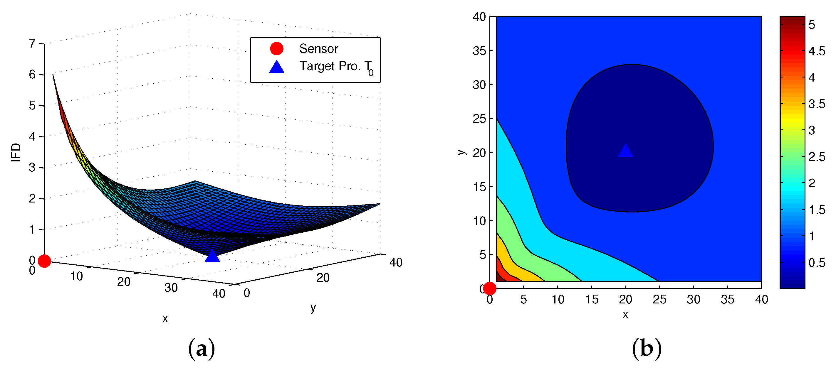
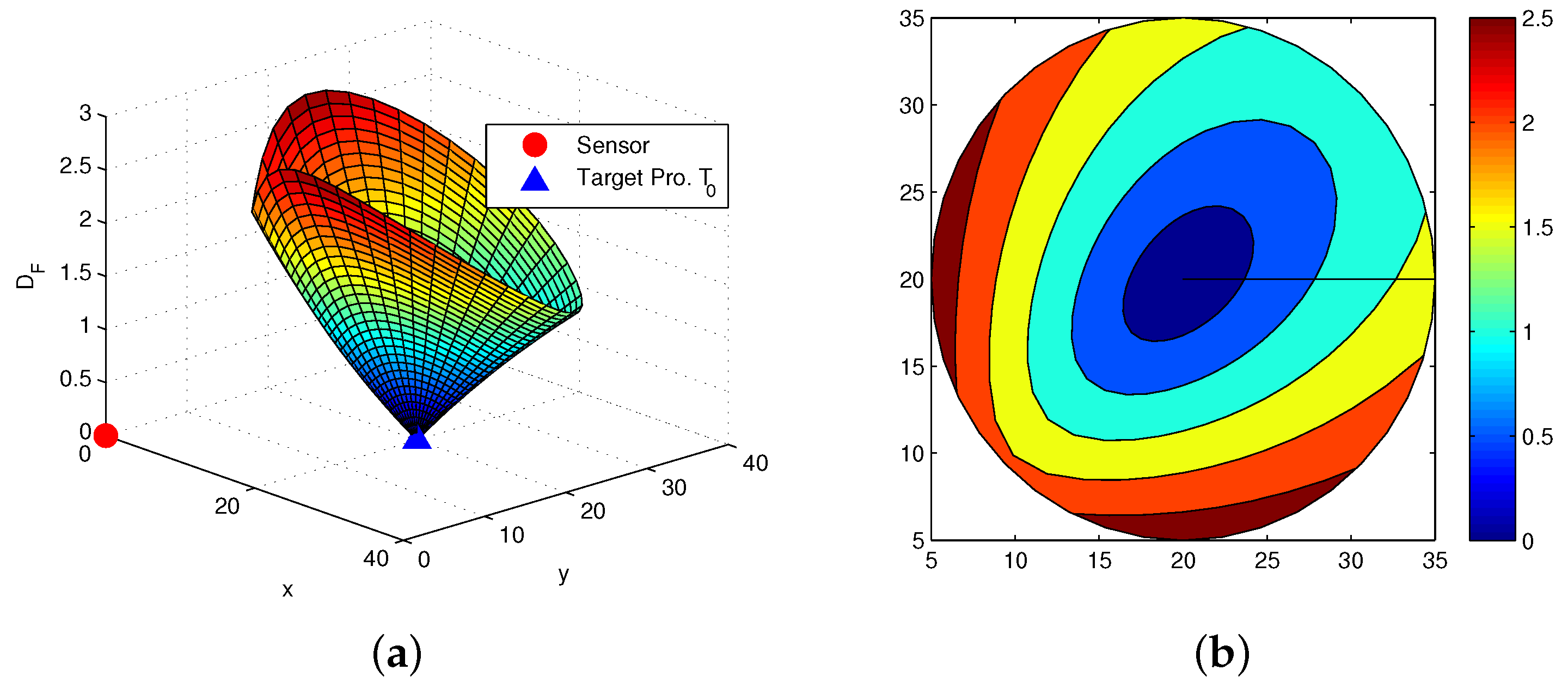
4.1. Information Resolution Based on Information Submanifold

In this subsection, the information resolution based on information submanifold is served as a new metric to measure the intrinsic similarities of the corresponding information matrix and is optimal to determine such resolution with respect to the underlying similitude which generates the manifold of SPD matrices based on differential geometry. It is defined on the basis of consideration of information distance connecting two relative FIMs for two measurement results. According to the definition, a new resolution cell denoted as $\mathsf{\Gamma }(\theta ,\delta )$ is a geodesic ball described by the set of equidistant points ${\theta }^{\prime }$ from the center θ in an information submanifold which is defined by a measurement model $\left\{p\right(x;\theta \left)\right\}$. Therefore, we have the following definition.

Definition 2.

For a given measurement model with pdf $p(x;\theta )$ and a known target state θ with $\delta >0$, the set

$$\begin{array}{c}\hfill \mathsf{\Gamma }(\theta ,\delta ):=\left\{{\theta }^{\prime }\right|d_p(G\left(\theta \right),G\left({\theta }^{\prime }\right))=\delta ,\delta \ge 0\},\end{array}$$

(51)

is called information resolution cell, where $d_p(G\left(\theta \right),G\left({\theta }^{\prime }\right))$ given by (32) is the IFD of the two targets and δ is the radius of the information resolution cell which is called the information resolution limit.

Given a minimal resolution limit value ${\delta }_0$ for a sensor network, we can distinguish two targets by the information resolution $d_p(G\left(\theta \right),G\left({\theta }^{\prime }\right))$, i.e., if $d_p(G\left(\theta \right),G\left({\theta }^{\prime }\right))>{\delta }_0$, the two targets can be distinguished, otherwise, we cannot distinguish them so that regard them as one target. In the following three subsections, we will use three classical measurement models, i.e., range-bearing measurement model, two-bearings measurement model and three dimensional (3D) range-bearings measurement model, to show the effectiveness of information resolution based on information submanifold.

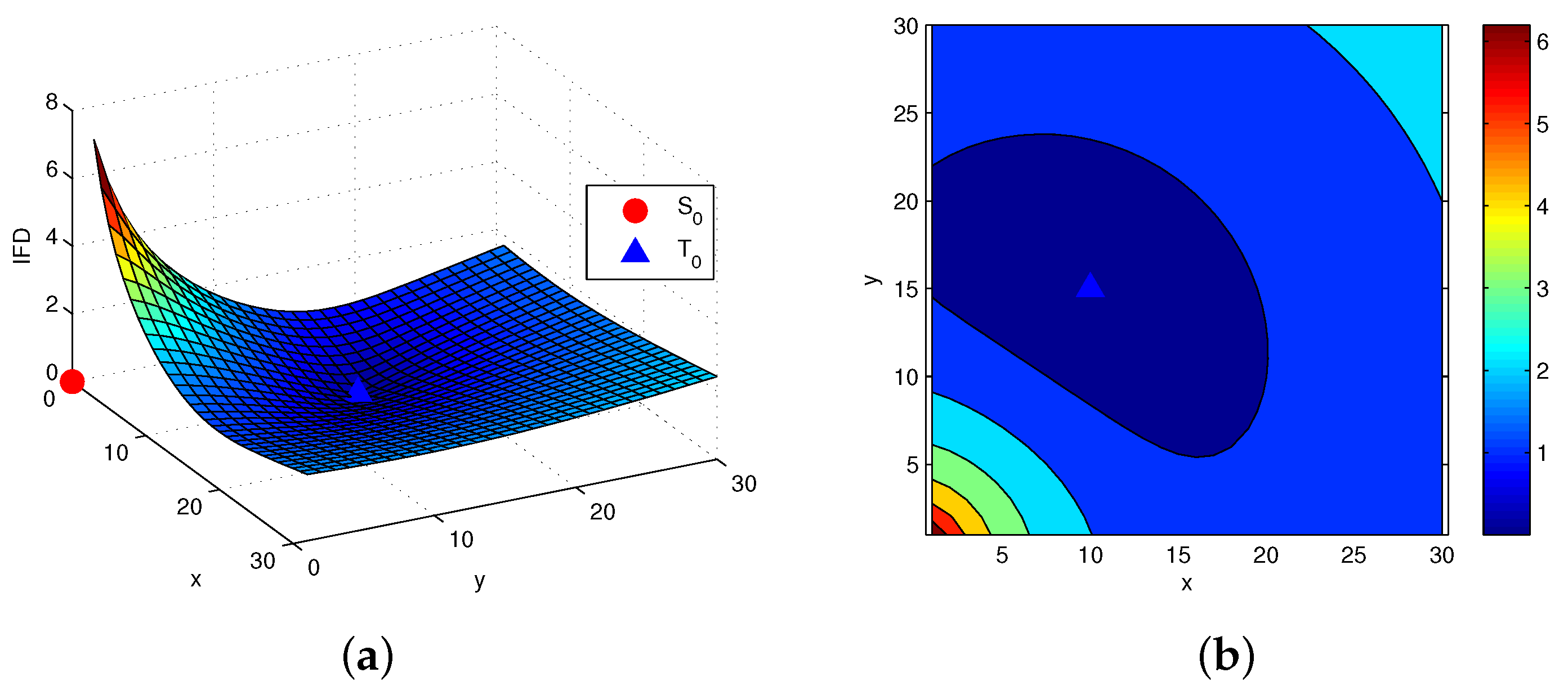
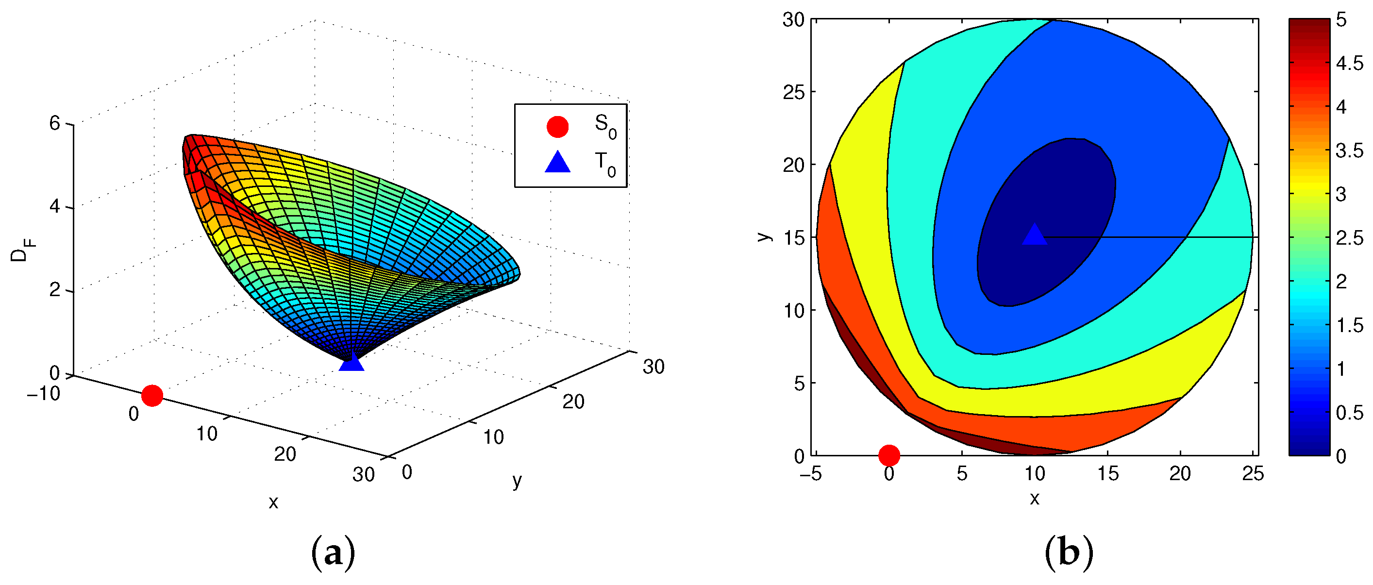
4.1.1. Range-Bearing Measurement

As well known that, assume that the sensor is located at the origin of coordinate $s_0=(0,0)$, the range-bearing measurement model can be represented as

$$\begin{array}{c}\hfill x=\left(\begin{array}{c}\tau \\ \phi \end{array}\right)=\left(\begin{array}{c}\sqrt{x^2+y^2}\\ arctan\frac{y}{x}\end{array}\right)+\left(\begin{array}{c}{w}_{\tau }\\ w_{\phi }\end{array}\right),\end{array}$$

(52)

where $w_{\tau }\sim N(0,r^4{\sigma }_{\tau }^2)$ with $r=\sqrt{x^2+y^2}$, $w_{\phi }\sim N(0,{\sigma }_{\phi }^2)$ and $\theta ={(x,y)}^T$. It should be noted that the term $r^4$ appeared in the diagonal of range component to take into account the fact that the amplitude of the radar echo signal attenuates according to the fourth power of the target range. Then, we can see that the sensor measurement x satisfies the Gaussian distribution with the mean and covariance matrix given by

$$\begin{array}{cc}\hfill \mu \left(\theta \right)=\left(\begin{array}{c}\sqrt{x^2+y^2}\\ arctan\frac{y}{x}\end{array}\right),C\left(\theta \right)& =\left(\begin{array}{cc}{r}^4{\sigma }_{\tau }^2& 0\\ 0& {\sigma }_{\phi }^2\end{array}\right).\hfill \end{array}$$

(53)

By (26), the corresponding FIM satisfies

$$\begin{array}{cc}\hfill g_{11}& =\frac{1}{{(x^2+y^2)}^2}\left[\frac{x^2}{(x^2+y^2){\sigma }_r^2}+\frac{y^2}{{\sigma }_{\phi }^2}+8x^2\right],\hfill \end{array}$$

(54)

$$\begin{array}{cc}\hfill g_{12}& =g_{21}=\frac{1}{{(x^2+y^2)}^2}\left[\frac{xy}{(x^2+y^2){\sigma }_r^2}-\frac{xy}{{\sigma }_{\phi }^2}+8xy\right],\hfill \end{array}$$

(55)

$$\begin{array}{cc}\hfill g_{22}& =\frac{1}{{(x^2+y^2)}^2}\left[\frac{y^2}{(x^2+y^2){\sigma }_r^2}+\frac{x^2}{{\sigma }_{\phi }^2}+8y^2\right].\hfill \end{array}$$

(56)

According to the FIM above, we can obtain an information submanifold corresponding to the range-bearing measurement model and calculate the information distance between any two measured target states for determining whether they can be resolved or not.

Assume that the area of interest is $30\times 30$ with ${\sigma }_{\tau }=1$ and ${\sigma }_{\phi }=0.2$. The sensor is located at $(0,0)$ and the known target $T_0$ is located at $(10,15)$. At the same time, without loss of generality, we assume that the detection target $T_t$ is on the same plane with $T_0$ and the sensor.

Figure 1a shows the information distance between two closely spaced targets $T_0$ and $T_t$ for range-bearing measurement sensor network. Figure 1b is the contour map of Figure 1a. A same plot is generated in Figure 2a in Rao geodesic distance based on information matrix metric ($D_F$). And the contour map generated via $D_F$ in the same scenario as in Figure 1b is given in Figure 2b. From this, we can see that the IFD increases with the area centered at the location of $T_0$. At the same time, we can know that the change of IFD is more larger when the detected target $T_t$ is closer to the sensor $S_0$. Clearly, the uncertainty area is under a given threshold to the value of IFD and target $T_t$ can be distinguished from target $T_0$ when it is outside this area. There are sixteen targets with Ed, $D_F$ and IFD as shown in

Table 1. $D_F$ and IFD with $T_0\left(T_0^{\prime }\right)$ for range-bearing measurement model.

$T_t$	(3,8)	(5,10)	(7,12)	(9,14)	(11,16)	(13,18)	(15,20)	(17,22)
Ed	9.90(7.07)	7.07(4.24)	4.24(1.41)	1.41(1.41)	1.41(4.24)	4.24(7.07)	7.07(9.90)	9.90(12.73)
$D_F$	1.28(1.12)	0.97(0.73)	0.62(0.26)	0.22(0.26)	0.22(0.73)	0.62(1.12)	0.97(1.47)	1.28(1.78)
IFD	2.15(1.67)	1.37(0.89)	0.74(0.27)	0.23(0.25)	0.21(0.69)	0.59(1.07)	0.93(1.40)	1.23(1.70)
$T_t$	(3,22)	(5,20)	(7,18)	(9,16)	(11,14)	(13,12)	(15,10)	(17,8)
Ed	9.90(10.30)	7.07(7.62)	4.24(5.10)	1.41(3.16)	1.41(3.16)	4.24(5.10)	7.07(7.62)	9.90(10.30)
$D_F$	2.73(3.65)	1.98(2.67)	1.19(1.61)	0.39(0.56)	0.39(0.72)	1.19(1.43)	1.98(2.21)	2.73(2.97)
IFD	0.94(1.26)	0.68(0.99)	0.41(0.73)	0.14(0.53)	0.14(0.48)	0.40(0.62)	0.65(0.85)	0.87(1.09)

corresponding to $T_0=(10,15)$ and $T_0^{\prime }=(8,13)$, respectively. It can be seen that the IFD is increasing with the Ed between $T_0$ and $T_t$, especially when $T_t$ is moving to close the sensor. Meanwhile, we can also know that the IFD is different for two detected targets with the same Ed to $T_0$, and the closer the Ed of one target to $S_0$ is, the bigger the IFD to $S_0$ is in generally. For example, setting $T_1=(3,8)$ and $T_8=(17,22)$ with the same $Ed=9.90$ and $D_F=1.28$ to $S_0$ for $T_0$, however the relationship of the IFD is $2.15>1.23$ which indicates that the presented information resolution is more efficient and accurate than others for this measurement system. In addition, if the minimal resolution limit ${\delta }_0$ is given as $0.25$ for the samples in Table 1, the four targets $T_4,T_5,T_{12}$ and $T_{13}$ cannot be distinguished with $T_0$, and the others can be distinguished. For target $T_0^{\prime }$, we can get the similar analysis results as $T_0$.

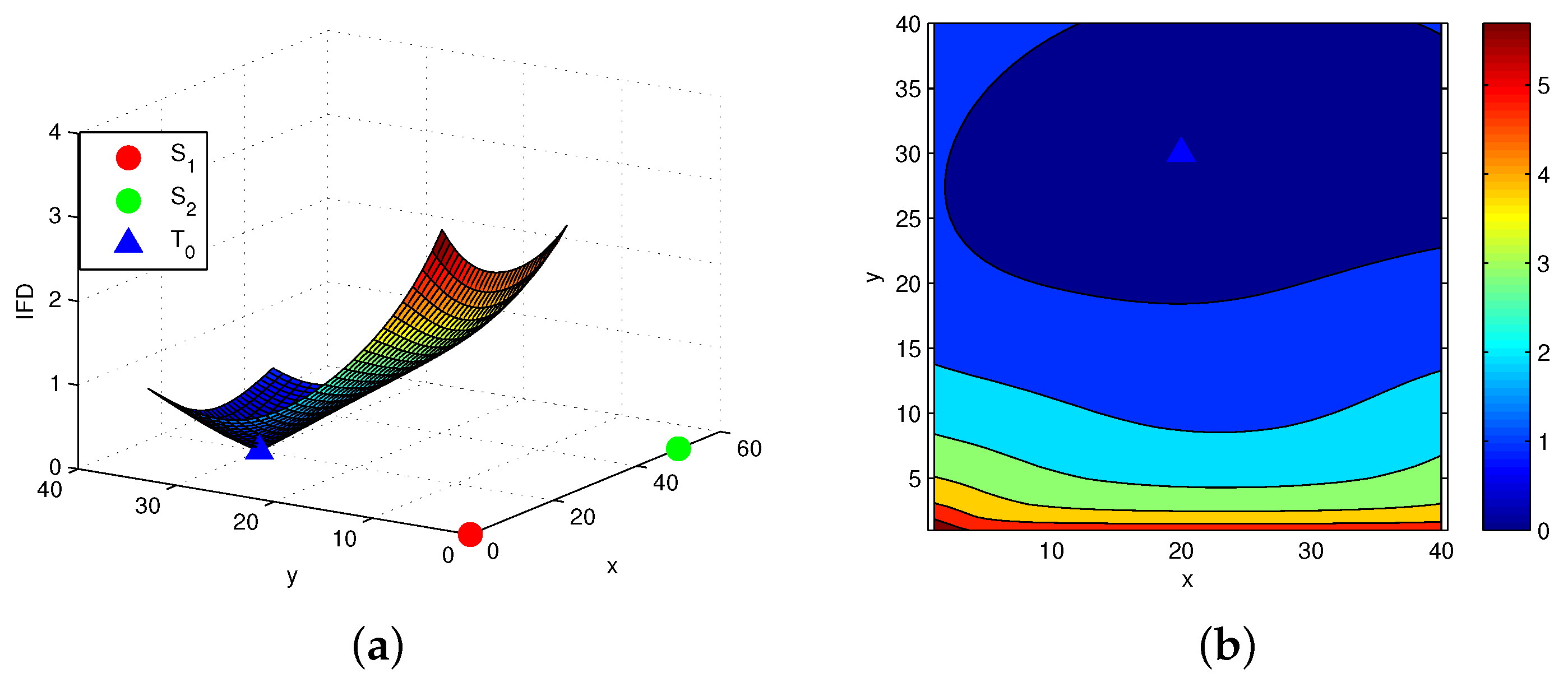
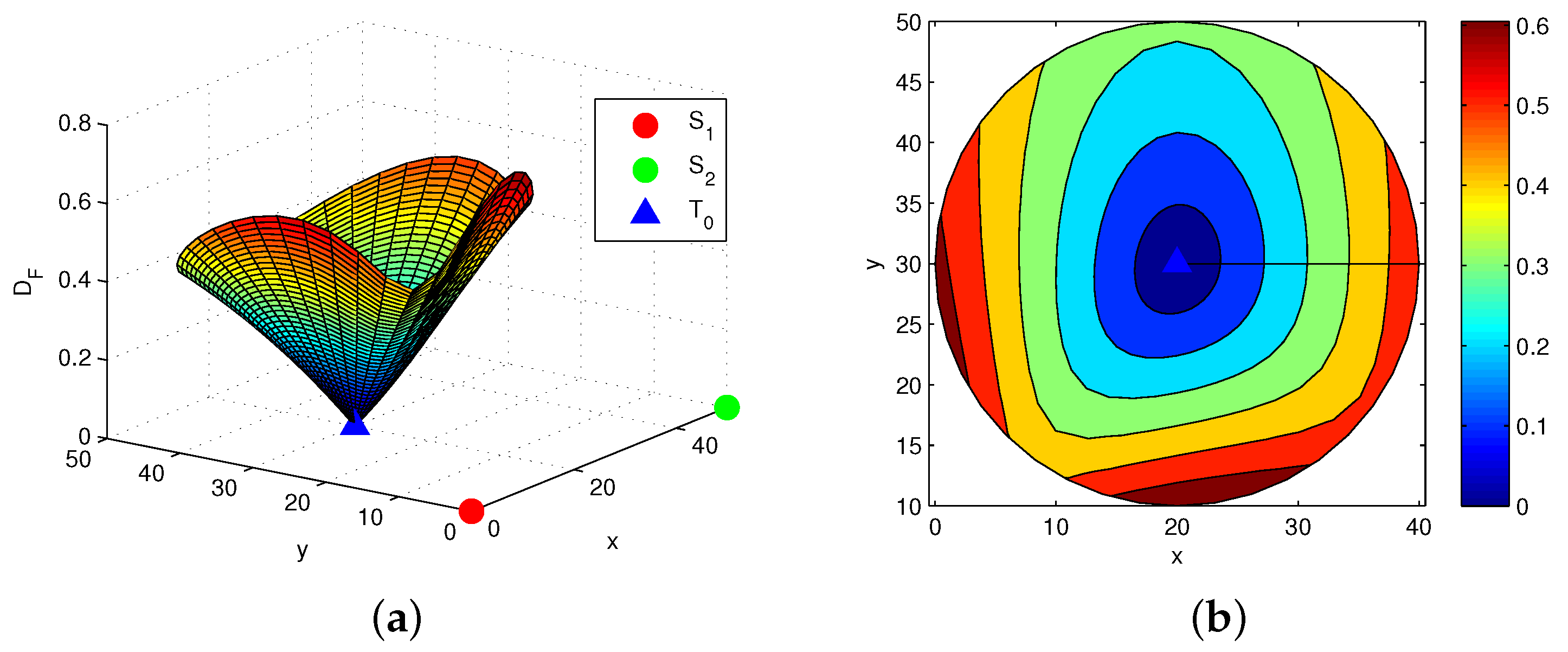
4.1.2. Two-Bearings Measurement

Suppose that two sensors $S_1$ and $S_2$ are located at $({\eta }_1,{\xi }_1)$ and $({\eta }_2,{\xi }_2)$ respectively. The sensors can observe two bearings of the target $T_0=(x,y)$ and each of the measurement ${\phi }_i$ satisfies the voM distribution, i.e.,

$$\begin{array}{c}\hfill {\phi }_i\sim voM({\mu }_i,\kappa ),\end{array}$$

(57)

where ${\mu }_i=arctan\frac{y-{\xi }_i}{x-{\eta }_i}$, and κ is a constant. Sine the sensor measurements are independent, each voM distribution is with common concentration parameter κ and the measurement at ith sensor has circular mean ${\phi }_i$, then the bearing measurements $\phi =({\phi }_1,{\phi }_2)$ satisfy the joint distribution with the pdf

$$\begin{array}{c}\hfill p(\phi ;\theta )=\frac{1}{2\pi I_0^2\left(\kappa \right)}exp\left\{\sum _{i=1}^2\kappa cos({\phi }_i-{\mu }_i)\right\},\end{array}$$

(58)

where $\theta ={(x,y)}^T$ is the local coordinate. Then, by (24), we can obtain the corresponding FIM as

$$\begin{array}{cc}\hfill g_{11}& =\kappa \frac{I_1\left(\kappa \right)}{I_0\left(\kappa \right)}\sum _{i=1}^2\frac{{(y-{\xi }_i)}^2}{{[{(x-{\eta }_i)}^2+{(y-{\xi }_i)}^2]}^2},\hfill \end{array}$$

(59)

$$\begin{array}{cc}\hfill g_{12}& =g_{21}=-\kappa \frac{I_1\left(\kappa \right)}{I_0\left(\kappa \right)}\sum _{i=1}^2\frac{(y-{\xi }_i)(x-{\eta }_i)}{{[{(x-{\eta }_i)}^2+{(y-{\xi }_i)}^2]}^2},\hfill \end{array}$$

(60)

$$\begin{array}{cc}\hfill g_{22}& =\kappa \frac{I_1\left(\kappa \right)}{I_0\left(\kappa \right)}\sum _{i=1}^2\frac{{(x-{\eta }_i)}^2}{{[{(x-{\eta }_i)}^2+{(y-{\xi }_i)}^2]}^2}.\hfill \end{array}$$

(61)

Thus, we can obtain an information submanifold corresponding to the two-bearings measurement model and calculate the information distance between two measured target states.

Assume that the area of interest is $50\times 50$ and $\kappa =9$. The two sensors are located at $S_1=(0,0)$, and $S_2=(50,0)$, respectively. The target $T_0$ is located at $(20,30)$. Without loss of generality, we also assume that the detection target $T_t$ is on the same plane with $T_0$ and the sensors.

Figure 3a shows the information distance between two spaced targets $T_0$ and $T_t$ for the two-bearings measurement sensor network. Figure 3b is the contour map of Figure 3a. A same plot is generated in Figure 4a in Rao geodesic distance based on information matrix metric. And the contour map generated via $D_F$ in the same scenario as in Figure 1b is given in Figure 4b. Accordingly, it is easy to know that the IFD increases with the area centered at the location of $T_0$. At the same time, we can know that the change of IFD is more larger when the detected target $T_t$ is closer to the line $\overline{S_1{S}_2}$ connecting the sensor $S_1$ and $S_2$. Clearly, the uncertainty area is under a given threshold to the value of IFD and target $T_t$ can be distinguished from target $T_0$ when it is outside this area. As shown in

Table 2. $D_F$ and IFD $T_0\left(T_0^{\prime }\right)$ for two-bearings measurement model.

$T_t$	(11,11)	(15,15)	(19,19)	(23,23)	(27,27)	(31,31)	(35,35)	(39,39)
Ed	21.0(15.2)	15.8(10.2)	11.1(6.3)	7.6(6.3)	7.6(10.2)	11.1(15.2)	15.8(20.3)	21.0(26.1)
$D_F$	0.38(0.53)	0.29(0.32)	0.21(0.16)	0.21(0.26)	0.21(0.33)	0.31(0.46)	0.43(0.60)	0.55(0.72)
IFD	1.88(1.71)	1.31(1.05)	0.90(0.59)	0.60(0.52)	0.38(0.81)	0.36(1.20)	0.58(1.59)	0.91(1.97)
$T_t$	(2,33)	(5,30)	(8,27)	(11,24)	(14,21)	(17,18)	(20,15)	(23,12)
Ed	18.3(28.0)	15.0(23.9)	12.4(19.7)	10.8(15.7)	10.8(11.7)	12.4(8.5)	15.0(5.4)	18.3(5.4)
$D_F$	0.53(0.64)	0.43(0.52)	0.34(0.46)	0.27(0.38)	0.23(0.30)	0.23(0.22)	0.47(0.17)	0.62(0.19)
IFD	1.05(2.07)	0.76(1.80)	0.56(1.55)	0.58(1.30)	0.76(1.04)	0.99(0.78)	1.24(0.54)	1.50(0.53)

with $T_0=(20,30)$ and $T_0^{\prime }=(25,17)$, for the selected samples, we can also get the similar property which is given in the last subsection. For example, setting $T_1=(11,11)$ and $T_8=(39,39)$ with the same $Ed=21.02$, the corresponding relationships about $D_F$ and IFD are $0.38<0.55$ and $1.88>0.91$, respectively. Thus, we can know that the presented information resolution has the same efficient as the Rao geodesic distance for the measurement model. Meanwhile, based on the geometrical property of this measurement model, i.e., the closer the detected target $T_t$ to the line $\overline{S_1{S}_2}$ is, the bigger the change of the Fisher information is, it can be seen that the presented method is more accuracy than others for this measurement model. Similarly, for a given minimal resolution limit ${\delta }_0=0.40$, there are only $T_5$ and $T_6$ which cannot be distinguished from $T_0$, while the all targets can be distinguished from $T_0^{\prime }$ under the same situations.

4.1.3. 3D Range-Bearings Measurement

Using a similar method, we consider the 3D positioning model in this subsection. Let the range, azimuth and altitude angle of the target $T(x,y,z)$ be τ, α and β, respectively. In the network of single conventional sensor measurement model, the state of a target is simply represented by its location, i.e., $\theta =(x,y,z)$. The sensor can observe range and bearings of the target, and then the measurement model can be written as

$$\begin{array}{c}\hfill x=\left(\begin{array}{c}\tau \\ \alpha \\ \beta \end{array}\right)=\left(\begin{array}{c}\sqrt{x^2+y^2+z^2}\\ arctan\frac{y}{x}\\ arctan\frac{z}{\sqrt{x^2+y^2}}\end{array}\right)+\left(\begin{array}{c}{w}_{\tau }\\ w_{\alpha }\\ w_{\beta }\end{array}\right),\end{array}$$

(62)

where τ, α and β denote the range, angle of rotation and angle of altitude of the measurement subject to an additive zero-mean Gaussian noise $\omega =[{\omega }_{\tau },{\omega }_{\alpha },{\omega }_{\beta }]$ with the covariance $C\left(\theta \right)$, respectively. Therefore, the measurement x obeys a normal distribution with the mean and the covariance respectively satisfying

$$\begin{array}{c}\hfill \mu \left(\theta \right)=\left(\begin{array}{c}\sqrt{x^2+y^2+z^2}\\ arctan\frac{y}{x}\\ arctan\frac{z}{\sqrt{x^2+y^2}}\end{array}\right),C\left(\theta \right)=\left(\begin{array}{ccc}{R}^4{\sigma }_{\tau }^2& 0& 0\\ 0& {\sigma }_{\alpha }^2& 0\\ 0& 0& {\sigma }_{\beta }^2\end{array}\right),\end{array}$$

(63)

where $R=\sqrt{x^2+y^2+z^2}$, ${\sigma }_{\tau },{\sigma }_{\alpha }$ and ${\sigma }_{\beta }$ are the standard deviations of range and bearings measurement noise, respectively. By (26), we can calculate the FIM elements of model (62) respectively as follows

$$\begin{array}{cc}\hfill g_{11}=& \frac{x^2}{R^4}\left[\frac{1}{R^2{\sigma }_{\tau }^2}+\frac{z^2}{(x^2+y^2){\sigma }_{\beta }^2}+8\right]+\frac{y^2}{{(x^2+y^2)}^2{\sigma }_{\alpha }^2},\hfill \end{array}$$

(64)

$$\begin{array}{cc}\hfill g_{22}=& \frac{y^2}{R^4}\left[\frac{1}{R^2{\sigma }_{\tau }^2}+\frac{z^2}{(x^2+y^2){\sigma }_{\beta }^2}+8\right]+\frac{x^2}{{(x^2+y^2)}^2{\sigma }_{\alpha }^2},\hfill \end{array}$$

(65)

$$\begin{array}{cc}\hfill g_{33}=& \frac{z^2}{R^4}\left(\frac{1}{R^2{\sigma }_{\tau }^2}-\frac{1}{{\sigma }_{\beta }^2}+8\right)+\frac{1}{{\sigma }_{\beta }^2},\hfill \end{array}$$

(66)

$$\begin{array}{cc}\hfill g_{12}=& g_{21}=\frac{xy}{R^4}\left[\frac{1}{R^2{\sigma }_{\tau }^2}+\frac{z^2}{(x^2+y^2){\sigma }_{\beta }^2}+8\right]-\frac{xy}{{(x^2+y^2)}^2{\sigma }_{\alpha }^2},\hfill \end{array}$$

(67)

$$\begin{array}{cc}\hfill g_{13}=& g_{31}=\frac{xz}{R^4}\left(\frac{1}{R^2{\sigma }_{\tau }^2}-\frac{1}{{\sigma }_{\beta }^2}+8\right),\hfill \end{array}$$

(68)

$$\begin{array}{cc}\hfill g_{23}=& g_{32}=\frac{yz}{R^4}\left(\frac{1}{R^2{\sigma }_{\tau }^2}-\frac{1}{{\sigma }_{\beta }^2}+8\right),\hfill \end{array}$$

(69)

By the six equations above, we can calculate the geodesic distance between any two information matrices corresponding to the 3D measurement model. Assume that the area of interest is $40\times 40\times 50$, ${\sigma }_{\tau }=1$, and ${\sigma }_{\alpha }={\sigma }_{\beta }=0.2$. Then, the sensor is located at $(0,0,0)$, and the reference target is located at $(20,20,20)$. In addition, we assume that the moving target is on the same plane with $z=20$ for simplifying the simulation results.

Figure 5a shows the information distance between two closely spaced targets $T_0$ and $T_t$ for 3D range and angle measurement sensor network and Figure 5b is the contour map of Figure 5a. From this we can know that the IFD increases with the area centered at the location of $T_0$. The closer that target $T_t$ to $T_0$ is, the smaller the IFD is. For a given resolution limit ${\delta }_0$, we can easily know that two targets whether can be distinguished or not by calculating the IFD between them, i.e., there are two detection points or one point. A same plot is generated in Figure 6a in Rao geodesic distance based on information matrix metric. And the contour map generated via $D_F$ in the same scenario is given in Figure 6b. For some samples as shown in

Table 3. $D_F$ and IFD with $T_0\left(T_0^{\prime }\right)$ for 3D range-bearings measurement sensor network.

$T_t$	(6,6,6)	(10,10,10)	(14,14,14)	(18,18,18)	(22,22,22)	(26,26,26)	(30,30,30)	(34,34,34)
Ed	24.3(17.3)	17.3(10.4)	10.4(3.5)	3.5(3.5)	3.5(10.4)	10.4(17.3)	17.3(24.3)	24.3(31.2)
$D_F$	70.0(50.0)	50.0(30.0)	30.0(10.0)	10.0(10.0)	10.0(30.0)	30.0(50.0)	50.0(70.0)	70.0(90.0)
IFD	2.41(1.96)	1.3(0.94)	0.71(0.27)	0.21(0.24)	0.19(0.64)	0.52(0.97)	0.81(1.26)	1.06(1.51)
$T_t$	(6,6,34)	(10,10,30)	(14,14,26)	(18,18,22)	(22,22,18)	(26,26,14)	(30,30,10)	(34,34,6)
Ed	24.3(22.9)	17.3(16.4)	10.4(10.4)	3.5(6.6)	3.5(8.7)	10.4(14.3)	17.3(20.7)	24.3(27.4)
$D_F$	70.0(90.0)	50.0(70.0)	30.0(50.0)	10.0(30.0)	10.0(10.0)	30.0(10.0)	50.0(30.0)	70.0(50.0)
IFD	2.47(1.96)	1.49(0.95)	0.84(0.27)	0.27(0.36)	0.26(0.89)	0.76(1.39)	1.20(1.83)	1.58(2.21)

with $T_0=(20,20,20)$ and $T_0^{\prime }=(16,16,16)$, the similar analysis results can be also obtained as the 2D range-bearing measurement model. For example, by a given minimal resolution limit ${\delta }_0=0.25$, there are only $T_4$ and $T_5$ which cannot be distinguished from $T_0$ and only $T_4$ which cannot be distinguished from $T_0^{\prime }$ with the presented method.

Remark 1.

From the analysis with the three sensor systems above, it illustrates the sensing ability of the sensor networks to distinguish two closely spaced targets. A minimal detectable information distance may be identify in the maps for a given resolution limit ${\delta }_0$. If information distance between two targets is below the given threshold, the two closely spaced targets may not be distinguished by the sensor system and are considered as one target. Otherwise, we can distinguish them as two different targets. In addition, compared with some classical resolution, information resolution based on information submanifold and information resolution based on statistical manifold are all defined throughout geodesic distance and can all show the geometric property of sensor networks measurement system. It should be noted that, because there is no explicit geodesic expression on statistical manifold in general, the geodesic calculation has very high complexity and is approximately handled by the Euclidean distance sometimes. Thus, it would be some cause of calculation error for target resolvability, especially when the two targets is not fairly close to each other. However, the information distance based on information submanifold is only related to FIMs corresponding to the targets states and can be calculated by an explicit geodesic expression on $PD\left(n\right)$. Meanwhile, the presented resolution in this paper can show the Fisher information and the measurement models more effectively.

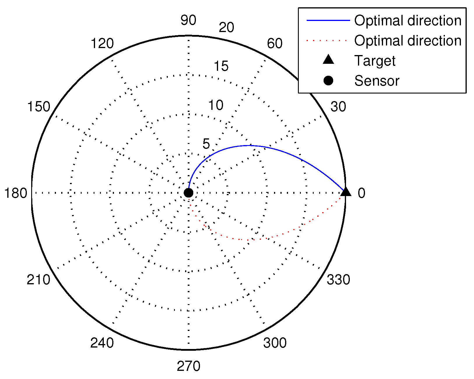
4.2. Bearing-Only Tracking With Single Sensor

In this subsection, we present a new tracking method based on information submanifold for bearing-only tracking with a single sensor. By (59)∼(62), as a function of the second sensor location, the determinant of the FIM can be given by

$$\begin{array}{c}\hfill f({\eta }_2,{\xi }_2)={\left[\frac{\kappa I_1\left(\kappa \right)({\tilde{x}}_1{\tilde{y}}_2-{\tilde{x}}_2{\tilde{y}}_1)}{I_0\left(\kappa \right)R_1^2{R}_2^2}\right]}^2,\end{array}$$

(70)

where ${\tilde{x}}_1=x-{\eta }_1,{\tilde{x}}_2=x-{\eta }_2,{\tilde{y}}_1=y-{\xi }_1,{\tilde{y}}_2=y-{\xi }_2$, and $R_i={(x-{\eta }_i)}^2+{(y-{\xi }_i)}^2$.

For the given locations of the two sensors, we can get the Fisher information for the detection target by (70) which represents the volume of the amount of information. Under the same situation as in the last subsection, the target information map and the contour map for the two-bearings passive sensor networks can be obtained as shown in Figure 7a,b on a logarithm scale. From the two figures, it can be seen that the amount of the information is very little and even almost is zero nearby the straight line passing through the two sensors. In fact, the target can not be located in this region due to the bearing-only measurement. In order to eliminate the unmeasurable area and obtain the maximal Fisher information, we can move the sensor with respect to the target. If the trajectory of the target moving is known, the sensor would have an optimal scheduling such that maximal target information. Therefore, we make the following parameter replacement using the polar coordinate

$$\begin{array}{c}\hfill \left\{\begin{array}{cc}{\eta }_2={\eta }_1+rcos\phi ,\hfill & \hfill \\ {\xi }_2={\xi }_1+rsin\phi ,\hfill & \hfill \end{array}\right.\end{array}$$

(71)

where r and $\phi$ denote the step length and the direction of the sensor movement, respectively. Substituting (71) into (70), we see that (70) becomes

$$\begin{array}{c}\hfill f(r,\phi )={\left\{\frac{\kappa I_1\left(\kappa \right)[{\tilde{x}}_1({\tilde{y}}_1-rsin\phi )-({\tilde{x}}_1-rcos\phi ){\tilde{y}}_1]}{I_0\left(\kappa \right)R_1^2[R_1^2-2r({\tilde{x}}_{1}cos\phi +{\tilde{y}}_{1}sin\phi )+r^2]}\right\}}^2.\end{array}$$

(72)

Taking the partial derivative of (72) with respect to $\phi$ and setting it to be zero, we can obtain the optimal sensor heading course ${\phi }_{opt}$ which satisfies the following expression

$$\begin{array}{c}\hfill tan{\phi }_{opt}=\frac{\frac{|r^2-R_1|}{2r{R}_1}+\frac{{\tilde{y}}_1}{{\tilde{x}}_1}}{1-\frac{|r^2-R_1|}{2r{R}_1}·\frac{{\tilde{y}}_1}{{\tilde{x}}_1}}.\end{array}$$

(73)

Without loss of generality, let the Line-of-Sight from the sensor to the target be the baseline direction of the coordinate systems. The optimal sensor moving direction based on (73) can be simplified as

$$\begin{array}{c}\hfill {\phi }_{opt}=\pm arctan\frac{|r^2-R_1^2|}{2r{R}_1}=\pm arctan\frac{|{\lambda }^2-1|}{2\lambda },\end{array}$$

(74)

where $\lambda =r/R_1$.

Assume that the initial state of the sensor locates at $(0,0)$, and the location of the target is $(10,0)$. Then, we can get the polar relation map about the optimal moving direction ${\phi }_{opt}$ and the moving radius r as Figure 8.

As described in Figure 8, the optimal direction of the sensor changes from ${90}^{\circ }$ to $0^{\circ }$ with the increase of the length of tracking radius. And when the radius equals to the distance between the target and the sensor, i.e., $r=R_1$, the optimal direction is $0^{\circ }$. Therefore, we can select the optimal direction based on the radius of the sensor which we design in the practical applications.

5. Conclusions

In this paper, we have proposed the information submanifold and its applications for sensor networks based on SPD matrices. Three simple examples corresponding three probability distributions are calculated with the geodesic and geodesic distance. The problems of target resolution and tracking with a single sensor based on the information submanifold are analyzed and computed through two classical sensor networks models. The simulation results have shown that the proposed method yields very effective performance in practical environments. Our future work will focus on the applications of the curvature of the information submanifold for the management and tracking of the sensor networks.

References

1. Fiori, S. Learning the Fre’chet Mean over the Manifold of Symmetric Positive-Definite Matrices. Cognit. Comput. 2009, 1, 279–291. [Google Scholar] [CrossRef]
2. Harandi, M.T.; Salzmann, M.; Hartley, R. From Manifold to Manifold: Geometry-Aware Dimensionality Reduction for SPD Matrices; Springer: Basel, Switzerland, 2014; Volume 8690, pp. 17–32. [Google Scholar]
3. Arsigny, V.; Fillard, P.; Pennec, X.; Ayache, N. Geometric Means in a Novel Vector Space Structures on Symmetrics Positive-Definite Matrices. Siam J. Matrix Anal. Appl. 2007, 29, 328–347. [Google Scholar] [CrossRef]
4. Le Bihan, D. Diffusion MNR Imaging. Magn. Reson. Q. 1991, 7, 1–30. [Google Scholar] [PubMed]
5. Fillard, P.; Arsigny, V.; Pennec, X.; Hayashi, K.M.; Thompson, P.M.; Ayache, N. Measuring Brain Variability by Extrapolating Sparse Tensor Fields Measured on Sulcal Lines. Neuroimage 2007, 34, 639–650. [Google Scholar] [CrossRef] [PubMed]
6. Harandi, M.T.; Sanderson, C.; Hartley, R.; Lovell, B.C. Sparse Coding and Dictionary Learning for Symmetric Positive Definite Matrices: A Kernel Approach. Lect. Notes Comput. Sci. 2012, 7573, 216–229. [Google Scholar]
7. Jayasumana, S.; Hartley, R.; Salzmann, M.; Li, H.; Harandi, M. Kernel Methods on the Riemannian Manifold of Symmetric Positive Definite Matrices. In Proceedings of the 2013 IEEE Conference on Computer Vision and Pattern Recognition, Portland, OR, USA, 23–28 June 2013; pp. 73–80.
8. Moakher, M. A Differential Geometric Approach to The Geometric Mean of Symmetric Positive-Definite Matrices. Siam J. Matrix Anal. Appl. 2005, 26, 735–747. [Google Scholar] [CrossRef]
9. Hall, B. Lie Groups, Lie Algebras, and Representations: An Elementary Introduction; Springer: Berlin/Heidelberg, Germany, 2003. [Google Scholar]
10. Menendez, M.L.; Morales, D.; Pardo, L.; Salicrij, M. Statistical Test Based on Geodesic Distances. Appl. Math. Lett. 1995, 8, 65–69. [Google Scholar] [CrossRef]
11. Fiori, S. A Theory for Learning by Weight Flow on Stiefel-Grassman Manifold. Neural Comput. 2001, 13, 1625–1647. [Google Scholar] [CrossRef]
12. Fiori, S. Solving Minimal-Distance Problems over the Manifold of Real-Symplectic Matrices. Siam J. Matrix Anal. Appl. 2011, 32, 938–968. [Google Scholar] [CrossRef]
13. Bini, D.A.; Iannazzo, B. Computing the Karcher Mean of Symmetric Positive Definite Matrices. Stat. Methodol. 2007, 4, 341–353. [Google Scholar] [CrossRef]
14. Barbaresco, F. Interactions Between Symmetric Cones and Information Geometrics: Bruhat-Tits and Siegel Spaces Models for High Resolution Autregressive Doppler Imagery. Springer Lect. Notes Comput. Sci. 2009, 5416, 124–163. [Google Scholar]
15. Barbaresco, F. Innovative Tools for Radar Signal Processing based on Cartan’s Geometry of SPD Matrices and Information Geometry. In Proceedings of the IEEE Radar Conference, Rome, Italy, 26–30 May 2008; pp. 26–30.
16. Nielsen, F.; Bhatia, R. Matrix Information Geometry; Springer: Berlin/Heidelberg, Germany, 2013. [Google Scholar]
17. Mahata, K.; Schoukens, J.; de Cock, A. Information Matrix and D-optimal Design with Gaussian Inputs for Wiener Model Identification. Automatica 2016, 69, 65–77. [Google Scholar] [CrossRef]
18. Stoica, P.; Marzetta, T.L. Parameter Estimation Problems with Singular Information Matrices. IEEE Trans. Signal Proc. 2001, 49, 87–90. [Google Scholar] [CrossRef]
19. Amari, A.; Weiss, A.J. Fundamental resolution limits of closely spaced random signals. IET Radar Sonar Navig. 2008, 2, 170–179. [Google Scholar] [CrossRef]
20. Amari, A.; Weiss, A.J. Fundamental limitations on the resolution of deterministic signals. IEEE Trans. Signal Proc. 2008, 56, 5309–5318. [Google Scholar] [CrossRef]
21. Hero, A.O., III; Castañón, D.; Cochran, D.; Kastella, K. Foundations and Applications of Sensor Management; Springer: New York, NY, USA, 2008. [Google Scholar]
22. Nardone, S.C.; Aidala, V.J. Observability Criteria for Bearings-Only Target Motion Analysis. IEEE Trans. Autom. Control 1981, 17, 162–166. [Google Scholar] [CrossRef]
23. Jauffret, C.; Pillon, D. Observability in Passive Target Motion Analysis. IEEE Trans. Aerosp. Electron. Syst. 1996, 32, 1290–1300. [Google Scholar] [CrossRef]
24. Cheng, Y.; Wang, X.; Caelli, T.; Li, X.; Moran, B. On Information Resolution of Radar Systems. IEEE Trans. Aerosp. Electron. Syst. 2012, 48, 3084–3102. [Google Scholar] [CrossRef]
25. Cheng, Y.; Wang, X.; Moran, B. Sensor Network Performance Evaluation in Statistical Manifolds. In Proceedings of the 2010 13th Conference on Information Fusion (FUSION), Edinburgh, UK, 26–29 July 2010.
26. Barton, D.K.; Leonov, S.A. Radar Technology Encyclopedia; Artech House: Massachusetts, MA, USA, 1997. [Google Scholar]
27. Amari, S.; Nagaoka, H. Methods of Information Geometry; American Mathematical Society: Providence, RI, USA, 2000. [Google Scholar]
28. Lang, S. Foundations of Differential Geometry; Springer: New York, NY, USA, 1999. [Google Scholar]
29. Amari, S. Differential Geometry of Curved Exponential Families-Curvatures and Information Loss. Ann. Stat. 1982, 10, 357–385. [Google Scholar] [CrossRef]
Figure 1. (a) IFD between two closely spaced targets for range-bearing measurement model; (b) The contour map of Figure 1a.
Entropy 19 00131 g001
Figure 2. (a) D F between two closely spaced targets for range-bearing measurement model; (b) The contour map of Figure 2a.
Entropy 19 00131 g002
Figure 3. (a) IFD between two closely spaced targets for two-bearings measurement model; (b) The contour map of Figure 3a.
Entropy 19 00131 g003
Figure 4. (a) D F between two closely spaced targets for two-bearings measurement model; (b) The contour map of Figure 4a.
Entropy 19 00131 g004
Figure 5. (a) D F between two closely spaced targets for 3D range-bearings measurement sensor network; (b) The contour map of Figure 5a.
Entropy 19 00131 g005
Figure 6. (a) D F between two closely spaced targets for 3D range-bearings measurement sensor network; (b) The contour map of Figure 6a.
Entropy 19 00131 g006
Figure 7. (a) Target information for the sensor network with two-bearings passive sensor networks; (b) The contour map of target information.
Entropy 19 00131 g007
Figure 8. Optimal sensor movement direction for given radius.
Entropy 19 00131 g008