Quaternion Entropy for Analysis of Gait Data


Institute of Informatics, Silesian University of Technology, Akademicka 16, 44-100 Gliwice, Poland
Entropy 2019, 21(1), 79; https://doi.org/10.3390/e21010079
Submission received: 9 December 2018
/
Revised: 9 January 2019
/
Accepted: 15 January 2019
/
Published: 17 January 2019
(This article belongs to the Special Issue Information Theory Applications in Signal Processing)
Abstract
:Nonlinear dynamical analysis is a powerful approach to understanding biological systems. One of the most used metrics of system complexities is the Kolmogorov entropy. Long input signals without noise are required for the calculation, which are very hard to obtain in real situations. Techniques allowing the estimation of entropy directly from time signals are statistics like approximate and sample entropy. Based on that, the new measurement for quaternion signal is introduced. This work presents an example of application of a nonlinear time series analysis by using the new quaternion, approximate entropy to analyse human gait kinematic data. The quaternion entropy was applied to analyse the quaternion signal which represents the segments orientations in time during the human gait. The research was aimed at the assessment of the influence of both walking speed and ground slope on the gait control during treadmill walking. Gait data was obtained by the optical motion capture system.
1. Introduction
The parameters associated with chaos are measures of dimension, rate of information (entropy) and the Lyapunov determinant. Kolmogorov entropy K is known as a chaos metrics and the value of entropy can be used for the classification of underling dynamic systems [1]. The connection of Kolmogorov entropy and Lyapunov determinants of the system is defined by Pessin’s theorem. Sensitive dependence on initial conditions is a distinguishing feature of chaotic behavior. Initially, arbitrarily close points in the phase space produce significantly different trajectories. Characteristically, trajectories in chaotic systems diverge exponentially and Lyapunov exponents () were proved to be a good quantitative measure for the average rate of exponential divergence of two trajectories. Hence, positive is indicative of unpredictable behavior. K is basically equal to the sum of the positive of the system.
Theoretical defined entropy K is not able to be obtained on a base on finite, noisy data (signals) obtained from real measurements. The amount of data typically required to archive convergence is between to points to fill out a d-dimensional strange attractor for the chaotic system [2]. To overcome this, the approximate entropy, as a family of statistics, has been proposed [3]. It was shown that it can potentially distinguish low dimensional deterministic systems, periods and multiply periodic, high dimensional chaotic, stochastic and mixed systems [4]. The approximate entropy statistics is based on an Eckmann–Ruelle entropy formula [5], for the physical invariant measure for use with time series data.
This work presents the new quaternion, approximate entropy and its application to analysis of human gait kinematic data represented as a quaternion signal. This signal represents the segments orientations in time during the human gait. The research was aimed at the assessment of the influence of both walking speed and ground slope on the proposed quaternion entropy during treadmill walking. Gait data was obtained by the optical motion capture system. The analysis was carried out for femur, tibia and foot segments.
2. Materials and Methods
2.1. Background
Letting be a time series signal of measurements equally spaced in time, the sequence of vectors in can be defined as , where . Next, for each i and j, , and , the following function is defined as
where # is the number of elements in set, r is vector comparison distance and m is the dimension of created and compared vectors. The distance d is defined as follows:
The definitions above are based on correlation dimension derivation and are needed to define as
Given N samples, we can define the following formula as statistics:
Informally, given N signal’s samples, the family of statistics is a measure of probability that two sequences that are similar for m points remain similar, that is, within a tolerance r, in the next sample in a signal. Thus, a low value of reflects a high degree of regularity. Following family statistics, has been widely used in clinical cardiovascular studies [6,7,8,9] and neurology, among others, for analysis of electroencephalogram signals [10,11,12,13].
Similar derivation has related to complexity measure sample entropy () [6]. Sample entropy in counting the similar vectors does not count self-matches. The entropy algorithm counts each sequence as matching itself, which is a way to avoid occurrence of in calculations. In practice, this causes some bias value in results. This was a very detailed discussion in [6,14]. However, and also indicate more self-similarity in the time series.
Entropy to gait analysis was used only for times series consisting of spatio-temporal parameters like step time, length and width, stride intervals [14,15] or segment trajectories [16]. Analysis of center of COP (center of pressure) trajectory by sample entropy can be found in [17]. In [18], multiscale entropy [19] was applied on trunk acceleration data collected during a gait of subjects of different ages: toddlers, pre-scholar and scholar children, adolescents, young adults, adults and elderlies. Control entropy was used to analyse the acceleration data as three independent signals [20]. Each cited entropy used to analyse gait data is based on formula.
Based on actual knowledge, there is no proposition to compute entropy to analyse gait data based on unit quaternions’ time series. This conception allows for processing correlated data and to obtain results taking into account rotations in 3D. The same preliminary studies were done based on quaternion energy and entropy to the classification of people based on gait data [21].
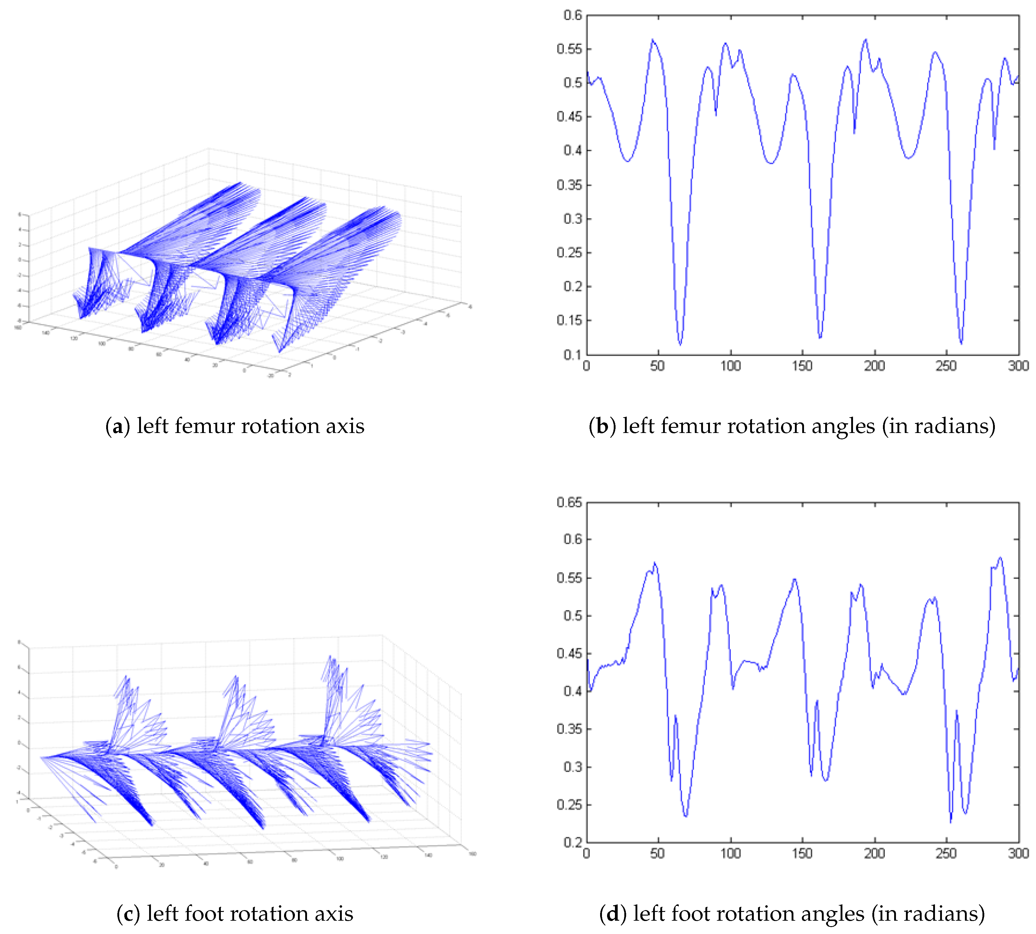
In [22], the authors describe an example of application of a nonlinear time series analysis directed at identifying the presence of deterministic chaos in human gait kinematic data by means of the largest Lyapunov exponent (). A positive value is interpreted as an indicator of local instability. However, the was computed based on separate Euler angles (three rotations angles about the axes of a coordinate system) or only angles of rotation in quaternion representation. Such analysis in quaternion form did not consider axis of rotation. In this research experiment, data from this same trial was used so the results will be compared. Figure 1a,c present the axis of rotation (imaginary part of quaternion) during 300 samples of gait (about 3 strides). Figure 1b,d show the angle of rotation (scalar part of quaternion). To analyse all aspects of movement during gait, all of the information should be processed. The new propositions of quaternion motion analysis tools are widely discussed in [23,24,25,26].
The o orientation indicates the orientation of the rigid body defined in the reference system (also named as the reference frame). Rotation means a change in orientation, . The group (special orthogonal group) contains all rotations around the origin of the Euclidean coordinate system . Rotations can be described by orthogonal matrices. Rotations can also be written as a combination of three Euler angles around the three coordinate system axes. The angles are usually referred to as roll, pitch and yaw. In this representation, the order in which the rotation is performed is important. There is also the phenomenon of blocking one degree of freedom of movement (gimbal lock).
In computer graphics, the most common description of rotation is unit quaternion [27,28]. Quaternions [27,28] are an extension of complex numbers, where is a quaternion algebra. Quaternion , consists of real and imaginary part . Multiplication of two quaternions is marked as ⊗. We can write quaternion as vector and scalar part: . Using the Euler rule for complex numbers, we have a rotation around the axis by an angle :
In order to represent the rotation, unit quaternions are used, which fulfill the condition , where is a scalar product. Unit quaternions lie on the hypersphere (denoted as ) embedded in Euclidean space 4D. The space is a map with double mapping. This means that each rotation (or orientation) can be represented by two unit quaternions, called antipode. They represent a rotation around this same axis, but with a positive or negative angle. Conjunction quaternion represents inverse rotation , which for unit quaternions is equal to inverse quaternion .
In summary, unit quaternions are a suitable mathematical tool for describing orientation and rotation in 3D space. It is possible to describe the rotation composition as multiplying quaternions. Conjunction quaternion represents inverse rotation. Such a description is free from the phenomenon of blocking one degree of freedom. The distance metrics between quaternions [29,30] have also been defined.
Using quaternions and building analysis in the domain , we can process rotational data as correlated data with simultaneous rotation information around each axis of rotation. It also eliminates the problem of blocking one degree of freedom (gimbal lock) and allows a consistent mathematical record.
2.2. Quaternion Approximate Entropy
Let us assume that input a motion signal consists of quaternions: where and for some .
Furthermore, the signal is processed by the selective negation (hemispherization), that is, every quaternion is converted to if due to duality of unit quaternions which represent rotations. It satisfies the requirement according to which two adjacent quaternions are located on the same hemisphere.
The new proposed metric, the quaternion, approximate entropy , is based on Equation (5). Quaternions are of unit length, which means they are located only on a hypersphere . Thus, to compare rotations, it is sufficient to calculate cosine distances between related quaternions, which is reflected by angles between vectors formed by quaternions’ components. The scalar product can be used to accomplish the task:
The distance between two quaternions in Equation (2) is defined as , so the equation is:
2.3. Treadmill Experiments
Time series were extracted from treadmill gait sequences which were recorded in the Human Motion Laboratory (HML) of the Polish-Japanese Academy of Information Technology (Bytom, Poland) by the optical motion capture system. Data was recorded with the use of the Vicon Nexsus optical motion capture system (Vicon Motion Systems Ltd., Oxford, UK). The skeleton model of 22 segments is applied and positions are traced based on 39 markers in standard full body Plug-In Gait marker placement. For analysis, only Euler angles’ orientations of femur, tibia, foot (left and right) segments were converted to unit quaternions time series signal.
Application of the AC5000M treadmill (SCIFIT Corporate Headquarters, United States) allowed recordings in three variants: at the preferred walking speed (PWS) of each subject (denoted as Normal speed), at 80% of the PWS (denoted as Slower speed) and at 120% of the PWS (denoted as Faster speed). Additionally, the recordings with the PWS on an inclined treadmill at slope of (denoted as slope Up) and (denoted as slope Down). Three sequences of continuous walking of lengths of several dozen seconds were recorded with a frequency of 100 Hz at a given walking speed for every person. In this way, the total number of sequences recorded for every subject was equal to 15. At any time, participants could take a rest upon request. The mean duration of a sequence was equal to 71.9 s with standard deviation of 10.7. A sequence consisted in a mean of 57.8 strides with standard deviation of 5.3. Seventeen healthy subjects (6 women and 11 men) participated in the experiments. Mean values of their age 27.18 (standard deviation 8.72), height 174.47 cm (standard deviation 6.46), weight 71.14 (standard deviation 10.06) and preferred walking speed 2.38 m/s (standard deviation 0.63). A stride interval (i.e., the time elapsed between consecutive ipsilateral heel strikes) varied across subjects and variants of the walking speed and treadmill slope. Mean values of a stride interval for every variant are 1.20 s for Normal speed (standard deviation 0.15), 1.40 m/s for Slower speed (standard deviation 0.21), 1.13 m/s for Faster speed (standard deviation 0.14), 1.27 m/s for Slope-up (standard deviation 0.18) and 1.24 m/s for Slope-down (standard deviation 0.16). This same dataset was also used in [22,31].
3. Results and Discussion
For all time series, data of 17 participants in each configuration (Normal, Slower, Faster, Up, Down) repeated 3 times gives 255 data streams. For all data streams, the was calculated. The following length of vectors m are used in calculations: . In addition, the value of threshold r has to be defined. The proposition is to use the mean value of distance between each following and quaternion in time series. The r value was calculated for each sequence (each segment and each experiment configuration). All computations were performed using Matlab software (2016a, MathWorks Inc., Natick, MA, USA).
The results for (, ) are presented using box plots comprising all three segments for left and right side, speed and slope (Figure 2, Figure 3 and Figure 4). The other parameters’ configurations give results presenting similar dependencies. The influence of parameters to result in quaternion approximate entropy is presented in Figure 5. Movements of all considered body parts and experiments configurations are characterized by the positive value of entropy, which detect and quantify chaotic behavior. This is consistent with results obtained with use of in [22], for which all times series are characterized by positive values of . The median values for all segments are also presented in Table 1. In addition, the aggregated median values for segments without taking into account the side of the body are included.
The values of entropy are the smallest for Slower speed for segments femur (median ), tibia (median ) and foot (median ), which can indicate more regularity and predictability movement in those segments [16]. The highest values for different speed configurations are for all segments in Faster speed configuration. The values of entropy for different treadmill inclinations (Up and Down), where participants maintain normal speed, are somewhat
Higher than for configuration with Normal speed and flat treadmill. Differences of entropy values between configurations with treadmill inclinations for different segments are somewhat higher for Up than Down configuration. Big differences between entropy values for left and right tibia segments for Slower speed are interesting. Generally, values for femur segments (median value: Normal , Faster , Up , Down ) are smaller than for other segments, which can indicate more regularity in movement in this segment. The exception is Slower speed configuration where the smallest value is for tibia segments (median ).
In [22], the two variants of , based on quaternion angle, were estimated: the short-term for the first stride and the long-term over a fixed interval between the fourth and the tenth stride. The Pearson correlation coefficient for values of (, ) for left and right femurs throughout all experiment configurations is for the long-term and for the short-term .
Table 2, Table 3 and Table 4 present the Pearson correlation coefficient of (, ) in each segment and configuration. We can observe that values of proposed quaternion approximate entropy are characteristics for two groups of experiment configurations—treadmill velocity (Normal and Faster) and slope (Up and Down). All Pearson correlation coefficients in those two groups for all segments are greater than . The Pearson correlation coefficients are greater for Slower and Up, Slower and Down than for Slower and Normal, Slower and Faster for femur and foot segments. This dependency is not so significant for tibia segments. The gaits with Normal and Faster speed have similar properties in the context of chaotic behaviors. The same can be observed for gaits on an inclined treadmill at slope Up and Down.
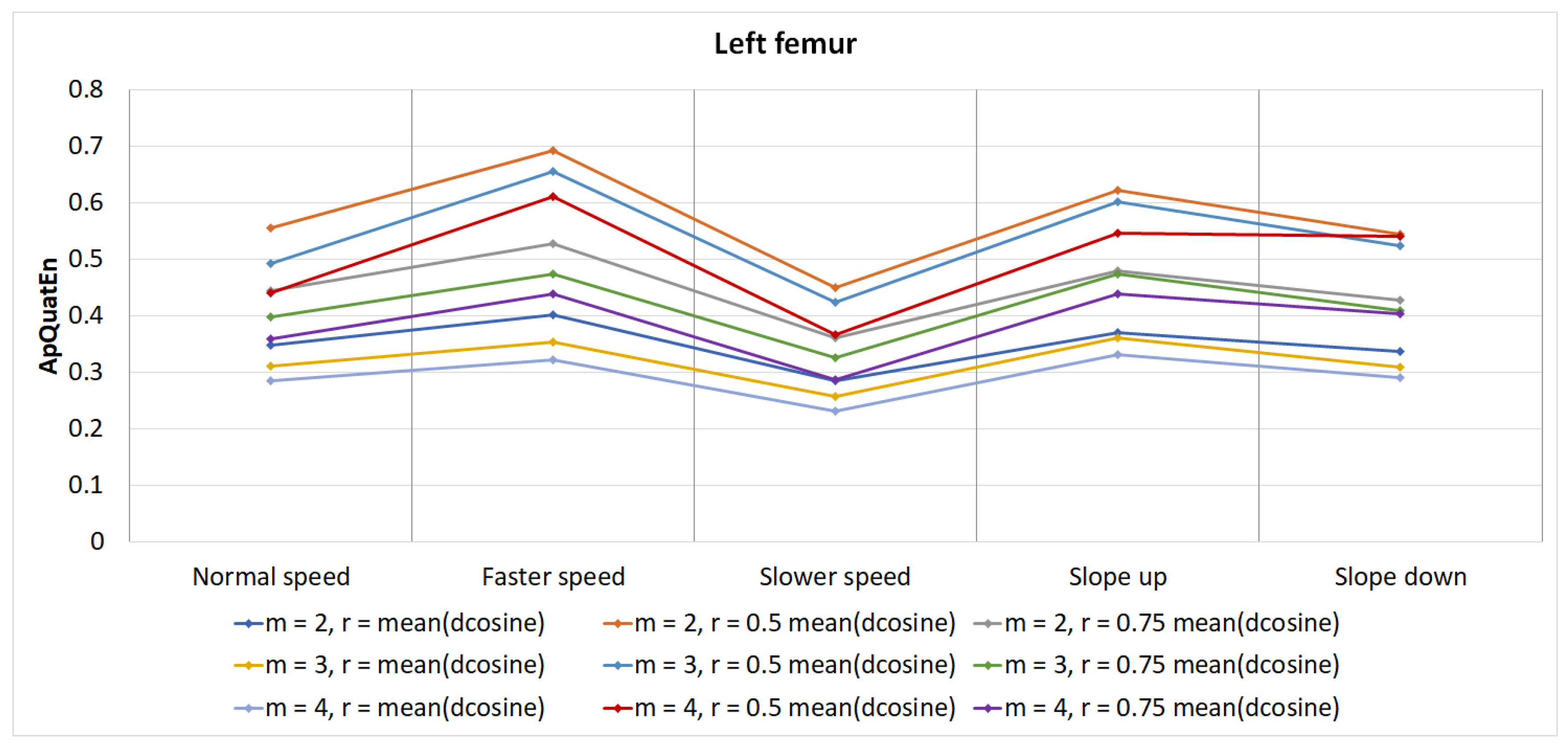
The detailed influence of lengths of vector m and value of threshold r into result for left femur segments is presented in Figure 5. All values of entropy have similar dependencies within experiment configurations and segments. Generally, the for is smaller than for . This means that differences between and are smaller than and . Typically, it is suggested that, for clinical data, m is to be set at 2 when utilizing the algorithm [7].
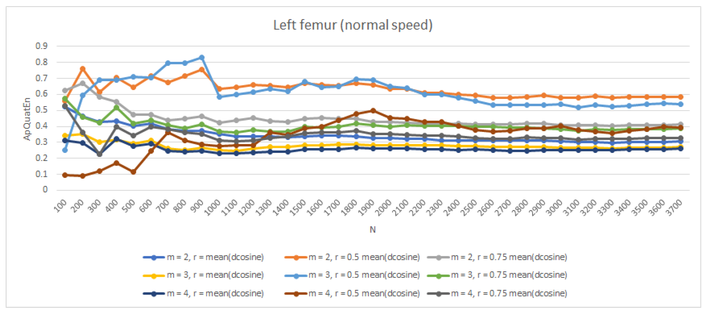
In [14], values were quantified on generated data from 100 to 10,000 data points, in increments of 100. As can be seen, the entropy values stabilize around N of 2000. In order to check the stabilization of entropy values as N increased in experiment data, the chaotic logistic map was subjected to entropy analysis up to an N of 3700 data points. For this particular analysis, (, ) was chosen. Entropy was quantified on data in increments of 100. As can be seen in Figure 6, the entropy values stabilize around an N of 2700 time samples. For gait with Normal velocity, this is after a twenty-second stride.
4. Conclusions
This publication concerns the new quaternion approximate entropy for quaternion time series represented orientations of human skeleton segments. The presented approach was used to quantify chaotic behavior in the context of regularity in time series. The example of application for treadmill walking data, in five variants of walking speed and treadmill slope, was discussed. Data was obtained from the optical motion capture system. It was confirmed that all considered time series are characterized by positive values of entropy values which quantify a local instability. The use of entropy as a mathematical tool to quantify predictability of gait parameters is an entirely emerging task in human movement research. This is the first proposition to consider quaternion signal and has analysed the correlated data which describe rotation in 3D. A possible future work can be related to develop quaternion version of negentropies to develop hypothesis testing for normality [32].
Funding
This publication was supported by the Rector’s grant in the field of scientific research and development works, Silesian University of Technology (Gliwice, Poland), Grant No. 02/020/RGJ/18/0125, (2018–2019).
Acknowledgments
The data was captured in the Human Motion Lab (HML) of the Polish-Japanese Academy of Information Technology in Bytom, Poland (http://bytom.pja.edu.pl/).
Conflicts of Interest
The author declares no conflict of interest.
References
- Schuster, H.G.; Just, W. Deterministic Chaos: An Introduction; John Wiley & Sons: New York, NY, USA, 2006. [Google Scholar]
- Wolf, A.; Swift, J.B.; Swinney, H.L.; Vastano, J.A. Determining Lyapunov exponents from a time series. Phys. D Nonlinear Phenom. 1985, 16, 285–317. [Google Scholar] [CrossRef] [Green Version]
- Pincus, S. Approximate entropy (ApEn) as a complexity measure. Chaos Interdiscip. J. Nonlinear Sci. 1995, 5, 110–117. [Google Scholar] [CrossRef]
- Pincus, S.M. Approximate entropy as a measure of system complexity. Proc. Natl. Acad. Sci. USA 1991, 88, 2297–2301. [Google Scholar] [CrossRef] [PubMed]
- Eckmann, J.P.; Ruelle, D. Ergodic theory of chaos and strange attractors. In The Theory of Chaotic Attractors; Springer: Berlin/Heidelberg, Germany, 1985; pp. 273–312. [Google Scholar]
- Richman, J.S.; Moorman, J.R. Physiological time-series analysis using approximate entropy and sample entropy. Am. J. Physiol.-Heart Circ. Physiol. 2000, 278, H2039–H2049. [Google Scholar] [CrossRef] [PubMed]
- Pincus, S.M.; Viscarello, R.R. Approximate entropy: A regularity measure for fetal heart rate analysis. Obstet Gynecol 1992, 79, 249–255. [Google Scholar] [PubMed]
- Kaplan, D.; Furman, M.; Pincus, S.; Ryan, S.; Lipsitz, L.; Goldberger, A. Aging and the complexity of cardiovascular dynamics. Biophys. J. 1991, 59, 945. [Google Scholar] [CrossRef]
- Liu, C.; Liu, C.; Shao, P.; Li, L.; Sun, X.; Wang, X.; Liu, F. Comparison of different threshold values r for approximate entropy: Application to investigate the heart rate variability between heart failure and healthy control groups. Physiol. Meas. 2010, 32, 167. [Google Scholar] [CrossRef] [PubMed]
- Abásolo, D.; Hornero, R.; Espino, P.; Poza, J.; Sánchez, C.I.; de la Rosa, R. Analysis of regularity in the EEG background activity of Alzheimer’s disease patients with Approximate Entropy. Clin. Neurophysiol. 2005, 116, 1826–1834. [Google Scholar] [CrossRef] [PubMed]
- Zhang, X.S.; Roy, R.J.; Jensen, E.W. EEG complexity as a measure of depth of anesthesia for patients. IEEE Trans. Biomed. Eng. 2001, 48, 1424–1433. [Google Scholar] [CrossRef] [PubMed]
- Kannathal, N.; Choo, M.L.; Acharya, U.R.; Sadasivan, P. Entropies for detection of epilepsy in EEG. Comput. Methods Progr. Biomed. 2005, 80, 187–194. [Google Scholar] [CrossRef] [PubMed]
- Acharya, U.R.; Molinari, F.; Sree, S.V.; Chattopadhyay, S.; Ng, K.H.; Suri, J.S. Automated diagnosis of epileptic EEG using entropies. Biomed. Signal Process. Control 2012, 7, 401–408. [Google Scholar] [CrossRef]
- Yentes, J.M.; Hunt, N.; Schmid, K.K.; Kaipust, J.P.; McGrath, D.; Stergiou, N. The appropriate use of approximate entropy and sample entropy with short data sets. Ann. Biomed. Eng. 2013, 41, 349–365. [Google Scholar] [CrossRef] [PubMed]
- Costa, M.; Peng, C.K.; Goldberger, A.L.; Hausdorff, J.M. Multiscale entropy analysis of human gait dynamics. Phys. A Stat. Mech. Its Appl. 2003, 330, 53–60. [Google Scholar] [CrossRef]
- Ahmadi, S.; Sepehri, N.; Wu, C.; Szturm, T. Sample Entropy of Human Gait Center of Pressure Displacement: A Systematic Methodological Analysis. Entropy 2018, 20, 579. [Google Scholar] [CrossRef]
- Ramdani, S.; Seigle, B.; Lagarde, J.; Bouchara, F.; Bernard, P.L. On the use of sample entropy to analyze human postural sway data. Med. Eng. Phys. 2009, 31, 1023–1031. [Google Scholar] [CrossRef] [PubMed]
- Bisi, M.; Stagni, R. Complexity of human gait pattern at different ages assessed using multiscale entropy: From development to decline. Gait Posture 2016, 47, 37–42. [Google Scholar] [CrossRef] [PubMed]
- Costa, M.; Goldberger, A.L.; Peng, C.K. Multiscale entropy analysis of biological signals. Phys. Rev. E 2005, 71, 021906. [Google Scholar] [CrossRef] [PubMed]
- McGregor, S.J.; Busa, M.A.; Skufca, J.; Yaggie, J.A.; Bollt, E.M. Control entropy identifies differential changes in complexity of walking and running gait patterns with increasing speed in highly trained runners. Chaos Interdiscip. J. Nonlinear Sci. 2009, 19, 026109. [Google Scholar] [CrossRef]
- Szczęsna, A.; Świtoński, A.; Słupik, J.; Josiński, H.; Wojciechowski, K. Wavelet features in motion data classification. In Proceedings of the International Conference on Numerical Analysis and Applied Mathematics 2015 (ICNAAM-2015), Rhodes, Greece, 23–29 September 2015; AIP Publishing: Melville, NY, USA, 2016; Volume 1738. [Google Scholar]
- Piórek, M.; Josiński, H.; Michalczuk, A.; Świtoński, A.; Szczęsna, A. Quaternions and joint angles in an analysis of local stability of gait for different variants of walking speed and treadmill slope. Inf. Sci. 2017, 384, 263–280. [Google Scholar] [CrossRef]
- Szczęsna, A. Verification of the blobby quaternion model of human joint limits. Biomed. Signal Process. Control 2018, 39, 130–138. [Google Scholar] [CrossRef]
- Szczęsna, A. Quaternion wavelet-based energy and entropy to analysis human gait data. In Proceedings of the International Conference on Numerical Analysis and Applied Mathematics 2017 (ICNAAM-2017), Thessaloniki, Greece, 25–30 September 2017; AIP Publishing: Melville, NY, USA, 2018; Volume 1978. [Google Scholar]
- Szczęsna, A.; Świtoński, A.; Słupik, J.; Zghidi, H.; Josiński, H.; Wojciechowski, K. Quaternion Lifting Scheme Applied to the Classification of Motion Data. Inf. Sci. 2018. [Google Scholar] [CrossRef]
- Switonski, A.; Josinski, H.; Wojciechowski, K. Dynamic time warping in classification and selection of motion capture data. Multidimens. Syst. Signal Process. 2018. [Google Scholar] [CrossRef]
- Hanson, A.J. Visualizing Quaternions; Morgan Kaufmann: Burlington, MA, USA, 2005. [Google Scholar]
- Goldman, R. Understanding quaternions. Gr. Models 2011, 73, 21–49. [Google Scholar] [CrossRef]
- Huynh, D.Q. Metrics for 3D rotations: Comparison and analysis. J. Math. Imaging Vis. 2009, 35, 155–164. [Google Scholar] [CrossRef]
- Gramkow, C. On averaging rotations. J. Math. Imaging Vis. 2001, 15, 7–16. [Google Scholar] [CrossRef]
- Josiński, H.; Michalczuk, A.; Świtoński, A.; Mucha, R.; Wojciechowski, K. Quantifying chaotic behavior in treadmill walking. In Proceedings of the Asian Conference on Intelligent Information and Database Systems, Bali, Indonesia, 23–25 March 2015; pp. 317–326. [Google Scholar]
- Arellano-Valle, R.B.; Contreras-Reyes, J.E.; Stehlík, M. Generalized skew-normal negentropy and its application to fish condition factor time series. Entropy 2017, 19, 528. [Google Scholar] [CrossRef]
Figure 1.
Axis and angle of rotation of femur and foot segments during gait (three strides).

Figure 2.
Results values of (, ) for left and right femur segments.

Figure 3.
Results values of (, ) for left and right tibia segments.

Figure 4.
Results values of (, ) for left and right foot segments.

Figure 5.
The value of entropy in relation to the length of vector (m) and threshold distance r value for left femur segments.
Figure 5.
The value of entropy in relation to the length of vector (m) and threshold distance r value for left femur segments.

Figure 6.
The value of entropy for left femur segments (Normal speed) (, ) in relation to data length N.
Figure 6.
The value of entropy for left femur segments (Normal speed) (, ) in relation to data length N.


Table 1.
Median values of (, ).
| Normal | Faster | Slower | Up | Down | |
|---|---|---|---|---|---|
| lfemur | 0.334 | 0.371 | 0.274 | 0.405 | 0.344 |
| rfemur | 0.345 | 0.406 | 0.300 | 0.371 | 0.396 |
| femur | 0.337 | 0.388 | 0.286 | 0.387 | 0.371 |
| ltibia | 0.252 | 0.446 | 0.138 | 0.599 | 0.353 |
| rtibia | 0.554 | 0.519 | 0.570 | 0.463 | 0.396 |
| tibia | 0.338 | 0.519 | 0.233 | 0.537 | 0.385 |
| lfoot | 0.478 | 0.525 | 0.496 | 0.467 | 0.529 |
| rfoot | 0.420 | 0.552 | 0.356 | 0.447 | 0.396 |
| foot | 0.443 | 0.544 | 0.410 | 0.447 | 0.447 |
Table 2.
The Pearson correlation coefficient of (, ) calculated for left and right femur segments.
| Left Femur | Right Femur | ||||||||||
|---|---|---|---|---|---|---|---|---|---|---|---|
| Normal | Faster | Slower | Up | Down | Normal | Faster | Slower | Up | Down | ||
| Normal | 1.000 | 0.699 | 0.378 | 0.157 | 0.334 | Normal | 1.000 | 0.862 | 0.412 | 0.347 | 0.343 |
| Faster | 0.699 | 1.000 | 0.462 | 0.303 | 0.476 | Faster | 0.862 | 1.000 | 0.699 | 0.537 | 0.604 |
| Slower | 0.378 | 0.462 | 1.000 | 0.921 | 0.941 | Slower | 0.412 | 0.699 | 1.000 | 0.899 | 0.951 |
| Up | 0.157 | 0.303 | 0.921 | 1.000 | 0.944 | Up | 0.347 | 0.537 | 0.899 | 1.000 | 0.834 |
| Down | 0.334 | 0.476 | 0.940 | 0.944 | 1.000 | Down | 0.343 | 0.604 | 0.951 | 0.834 | 1.000 |
Table 3.
The Pearson correlation coefficient of (, ) calculated for left and right tibia segments.
| Left Tibia | Right Tibia | ||||||||||
|---|---|---|---|---|---|---|---|---|---|---|---|
| Normal | Faster | Slower | Up | Down | Normal | Faster | Slower | Up | Down | ||
| Normal | 1.000 | 0.695 | 0.733 | 0.143 | 0.564 | Normal | 1.000 | 0.611 | 0.718 | 0.874 | 0.458 |
| Faster | 0.695 | 1.000 | 0.632 | 0.328 | 0.549 | Faster | 0.611 | 1.000 | 0.505 | 0.496 | 0.439 |
| Slower | 0.733 | 0.632 | 1.000 | 0.409 | 0.744 | Slower | 0.718 | 0.505 | 1.000 | 0.797 | 0.685 |
| Up | 0.143 | 0.328 | 0.409 | 1.000 | 0.542 | Up | 0.874 | 0.496 | 0.797 | 1.000 | 0.646 |
| Down | 0.564 | 0.549 | 0.744 | 0.542 | 1.000 | Down | 0.458 | 0.439 | 0.685 | 0.646 | 1.000 |
Table 4.
The Pearson correlation coefficient of (, ) calculated for left and right foot segments.
| Left Foot | Right Foot | ||||||||||
|---|---|---|---|---|---|---|---|---|---|---|---|
| Normal | Faster | Slower | Up | Down | Normal | Faster | Slower | Up | Down | ||
| Normal | 1.000 | 0.728 | 0.510 | 0.439 | 0.491 | Normal | 1.000 | 0.721 | 0.491 | 0.135 | 0.390 |
| Faster | 0.728 | 1.000 | 0.778 | 0.573 | 0.773 | Faster | 0.721 | 1.000 | 0.449 | 0.241 | 0.237 |
| Slower | 0.510 | 0.778 | 1.000 | 0.837 | 0.923 | Slower | 0.491 | 0.449 | 1.000 | 0.901 | 0.909 |
| Up | 0.439 | 0.573 | 0.837 | 1.000 | 0.751 | Up | 0.135 | 0.241 | 0.901 | 1.000 | 0.841 |
| Down | 0.491 | 0.773 | 0.923 | 0.751 | 1.000 | Down | 0.390 | 0.237 | 0.909 | 0.841 | 1.000 |
© 2019 by the author. Licensee MDPI, Basel, Switzerland. This article is an open access article distributed under the terms and conditions of the Creative Commons Attribution (CC BY) license (http://creativecommons.org/licenses/by/4.0/).
Share and Cite
MDPI and ACS Style
Szczęsna, A. Quaternion Entropy for Analysis of Gait Data. Entropy 2019, 21, 79. https://doi.org/10.3390/e21010079
AMA Style
Szczęsna A. Quaternion Entropy for Analysis of Gait Data. Entropy. 2019; 21(1):79. https://doi.org/10.3390/e21010079
Chicago/Turabian StyleSzczęsna, Agnieszka. 2019. "Quaternion Entropy for Analysis of Gait Data" Entropy 21, no. 1: 79. https://doi.org/10.3390/e21010079
Note that from the first issue of 2016, this journal uses article numbers instead of page numbers. See further details here.