Information Entropy of Tight-Binding Random Networks with Losses and Gain: Scaling and Universality


Instituto de Física, Benemérita Universidad Autónoma de Puebla, Apartado Postal J-48, Puebla 72570, Mexico
*
Author to whom correspondence should be addressed.
Entropy 2019, 21(1), 86; https://doi.org/10.3390/e21010086
Submission received: 12 October 2018
/
Revised: 1 January 2019
/
Accepted: 15 January 2019
/
Published: 18 January 2019
(This article belongs to the Special Issue Complex Networks from Information Measures)
Abstract
:We study the localization properties of the eigenvectors, characterized by their information entropy, of tight-binding random networks with balanced losses and gain. The random network model, which is based on Erdős–Rényi (ER) graphs, is defined by three parameters: the network size N, the network connectivity , and the losses-and-gain strength . Here, N and are the standard parameters of ER graphs, while we introduce losses and gain by including complex self-loops on all vertices with the imaginary amplitude i with random balanced signs, thus breaking the Hermiticity of the corresponding adjacency matrices and inducing complex spectra. By the use of extensive numerical simulations, we define a scaling parameter that fixes the localization properties of the eigenvectors of our random network model; such that, when (), the eigenvectors are localized (extended), while the localization-to-delocalization transition occurs for . Moreover, to extend the applicability of our findings, we demonstrate that for fixed , the spectral properties (characterized by the position of the eigenvalues on the complex plane) of our network model are also universal; i.e., they do not depend on the specific values of the network parameters.
1. Introduction
Independently of the field, classification, or application, a commonly-accepted mathematical representation of a network or graph is the adjacency matrix. The adjacency matrix of a simple non-directed network (a simple network is a network not having multiple edges or self-edges) is the matrix with elements defined as [1]:
This prescription produces symmetric sparse matrices with zero diagonal elements, where N is the number of vertices of the corresponding network. The sparsity of is quantified by the parameter , which is the fraction of non-vanishing off-diagonal adjacency matrix elements. Vertices are isolated when , whereas the network is fully connected for . Once the adjacency matrix of a network is constructed, it is quite natural to ask about the properties of its eigenvalues and eigenvectors, which is the main subject of this paper. As commonly used, we refer to the properties of the eigenvalues and eigenvectors of the adjacency matrix as the properties of the eigenvalues and eigenvectors of the respective network.
1.1. Network Model with Losses and Gain
First, we want to recall that there is a one-to-one correspondence between the adjacency matrix of Equation (1) and the Hamiltonian matrix of a -dimensional solid, described by Anderson’s tight-binding model [2] with zero on-site potentials () and constant hopping integrals (). Here, is proportional to the average non-zero off-diagonal adjacency matrix elements per matrix row and, therefore, may be regarded as the effective dimension of a tight-binding random network represented by , as discussed in [3] from a Random Matrix Theory (RMT) point of view. This correspondence enables the direct application of studies originally motivated by physical systems, represented by sparse random Hamiltonian matrices, to complex networks. Tight-binding models are widely used in solid state physics to study the electronic properties of systems composed by atoms (molecules, potentials, or sites; in more general terms) whose electrons are tightly bound to the atoms they belong to, so they have limited interaction with neighbor atoms; see, e.g., [4]. Moreover, recently, tight-binding models have also been studied on random and regular graphs; see some examples in [5,6,7,8,9,10,11,12,13].
The tight-binding random network model we shall use in our study is defined as follows. Starting with the standard Erdős–Rényi (ER) network, we add to it self-edges and further consider all edges to have random strengths. Our main motivation to include weights, particularly random weights, in the standard ER model is to retrieve well-known random matrices in the appropriate limits in order to use RMT results as a reference (see below). Moreover, we would like to note that in realistic graphs, vertices and edges may not be equivalent (i.e., the graph might be composed of different agents, where different pairs interact with different intensities); therefore, their corresponding adjacency matrices are not just binary. In this sense, random weights can be considered as a limit case where all vertices and edges in a graph are different. Indeed, random weights have been used in other complex network models; see some examples in [14,15]. We have named this model as the ER fully-random network model [5,16,17]. The sparsity is defined as the fraction of the independent non-vanishing off-diagonal adjacency matrix elements. Then, as in the standard ER model, the ER fully-random network model (whose adjacency matrices come from the ensemble of sparse real symmetric matrices) is characterized by the parameters N and . In this study, we add the imaginary amplitude ±i to the self-edge weights of the ER fully-random network model such that the corresponding adjacency matrices are defined as:
Here, are statistically-independent random variables drawn from a normal distribution with zero mean and variance one. Note that the term , with , makes the adjacency matrix of the tight-binding random network model non-Hermitian, which, in turn, has complex eigenvalues and eigenvectors. According to this definition, a diagonal random matrix is obtained for and = 0 (Poisson case), whereas the Gaussian Orthogonal Ensemble (GOE) is recovered when and . The GOE is a random matrix ensemble formed by real symmetric random matrices whose entries are statistically-independent random variables drawn from a normal distribution with zero mean and variance ; see, e.g., [18]. The GOE is commonly used to statistically represent Hamiltonian matrices corresponding to complex, chaotic, or disordered systems having time-reversal invariance.
The random network model with the adjacency matrix of Equation (2) is inspired by non-Hermitian Hamiltonians describing open or scattering systems, systems interacting with an environment, or active materials. Within the effective non-Hermitian Hamiltonian approach, such opening or interaction is modeled by adding complex terms to the main diagonal of the Hamiltonian of the system of interest [19,20,21,22,23]. Indeed, in tight-binding systems, the on-site term represents losses () and gain (). Moreover, the term allows adding losses and gain to tight-binding systems locally by adding this term to selected sites (in regular arrays, the addition of the term to border sites is commonly used to study scattering and transport properties; see, e.g., [24,25,26]), globally by adding this term to all sites in the system (in linear chains, the addition of the term to all sites has been used to represent a system coupled to a common decay channel; see, e.g., [27,28]), and in a balanced way by adding to all sites with the same proportion of plus and minus signs (the addition of alternating and terms to the sites of one-dimensional non-disordered arrays produces -symmetric wires; see, e.g., [29,30]). In our model, we choose the latter setup, where balanced implies that the network is formed by an even number of vertices. Our main motivation to choose a balanced loss-and-gain setup is to limit the number of parameters of the model, since a non-balanced setup would require including the loss-to-gain ratio as a parameter. Furthermore, since the vertices of our network are not ordered, the balanced loss and gain is effectively introduced randomly to the network. This is in contrast to -symmetric systems [29], where loss and gain alternate periodically. Thus, in our model, is the loss-and-gain strength.
Therefore, our random network model corresponds to tight-binding random networks with random on-site potentials, random hopping integrals, and random on-site loss and gain. Our random network model depends on three parameters: the network size N, the network connectivity , and the losses-and-gain strength .
1.2. Previous Work
As precedents, we can mention that we have already studied some spectral [16,17], eigenvector [16], and transport [5] properties of ER-type random networks with a special focus on universality, from a random matrix theory (RMT) point of view. Moreover, we have also performed scaling studies on other random networks models, such as multilayer and multiplex networks [15,31] and random-geometric and random-rectangular graphs [32]. In particular, for ER fully-random networks, we have shown that [16] the average information entropy (to be defined below) is a function of the average degree . Moreover, describes the delocalization transition of the network model well: (i) for , where , the eigenvectors are practically localized; hence, the delocalization transition takes place around (for which becomes larger than zero, meaning that the corresponding eigenvectors have more than only one principal component), which is close to previous theoretical and numerical estimations [33,34,35,36]; and (ii) for , where , the eigenvectors are practically random and fully extended. Here, is the entropy of the eigenvectors of the GOE, i.e., random eigenvectors with Gaussian-distributed amplitudes. Thus, the study of [16] provides a tool to predict the localization properties of the eigenvectors of ER-type random networks once the parameter is known.
2. Results
2.1. Scaling of Information Entropy
In order to characterize quantitatively the complexity, and in specific cases the fractality, of the normalized eigenvectors of random matrices (and of Hamiltonians corresponding to disordered and quantized chaotic systems), the Rényi entropies are widely used:
Here, the subindex n refers to the eigenvector component, and form the discrete probability distribution associated with the eigenvector (where stands for the modulus of a complex number); with and . In our study, we use the information entropy (given by Equation (3) in the limit ):
Note that the minimal value of S, , is obtained when only one component in the eigenvector concentrates all the probability; while the maximal value of S, , is approached when the probability is evenly distributed over the eigenvector: for all n. Any other possible configuration of probabilities , including the eigenvectors of the GOE, provides . Therefore, the exponential of S is known to be a good measure of eigenvector localization [47], since it provides the number of principal components of an eigenvector in a given basis. That is, when S = 0, the eigenvector has only one principal component, , so it is localized; while it is fully extended, , when . Here, we refer to the principal components of an eigenvector as the eigenvector components having the largest amplitudes. In fact, S has been already used to characterize the eigenvectors of adjacency matrices of several random network models (see some examples in [15,16,48,49,50,51]).
With Definition (4), when for any , since the eigenvectors of the (diagonal) adjacency matrices of our random network model have only one non-vanishing component with the magnitude equal to one, then . On the other hand, for and , the GOE is reproduced, and ; i.e., the random eigenvectors extend over the N available vertices in the network. We note that for and , our random network model does not reproduce the GOE and ; however, we observe that , so we use as the reference information entropy.
Below, we use exact numerical diagonalization to obtain the eigenvectors and eigenvalues () of the adjacency matrices of large ensembles of tight-binding random networks characterized by N, , and . Then, we average over all eigenvectors of an ensemble of adjacency matrices of size N to compute . We have verified that our conclusions are not modified when we restrict the averages to a fraction of the eigenvectors around the band center, which is a prescription commonly used in RMT studies.
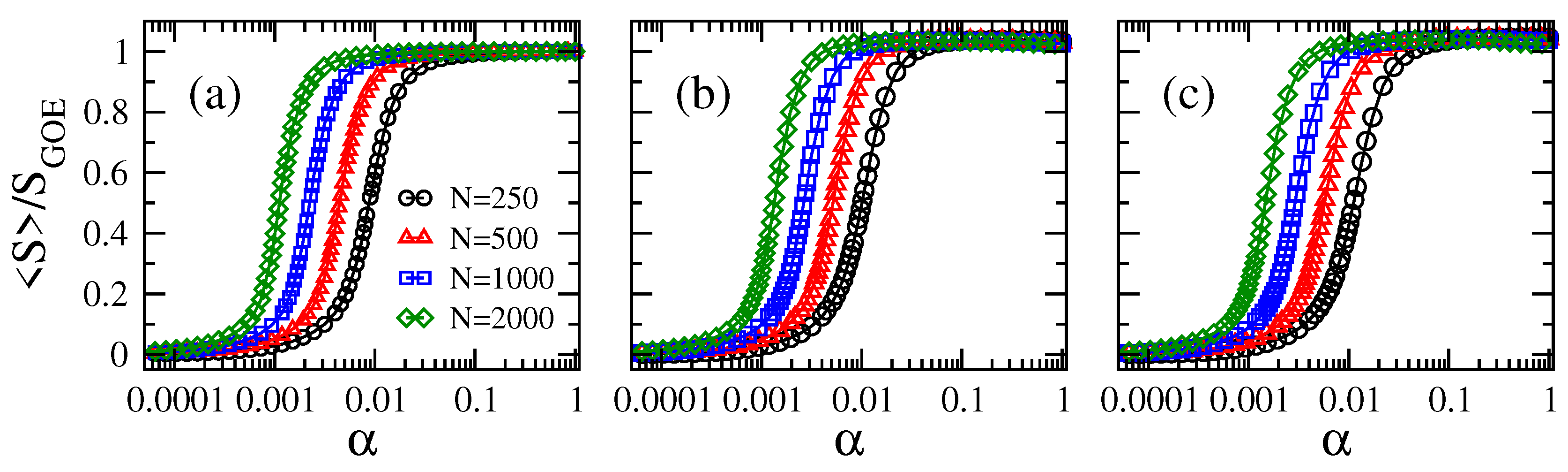
In Figure 1 and Figure 2, we show the average information entropy , normalized to , as a function of the connectivity for the adjacency matrices of ER tight-binding random networks with balanced losses and gain. We observe that the curves of , for any combination of N and , have a very similar functional form as a function of : the curves show a smooth transition from approximately zero (localized regime) to approximately one (delocalized regime) when increases from (mostly isolated vertices) to one (fully-connected graphs).
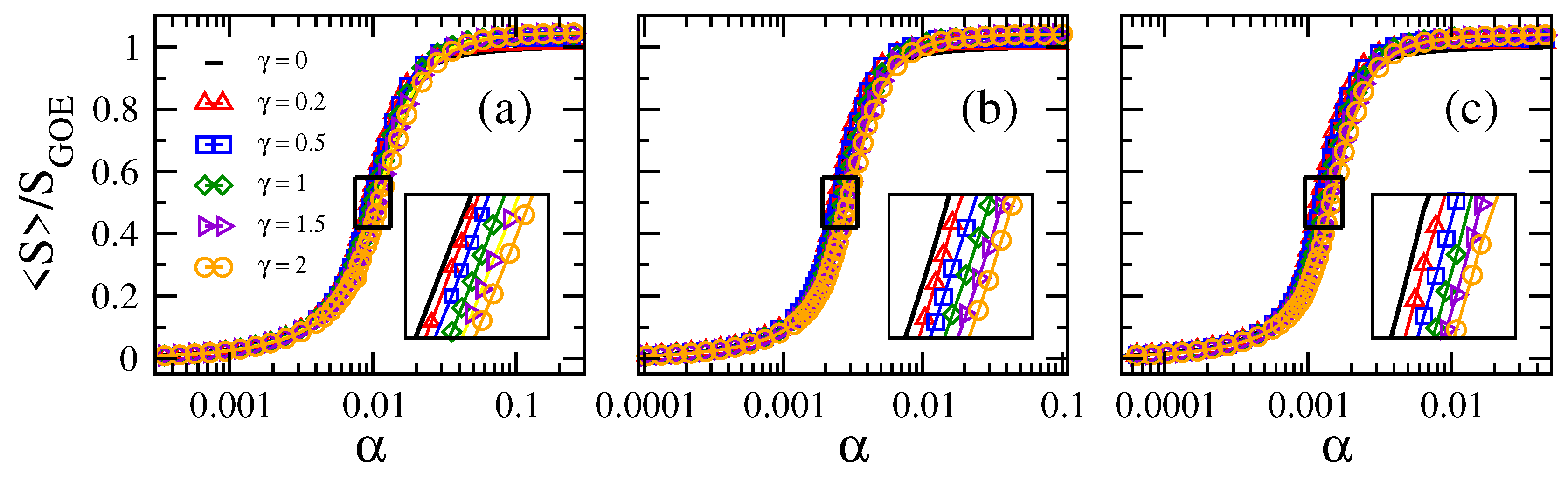
From Figure 1, for fixed , we observe that the larger the network size N, the smaller the value of needed to approach the delocalized regime. Furthermore, note that the curves of vs. are shifted to the left on the -axis for increasing N. All this panorama is in accordance with the case , as shown in [16]. In contrast, for fixed N, the curves of vs. are displaced to the right on the -axis for increasing ; clearly seen in the insets of Figure 2. As a reference, we include the case as black full lines in all panels of Figure 2. Moreover, the fact that these curves, plotted in semi-log scale, are just shifted on the -axis when tuning N or makes us forecast the existence of a scaling parameter that depends on both N and . In order to look for the scaling parameter, we first define a quantity to characterize the position of the curves on the -axis: indeed, we choose the value of , which we label as , for which . Notice that characterizes the localization-to-delocalization transition of the eigenvectors of our network model.
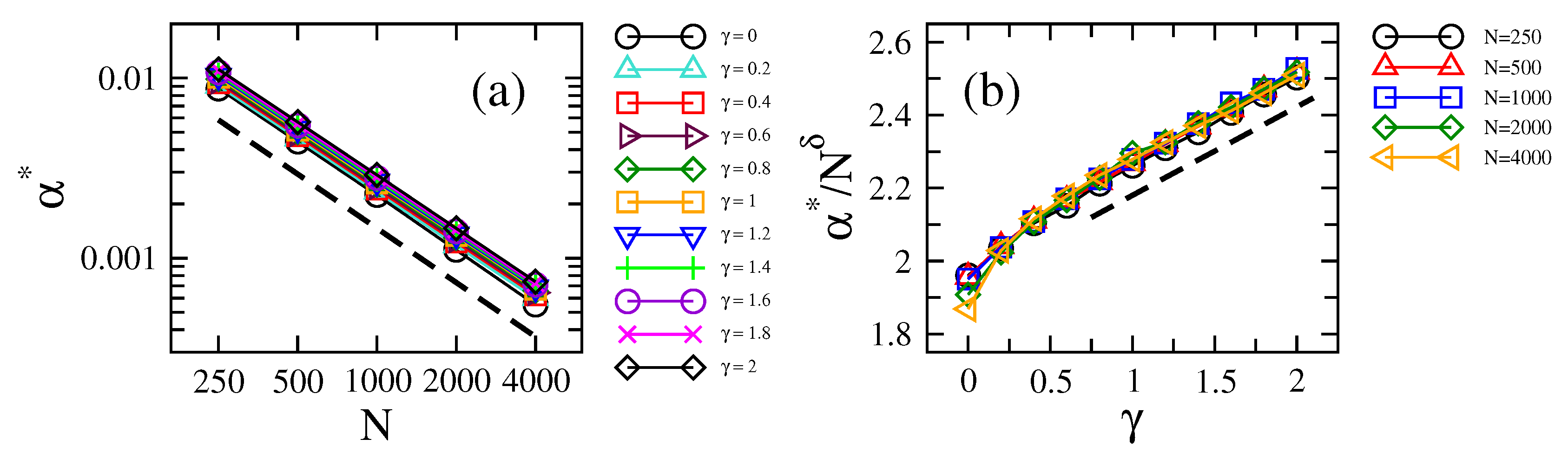
Then, in Figure 3a,b, we present the localization-to-delocalization transition point as a function of N and , respectively. On the one hand, the linear trend of the data (in log-log scale) in Figure 3a implies a power-law relation of the form:
In fact, Equation (5) provides very good fittings to the data (the values of the fitting parameters are reported in Table 1). Note that for all , a slight difference with the case where ; see also [16]. On the other hand, in Figure 3b, we plot the ratio , with , as a function of . With this, we already take into account the scaling stated in Equation (5), which, at the same time, allows us to examine the dependence of on more easily. Indeed, for , we conclude that:
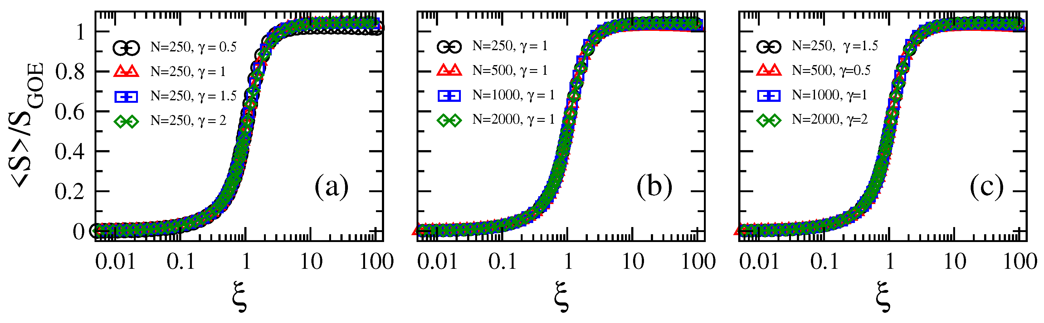
Therefore, by plotting again the curves of now as a function of the connectivity divided by the localization-to-delocalization transition point,
we observe that curves for different parameter combinations collapse on top of a universal curve; i.e., a curve that depends on the parameter only; see Figure 4. This means that once the ratio is fixed, no matter the graph size and the loss-and-gain strength, the information entropy of the eigenvectors is also fixed.
2.2. Eigenvalue Properties
Once we have found that (see Equations (6) and (7)) is the parameter that scales the eigenvector properties (characterized by their information entropy) of our model of random networks with losses and gain, we believe that other properties (i.e., spectral properties) of the network model may also be scaled by the same parameter. Thus, in the following, we validate our surmise by analyzing the corresponding eigenvalues.
Recall that for , the adjacency matrices of our random network model are Hermitian and the corresponding spectra are real. For any , the adjacency matrices become non-Hermitian and their eigenvalues are complex numbers.
Now, in Figure 5, we show density plots (in the complex plane) of the eigenvalues of Erdős–Rényi tight-binding random networks with losses and gain for several parameter combinations. In this figure, we can clearly see the competition of the two main parameters of the model: the sparsity and the loss-and-gain strength (for fixed N). On the one side, for small (i.e., mostly isolated vertices), the main diagonal of the adjacency matrices dominates and the imaginary part of the corresponding eigenvalues is approximately equal to ; see Figure 5 (left panels). That is, the eigenvalues form two thin clouds around . On the other side, for large (i.e., highly-connected graphs), the density of off-diagonal elements of the adjacency matrices is also large, and the corresponding eigenvalues form a cloud with center at the origin of the complex plane that gets wider for increasing ; see Figure 5 (right panels) with . Moreover, for , this cloud splits into two clouds that separate further from the real axis for even larger values of ; see Figure 5 (right panels) with . It is remarkable that the cloud splits for , since it corresponds to the super-radiance transition value reported for full random matrices [52], one-dimensional disordered tight-binding wires [26,27,53,54,55], and random many-body systems [56].
The super-radiance transition is a phase transition that occurs, as a function of the coupling strength, in quantum systems coupled to common decay channels; see, e.g., [20,21,22,23,57]. It was originally predicted by the Dicke model of super-radiance [58]. In very general terms, this transition occurs at a given coupling strength above which a number of internal states (eigenvalues) acquire decay widths (imaginary part of the eigenvalues) proportional to the coupling strength. Thus, even though a more detailed analysis is necessary, we can assume that the splitting of the density plots of eigenvalues in the complex plane at (as observed in Figure 5) is a signature of the super-radiance transition in our tight-binding random network model.
Finally, for moderate values of , as reported in Figure 5 (central panels), the combination of the two situations described above occurs: for small , the eigenvalues form three clouds in the complex plane, two thin ones close to , and a third one with the center at the origin of the complex plane; for increasing , the middle cloud gets wider and splits into two clouds that, for large enough , merge with the thin clouds at .
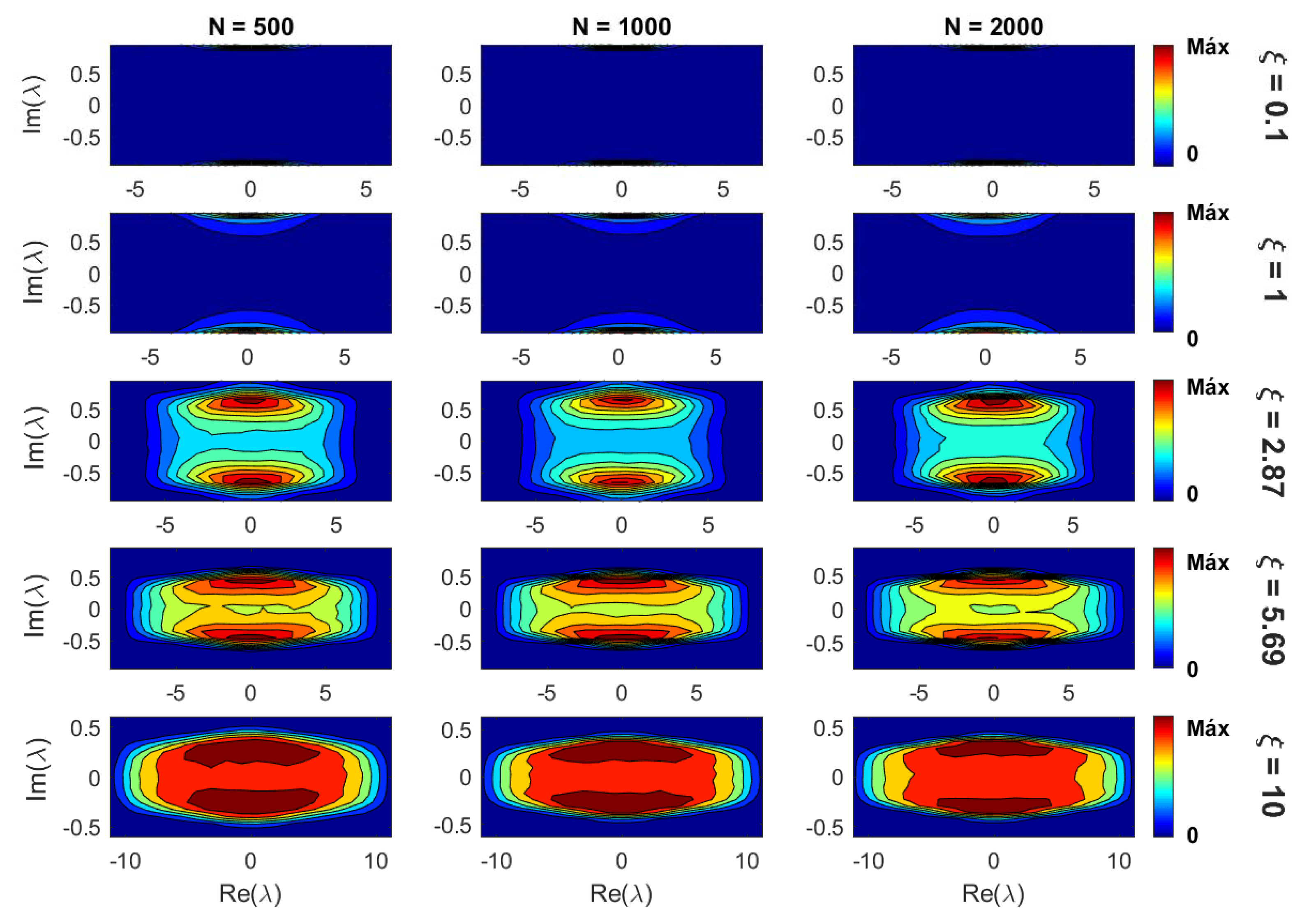
Notice that the panorama shown in Figure 5 (where networks of size were used), even though it is valid for any N, will be shifted for different network sizes; as can be inferred from the information entropy of the eigenvectors reported in Figure 1. Moreover, the scaling analysis made in the previous subsection allowed us to define the scaling parameter that fixes the eigenvector properties of our random network model, as shown in Figure 4. Therefore, in Figure 6 we present density plots of eigenvalues for three network sizes and increasing values of (from top to bottom). It is clear from Figure 6 that once is fixed, the density of eigenvalues in the complex plane is (statistically) the same for different parameter combinations. Thus, we validate that the eigenvalue properties of our model are also scaled with the parameter .
3. Summary
In this paper, we have numerically studied the eigenvector and eigenvalue properties of the adjacency matrices of tight-binding random networks with balanced losses and gain. In particular, we focused on scaling and universality from a random matrix theory point of view. We would like to stress that even though we already have some previous experience with scaling studies of random network models (see, e.g., [5,15,16,17,32]), this is the first time we apply this technique to non-Hermitian adjacency matrices.
Specifically, we have considered Erdős–Rényi tight-binding random networks with self-loops (where all non-vanishing adjacency matrix elements are Gaussian random variables) and add the imaginary term to the weights of all vertices to emulate losses () and gain (). We assume balanced losses and gain, so that we include the same number of positive and negative terms . This implies the number of vertices in the network to be an even number. Thus, our random network model depends on three parameters: the network size N, the network connectivity , and the losses-and-gain strength .
First, by the proper scaling analysis of the information entropy of the eigenvectors of the adjacency matrices of our random network model, we obtain , with ; see Equations (6) and (7). Here, is the scaling parameter of the model; that is, for fixed , the information entropy of the eigenvectors is also fixed; see Figure 4. Our analysis provides a way to predict the localization properties of the random networks with losses and gain: for , the eigenvectors are localized; the localization-to-delocalization transition occurs for ; while when , the eigenvectors are extended. Moreover, by recalling that in tight-binding systems, a localization-to-delocalization transition implies an insulator-to-metal transition in the corresponding scattering setup, our results might be used to design the conduction properties of the tight-binding network since tuning N, , and could drive the network from a regime of localized eigenvectors (insulating regime), , to a regime of delocalized eigenvectors (metallic regime), .
Therefore, to extend the applicability of our findings, we demonstrate that for fixed , the spectral properties (characterized by the position of the eigenvalues on the complex plane) of our network model are also universal; i.e., they do not depend on the specific values of the network parameters; see Figure 6.
We expect our results may motivate further numerical, as well as analytical efforts towards the understanding of networks with non-Hermitian adjacency matrices.
Author Contributions
The authors contributed equally to this work. C.T.M.-M. and J.A.M.-B. conceived of, designed, and performed the numerical experiments; C.T.M.-M. and J.A.M.-B. analyzed the data and wrote the paper.
Funding
This work was partially supported by VIEP-BUAP (Grant No. MEBJ-EXC18-G), Fondo Institucional PIFCA (Grant No. BUAP-CA-169), and CONACyT (Grant No. CB-2013/220624).
Conflicts of Interest
The authors declare no conflict of interest. The founding sponsors had no role in the design of the study; in the collection, analyses, or interpretation of data; in the writing of the manuscript; nor in the decision to publish the results.
References
- Newman, M.E.J. Networks: An Introduction; Oxford University Press: New York, NY, USA, 2010. [Google Scholar]
- Anderson, P.W. Absence of diffusion in certain random lattices. Phys. Rev. 1958, 109, 1492–1505. [Google Scholar] [CrossRef]
- Jackson, A.D.; Mejia-Monasterio, C.; Rupp, T.; Saltzer, M.; Wilke, T. Spectral ergodicity and normal modes in ensembles of sparse matrices. Nucl. Phys. A 2001, 687, 405–434. [Google Scholar] [CrossRef] [Green Version]
- Goringe, C.M.; Bowler, D.R.; Hernandez, E. Tight-binding modelling of materials. Rep. Prog. Phys. 1997, 60, 1447–1512. [Google Scholar] [CrossRef]
- Martinez-Mendoza, A.J.; Alcazar-Lopez, A.; Mendez-Bermudez, J.A. Scattering and transport properties of tight-binding random networks. Phys. Rev. E 2013, 88, 122126. [Google Scholar] [CrossRef] [PubMed]
- Biroli, G.; Ribeiro-Teixeira, A.C.; Tarzia, M. Difference between level statistics, ergodicity and localization transitions on the Bethe lattice. arXiv, 2012; arXiv:1211.7334. [Google Scholar]
- De Luca, A.; Altshuler, B.L.; Kravtsov, V.E.; Scardicchio, A. Anderson localization on the Bethe lattice: Nonergodicity of extended states. Phys. Rev. Lett. 2014, 113, 046806. [Google Scholar] [CrossRef] [PubMed]
- Tikhonov, K.S.; Mirlin, A.D.; Skvortsov, M.A. Anderson localization and ergodicity on random regular graphs. Phys. Rev. B 2016, 94, 220203(R). [Google Scholar] [CrossRef]
- Tikhonov, K.S.; Mirlin, A.D. Fractality of wave functions on a Cayley tree: Difference between tree and locally treelike graph without boundary. Phys. Rev. B 2016, 94, 184203. [Google Scholar] [CrossRef]
- Garcia-Mata, I.; Giraud, O.; Georgeot, B.; Martin, J.; Dubertrand, R.; Lemarie, G. Scaling theory of the Anderson transition in random graphs: Ergodicity and universality. Phys. Rev. Lett. 2017, 118, 166801. [Google Scholar] [CrossRef]
- Metz, F.L.; Perez-Castillo, I. Level compressibility for the Anderson model on regular random graphs and the eigenvalue statistics in the extended phase. Phys. Rev. B 2017, 96, 064202. [Google Scholar] [CrossRef]
- Sonner, M.; Tikhonov, K.S.; Mirlin, A.D. Multifractality of wave functions on a Cayley tree: From root to leaves. Phys. Rev. B 2017, 96, 214204. [Google Scholar] [CrossRef] [Green Version]
- Tikhonov, K.S.; Mirlin, A.D. Statistics of eigenstates near the localization transition on random regular graphs. arXiv, 2012; arXiv:1810.11444. [Google Scholar] [CrossRef]
- Jahnke, L.; Kantelhardt, J.W.; Berkovits, R.; Havlin, S. Wave localization in complex networks with high clustering. Phys. Rev. Lett. 2008, 101, 175702. [Google Scholar] [CrossRef] [PubMed]
- Mendez-Bermudez, J.A.; Ferraz-de-Arruda, G.; Rodrigues, F.A.; Moreno, Y. Scaling properties of multilayer random networks. Phys. Rev. E 2017, 96, 012307. [Google Scholar] [CrossRef] [PubMed]
- Mendez-Bermudez, J.A.; Alcazar-Lopez, A.; Martinez-Mendoza, A.J.; Rodrigues, F.A.; Peron, T.K.D.M. Universality in the spectral and eigenvector properties of random networks. Phys. Rev. E 2015, 91, 032122. [Google Scholar] [CrossRef]
- Gera, R.; Alonso, L.; Crawford, B.; House, J.; Mendez-Bermudez, J.A.; Knuth, T.; Miller, R. Identifying network structure similarity using spectral graph theory. Appl. Net. Sci. 2018, 3, 2. [Google Scholar] [CrossRef] [Green Version]
- Metha, M.L. Random Matrices; Elsevier: Amsterdam, The Netherlands, 2004. [Google Scholar]
- Mahaux, C.; Weidenmüller, H.A. Shell Model Approach to Nuclear Reactions; North-Holland: Amsterdam, The Netherlands, 1969. [Google Scholar]
- Sokolov, V.V.; Zelevinsky, V.G. Dynamics and statistics of unstable quantum states. Nucl. Phys. A 1989, 504, 562–588. [Google Scholar] [CrossRef]
- Sokolov, V.V.; Zelevinsky, V.G. On a statistical theory of overlapping resonances. Phys. Lett. B 1988, 202, 10–14. [Google Scholar] [CrossRef]
- Sokolov, V.V.; Zelevinsky, V.G. Collective dynamics of unstable quantum states. Ann. Phys. (N. Y.) 1992, 216, 323–350. [Google Scholar] [CrossRef]
- Rotter, I. A continuum shell model for the open quantum mechanical nuclear system. Rep. Prog. Phys. 1991, 54, 635–682. [Google Scholar] [CrossRef]
- Weiss, M.; Mendez-Bermudez, J.A.; Kottos, T. Resonance width distribution for high dimensional random media. Phys. Rev. B 2006, 73, 045103. [Google Scholar] [CrossRef]
- Herrera-Gonzalez, I.F.; Mendez-Bermudez, J.A.; Izrailev, F.M. Transport through quasi-one-dimensional wires with correlated disorder. Phys. Rev. E 2014, 90, 042115. [Google Scholar] [CrossRef] [PubMed]
- Herrera-Gonzalez, I.F.; Mendez-Bermudez, J.A.; Izrailev, F.M. Distribution of S-matrix poles for one-dimensional disordered wires. arXiv, 2016; arXiv:1810.06166. [Google Scholar]
- Celardo, G.L.; Biella, A.; Kaplan, L.; Borgonovi, F. Interplay of superradiance and disorder in the Anderson Model. Fortschr. Phys. 2013, 61, 250. [Google Scholar] [CrossRef]
- Chavez, N.C.; Mattiotti, F.; Mendez-Bermudez, J.A.; Borgonovi, F.; Celardo, G.L. Real and imaginary energy gaps: A comparison between single excitation Superradiance and Superconductivity. arXiv, 2018; arXiv:1805.03153. [Google Scholar]
- El-Ganainy, R.; Makris, K.G.; Khajavikhan, M.; Musslimani, Z.H.; Rotter, S.; Christodoulides, D.N. Non-Hermitian physics and PT symmetry. Nat. Phys. 2018, 14, 11–19. [Google Scholar] [CrossRef]
- Vazquez-Candanedo, O.; Hernandez-Herrejon, J.C.; Izrailev, F.M.; Christodoulides, D.N. Gain- or loss-induced localization in one-dimensional PT-symmetric tight-binding models. Phys. Rev. A 2014, 89, 013832. [Google Scholar] [CrossRef]
- Mendez-Bermudez, J.A.; Ferraz-de-Arruda, G.; Rodrigues, F.A.; Moreno, Y. Diluted banded random matrices: Scaling behavior of eigenvector and spectral properties. J. Phys. A Math. Theor. 2017, 50, 495205. [Google Scholar] [CrossRef]
- Alonso, L.; Mendez-Bermudez, J.A.; Gonzalez-Melendrez, A.; Moreno, Y. Weighted random-geometric and random-rectangular graphs: Spectral and eigenvector properties of the adjacency matrix. J. Complex Netw. 2018, 6, 753. [Google Scholar] [CrossRef]
- Mirlin, A.D.; Fyodorov, Y.V. Universality of level correlation function of sparse random matrices. J. Phys. A Math. Gen. 1991, 24, 2273–2286. [Google Scholar] [CrossRef]
- Evangelou, S.N. A numerical study of sparse random matrices. J. Stat. Phys. 1992, 69, 361–383. [Google Scholar] [CrossRef]
- Evangelou, S.N.; Economou, E.N. Spectral density singularities, level statistics, and localization in a sparse random matrix ensemble. Phys. Rev. Lett. 1992, 68, 361–364. [Google Scholar] [CrossRef] [PubMed]
- Fyodorov, Y.V.; Mirlin, A.D. Localization in ensemble of sparse random matrices. Phys. Rev. Lett. 1991, 67, 2049–2052. [Google Scholar] [CrossRef] [PubMed]
- Rogers, T.; Castillo, I.P. Cavity approach to the spectral density of non-Hermitian sparse matrices. Phys. Rev. E 2009, 79, 012101. [Google Scholar] [CrossRef] [PubMed]
- Giraud, O.; Georgeot, B.; Shepelyansky, D.L. Delocalization transition for the Google matrix. Phys. Rev. E 2009, 80, 026107. [Google Scholar] [CrossRef] [PubMed]
- Georgeot, B.; Giraud, O.; Shepelyansky, D.L. Spectral properties of the Google matrix of the World Wide Web and other directed networks. Phys. Rev. E 2010, 81, 056109. [Google Scholar] [CrossRef] [PubMed]
- Jalan, S.; Zhu, G.; Li, B. Spectral properties of directed random networks with modular structure. Phys. Rev. E 2011, 84, 046107. [Google Scholar] [CrossRef]
- Neri, I.; Metz, F.L. Spectra of Sparse Non-Hermitian Random Matrices: An Analytical Solution. Phys. Rev. Lett. 2012, 109, 030602. [Google Scholar] [CrossRef]
- Wood, P.M. Universality and the circular law for sparse random matrices. Ann. Appl. Prob. 2012, 22, 1266–1300. [Google Scholar] [CrossRef] [Green Version]
- Ye, B.; Qiu, L.; Wanga, X.; Guhr, T. Spectral statistics in directed complex networks and universality of the Ginibre ensemble. Commun. Nonlinear Sci. Numer. Simulat. 2015, 20, 1026–1032. [Google Scholar] [CrossRef]
- Neri, I.; Metz, F.L. Eigenvalue outliers of Non-Hermitian random matrices with a local tree structure. Phys. Rev. Lett. 2016, 117, 224101. [Google Scholar] [CrossRef] [PubMed]
- Allesina, S.; Tang, S. The stability-complexity relationship at age 40: A random matrix perspective. Popul. Ecol. 2015, 57, 63–75. [Google Scholar] [CrossRef]
- Cook, N.A. Spectral Properties of Non-Hermitian Random Matrices. Ph.D. Thesis, University of California, Los Angeles, CA, USA, 2016. [Google Scholar]
- Izrailev, F.M. Simple models of quantum chaos: Spectrum and eigenfunctions. Phys. Rep. 1990, 196, 299–392. [Google Scholar] [CrossRef]
- Zhu, G.; Yang, H.; Yin, C.; Li, B. Localizations on complex networks. Phys. Rev. E 2008, 77, 066113. [Google Scholar] [CrossRef]
- Gong, L.; Tong, P. von Neumann entropy and localization-delocalization transition of electron states in quantum small-world networks. Phys. Rev. E 2006, 74, 056103. [Google Scholar] [CrossRef] [PubMed]
- Jalan, S.; Solymosi, N.; Vattay, G.; Li, B. Random matrix analysis of localization properties of gene coexpression network. Phys. Rev. E 2010, 81, 046118. [Google Scholar] [CrossRef] [PubMed]
- Menichetti, G.; Remondini, D.; Panzarasa, P.; Mondragon, R.J.; Bianconi, G. Weighted multiplex networks. PLoS ONE 2014, 9, e97857. [Google Scholar] [CrossRef]
- Brody, T.A.; Flores, J.; French, J.B.; Mello, P.A.; Pandey, A.; Wong, S.S.M. Random-matrix physics: Spectrum and strength fluctuations. Rev. Mod. Phys. 1981, 53, 385–479. [Google Scholar] [CrossRef]
- Volya, A.; Zelevinsky, V. Super-radiance and open quantum systems. AIP Conf. Proc. 2005, 777, 229–249. [Google Scholar] [CrossRef]
- Celardo, G.L.; Kaplan, L. Superradiance transition in one-dimensional nanostructures: An effective non-Hermitian Hamiltonian formalism. Phys. Rev. B 2009, 79, 155108. [Google Scholar] [CrossRef]
- Celardo, G.L.; Smith, A.M.; Sorathia, S.; Zelevinsky, V.G.; Sen’kov, R.A.; Kaplan, L. Transport through nanostructures with asymmetric coupling to the leads. Phys. Rev. B 2010, 82, 165437. [Google Scholar] [CrossRef]
- Celardo, G.L.; Izrailev, F.M.; Sorathia, S.; Zelevinsky, V.G.; Berman, G.P. Continuum shell model: From Ericson to conductance fluctuations. AIP Conf. Proc. 2008, 995, 75–84. [Google Scholar] [CrossRef] [Green Version]
- Scully, M.O.; Svidzinsky, A.A. The Lamb shift–Yesterday, today, and tomorrow. Science 2010, 328, 1239–1241. [Google Scholar] [CrossRef] [PubMed]
- Dicke, R.H. Coherence in spontaneous radiation processes. Phys. Rev. 1954, 93, 99–110. [Google Scholar] [CrossRef]
Figure 1.
Average information entropy normalized to as a function of the connectivity of Erdős–Rényi tight-binding random networks (of sizes ranging from –2000) with balanced losses and gain with strength . (a) , (b) , and (c) . Each symbol was computed by averaging over eigenvectors.
Figure 1.
Average information entropy normalized to as a function of the connectivity of Erdős–Rényi tight-binding random networks (of sizes ranging from –2000) with balanced losses and gain with strength . (a) , (b) , and (c) . Each symbol was computed by averaging over eigenvectors.

Figure 2.
Average information entropy normalized to as a function of the connectivity of Erdős–Rényi tight-binding random networks of size N with different loss-and-gain strengths . (a) , (b) , and (c) . Insets: enlargements of the boxes around the localization-to-delocalization transition point in main panels. Each symbol was computed by averaging over eigenvectors.

Figure 3.
Localization-to-delocalization transition point (defined as the value of for which ) as a function of (a) the network size N (for several values of ) and (b) the loss-and-gain strength (for several values of N). In (b), we set to −0.98. Dashed lines in (a) and (b) proportional to and , respectively, are plotted to guide the eye; see Equations (5) and (6).

Figure 4.
Average Shannon entropy normalized to as a function of the scaling parameter (see Equation (7)) of Erdős–Rényi tight-binding random networks with losses and gain. (a) for different values of loss-and-gain strength , (b) for different network sizes N, and (c) different combinations of N and .

Figure 5.
Density plots of eigenvalues in the complex plane for several combinations of sparsity and loss-and-gain strengths . The network size was set to . The sparsity increases from left to right, while the loss-and-gain strength from top to bottom. To construct each density plot, eigenvalues were used.

Figure 6.
Density plots of eigenvalues in the complex plane for three network sizes N (500, 1000, and 2000) and increasing values of (from top to bottom). To construct each density plot, eigenvalues were used.
Figure 6.
Density plots of eigenvalues in the complex plane for three network sizes N (500, 1000, and 2000) and increasing values of (from top to bottom). To construct each density plot, eigenvalues were used.


© 2019 by the authors. Licensee MDPI, Basel, Switzerland. This article is an open access article distributed under the terms and conditions of the Creative Commons Attribution (CC BY) license (http://creativecommons.org/licenses/by/4.0/).
Share and Cite
MDPI and ACS Style
Martínez-Martínez, C.T.; Méndez-Bermúdez, J.A. Information Entropy of Tight-Binding Random Networks with Losses and Gain: Scaling and Universality. Entropy 2019, 21, 86. https://doi.org/10.3390/e21010086
AMA Style
Martínez-Martínez CT, Méndez-Bermúdez JA. Information Entropy of Tight-Binding Random Networks with Losses and Gain: Scaling and Universality. Entropy. 2019; 21(1):86. https://doi.org/10.3390/e21010086
Chicago/Turabian StyleMartínez-Martínez, C. T., and J. A. Méndez-Bermúdez. 2019. "Information Entropy of Tight-Binding Random Networks with Losses and Gain: Scaling and Universality" Entropy 21, no. 1: 86. https://doi.org/10.3390/e21010086
Note that from the first issue of 2016, this journal uses article numbers instead of page numbers. See further details here.