Cosmographic Thermodynamics of Dark Energy

Abstract

Dark energy’s thermodynamics is here revised giving particular attention to the role played by specific heats and entropy in a flat Friedmann-Robertson-Walker universe. Under the hypothesis of adiabatic heat exchanges, we rewrite the specific heats through cosmographic, model-independent quantities and we trace their evolutions in terms of z. We demonstrate that dark energy may be modeled as perfect gas, only as the Mayer relation is preserved. In particular, we find that the Mayer relation holds if $j-q>\frac{1}{2}$. The former result turns out to be general so that, even at the transition time, the jerk parameter j cannot violate the condition: $j_{tr}>\frac{1}{2}$. This outcome rules out those models which predict opposite cases, whereas it turns out to be compatible with the concordance paradigm. We thus compare our bounds with the $\mathrm{\Lambda }$CDM model, highlighting that a constant dark energy term seems to be compatible with the so-obtained specific heat thermodynamics, after a precise redshift domain. In our treatment, we show the degeneracy between unified dark energy models with zero sound speed and the concordance paradigm. Under this scheme, we suggest that the cosmological constant may be viewed as an effective approach to dark energy either at small or high redshift domains. Last but not least, we discuss how to reconstruct dark energy’s entropy from specific heats and we finally compute both entropy and specific heats into the luminosity distance $d_L$, in order to fix constraints over them through cosmic data.

1. Introduction

Under the hypothesis of the cosmological principle, we assume our universe to be homogeneous and isotropic at large scales. The direct consequence is to take into account the Friedman-Robertson-Walker (FRW) metric, i.e., $d{s}^2=d{t}^2-a{(t)}^2[d{r}^2+r^2\left({\sin }^2\theta d{\varphi }^2+d{\theta }^2\right)]$, usually with vanishing spatial curvature in agreement with recent observations [1]. The metric depends upon the scale factor only, i.e., $a(t)$, and defines the universe dynamics at all stages of its evolution. In this framework, cosmological observations indicate that the universe is undergoing an accelerated phase. This cosmic speed up occurs at the transition time, i.e., when an exotic and anti-gravitational dark energy fluid pushes up the universe [2,3].

A plethora of different approaches have been involved in the theoretical puzzle to understand the dark energy nature and the reasons behind its existence [4,5]. Probably the simplest strategy toward its characterization is to introduce a cosmological constant, $\mathrm{\Lambda }$ [6,7,8], whose origin comes from quantum fluctuations at the very beginning of universe’s evolution. The corresponding model, dubbed the $\mathrm{\Lambda }$CDM paradigm, seems to be highly suitable to describe large scale dynamics, albeit in principle it predicts that the $\mathrm{\Lambda }$’s value is close to $1-{\mathrm{\Omega }}_m$ where ${\mathrm{\Omega }}_m$ is the normalized density of baryons and cold dark matter. This landscape leads to the fine tuning and coincidence problems, showing that the $\mathrm{\Lambda }$CDM model could be incomplete to describe the evolution of the universe.

Departing from a pure cosmological constant, it follows that the dark energy equation of state, ${\omega }_{DE}$, is slightly close to the constant ${\omega }_{DE}\simeq -1$, reproducing the former value only as limiting case. In this picture, dark energy is clearly thought to evolve in time, having the following dynamical equations

$$H^2=\frac{8\pi G}{3}\rho ,\dot{H}+H^2=-\frac{4\pi G}{3}\left(3P+\rho \right),$$

(1)

which are known as the Friedmann equations. Those relations are built up under the hypothesis that the energy momentum tensor entering the Einstein equations is for perfect fluids.

In principle, depending on the way in which one builds up the energy-momentum tensor, one can obtain different dark energy approaches. In the case of Equation (1), we only state that the fluids involved in the Hubble rate may be perfect gas, liquids or other constituents, with idealized properties [9]:

• there is any form of shear;
• they do not involve stresses;
• total absence of viscosity;
• they do not involve conduction and heat exchange.

Under this scheme, the above requirements leave open the assumptions over the equation of state, form and physics associated to the fluid thermodynamics entering the Friedmann equations. On the other hand, the perfect fluid is assumed as source for the gravitational field at large scales. It is thus natural to presume that its interpretation can intuitively be formulated in terms of standard thermodynamics [10,11]. Effectively, the laws of thermodynamics seem to be mathematically consistent with an isotropic and homogeneous geometric background [12], enabling one to easily derive the temperature in agreement with cosmic microwave observations [13,14,15,16].

In this work, we assume standard thermodynamics to hold and we evaluate the specific heats for a universe filled by matter and dark energy. To do so, we parameterize the temperature in terms of the redshift z. Afterwards, we consider the model-independent technique of cosmography to rewrite the specific heats and we invoke the validity of the Mayer relation. In particular, we therefore assume that dark energy behaves as a perfect gas. Under this scheme, we find the cosmographic conditions on the deceleration and jerk parameters. These requests are in agreement with current observations and may be useful to construct dark energy classes that agree with the thermodynamic properties of a perfect gas. We even evaluate the corresponding cosmographic entropy and we fix constraints on its evolution matching early and late bounds. We check the goodness of our approach by comparing the cosmic behaviors with cosmographic tests on the luminosity distance. Our framework is compatible with the concordance model, but leaves open the possibility that the correct model is a dark fluid, which unifies dark matter and energy into a single puzzle.

The paper is structured as follows. In Section 2, we introduce how to build up the cosmographic thermodynamics, assuming basic requirements of cosmography, highlighting the form of entropy and specific heats in view of cosmography. In the same section, we introduce how to construct either the volume or the temperature parameterizations, in terms of the redshift z. Afterwards, in Section 3, we study the evolution of specific heats and we also emphasize the role played by the Mayer relation, in view of building up dark energy as a perfect gas. In Section 4, we relate our results to observational cosmology and in particular to the luminosity distance $d_L$. In the same section, we discuss some implications of our approach in terms of the corresponding dark energy model. Finally, in Section 5 we discuss final outlooks and perspectives of our work.

2. Toward a Cosmographic Thermodynamics

Cosmological thermodynamics is essentially built up with the same requirements of classical thermodynamics and makes use of simple assumptions, such as:

• the Dalton’s law, which enables to sum the partial pressures in order to get the total pressure of Friedmann equations, i.e., $P={\sum }_i^{\mathcal{N}}{p}_i$, where $P_i$ are the pressures associated to each cosmological species. In the homogeneous and isotropic universe, at late times, we can assume only two species, i.e., matter and dark energy. Further, we associate $P_m=0$ to matter and $P<0$ to dark energy;
• the whole amount of constituents is associated a temperature, a volume, and a pressure. Those quantities are however dependent on each other, through a formal equation of state of the form: $\mathcal{F}(P,V,T)=0$. The simplest approach towards this choice is to assume a relationship of the form $P=\omega \rho$.

Hence, the energy momentum tensor for perfect fluids is $T^{\alpha \beta }={\rho }_x{u}^{\alpha }{u}^{\beta }-p_x{h}^{\alpha \beta }$ and leads to an entropy current given by:

$$S^{\alpha }=n\sigma u^{\alpha }.$$

(2)

Bearing in mind that particle current is defined as $N^{\alpha }=n{u}^{\alpha }$, we baptize n as particle number density. It naturally follows that the conservation laws are

$$\begin{array}{cc}\hfill \frac{d\rho }{dz}& =\frac{\rho +P}{1+z},\hfill \end{array}$$

(3a)

$$\begin{array}{cc}\hfill \frac{dn}{dz}& =\frac{3n}{1+z}\to n\propto a^{-3}.\hfill \end{array}$$

(3b)

We now want to match thermodynamics with model independent techniques, which do not make use of the cosmological model a priori. In particular, characterizing the cosmological scenario through kinematics presumes the smallest number of assumptions possible. This leads to a cosmographic treatment which consists of a model independent procedure, first developed in [17,18,19,20]. The idea is to expand the scale factor in terms of a Taylor series around current time $t_0$.

The modern interpretation involves power series coefficients associated with observable quantities. In particular, one has [21]:

$$\begin{array}{c}\hfill a(t)=a_0·\left[1+\frac{da}{dt}{|}_{t_0}(t-t_0)+\frac{1}{2!}\frac{d^{2}a}{d{t}^2}{|}_{t_0}{(t-t_0)}^2+\frac{1}{3!}\frac{d^{3}a}{d{t}^3}{|}_{t_0}{(t-t_0)}^3+\dots \right].\end{array}$$

(4)

Among various cosmological tests, cosmography represents a viable strategy to fix stringent convergence limits on all terms which imply “variations of acceleration” [22]. In particular, q is the deceleration parameter whereas j is the jerk parameter respectively.

Hence, it is licit to recast Equation (4) by:

$$\begin{array}{c}\hfill a(t)=1+H_0\Delta t-\frac{q_0}{2}{H}_0^2\Delta t^2+\frac{j_0}{6}{H}_0^3\Delta t^3+\dots ,\end{array}$$

(5)

where $a_0=1$ and:

$$\begin{array}{c}\hfill H\equiv \frac{1}{a}\frac{da}{dt},q\equiv -\frac{1}{a{H}^2}\frac{d^{2}a}{d{t}^2},j\equiv \frac{1}{a{H}^3}\frac{d^{3}a}{d{t}^3}.\end{array}$$

(6)

in which the subscript 0 refers to as our time.

Accelerating the universe requests that $-1\le q_0<0$ and having a transition time needs that $j>0$. Those terms can be written as:

$$\begin{array}{c}\hfill q=-\frac{\dot{H}}{H^2}-1,j=\frac{\ddot{H}}{H^3}-3q-2.\end{array}$$

With this recipe, we can also expand other observable quantities. For example, we can have expansions of all thermodynamic parameters, checking how well they fit cosmic data, through the use of the set $H_0,q_0,j_0$ at our time. Further, we can also directly fit their values in the expansions of the cosmic distances by simply replacing the cosmographic coefficients with the observable quantities evaluated at our time, reducing the systematics [23,24]. We thus first rewrite entropy and specific heats at constant volume and pressure in terms of cosmography. Afterwards, we investigate which consequences cosmography teaches us on their forms and finally we show how to build up cosmic distances with thermodynamics, passing through cosmography.

2.1. The Cosmographic Representation of Entropy

In the universe, analogous to standard thermodynamics, the entropy density, the temperature and the net density are intertwined by the Gibbs relation. In particular, it reads: $nTd\sigma =d\rho -\frac{\rho +P}{n}dn$. So that, following standard lines (see, e.g., [25,26,27]), it is possible to show that the law of temperature’s evolution is given by:

$$\frac{\dot{T}}{T}={\left(\frac{\partial P}{\partial \rho }\right)}_n\frac{\dot{n}}{n}.$$

(7)

By combining the fact that $n\propto a^{-3}$ with Equation (7) and requiring that a fixed n leads to a fixed entropy, we soon get:

$$T\propto \exp \left[3\int \frac{c_s^2}{1+z}dz\right],$$

(8)

where, together with particle conservation, we used the adiabatic sound speed (other authors split the dark energy pressure by $P_{DE}\equiv P_0+\Pi ={\omega }_0{\rho }_X+{\omega }_{a}f(a){\rho }_{DE}$ [28], although we leave it general. The two approaches are equivalent in the limit in which one considers in Equation (8) the aforementioned assumption.):

$$c_s^2\equiv {\left(\frac{\partial P}{\partial \rho }\right)}_{\mathcal{S}},$$

(9)

and the fact that ${\left(\frac{\partial P}{\partial \rho }\right)}_{\mathcal{S}}\simeq {\left(\frac{\partial P}{\partial \rho }\right)}_n$. If one evaluates Equation (9) for dark energy only, then $c_s$ is exclusively fueled by dark energy’s pressure which mostly contributes to its value at our epoch.

Under this scheme, combining the first and second laws with adiabatic heat exchanges, we take $\mathcal{V}=a^3$ as universe’s volume. Thus, we obtain the following relations for the entropy $\mathcal{S}$:

$$\begin{array}{cc}\hfill Td\mathcal{S}& =d(\rho \mathcal{V})+Pd\mathcal{V}=d[(\rho +P)\mathcal{V}]-\mathcal{V}dP,\hfill \end{array}$$

(10a)

$$\begin{array}{cc}\hfill \frac{{\partial }^2\mathcal{S}}{\partial T\partial \mathcal{V}}& =\frac{{\partial }^2\mathcal{S}}{\partial \mathcal{V}\partial T}.\hfill \end{array}$$

(10b)

The second relation comes from the integrability. Immediately we have

$$dP=\left(\frac{\rho +P}{T}\right)dT,$$

(11)

whose form can be integrated to give:

$$d\mathcal{S}=\frac{1}{T}d\left[(\rho +P)\mathcal{V}\right]-(\rho +P)\mathcal{V}\frac{dT}{T^2}=d\left[\frac{(\rho +P)\mathcal{V}}{T}+C\right],$$

(12)

where C is an integration constant. The entropy density naturally follows as

$$s=\frac{\mathcal{S}}{\mathcal{V}}\equiv \frac{\rho +P}{T}.$$

(13)

In case the ratio, $\rho \mathcal{V}/T\equiv \mathrm{const}$, we have the simplest relation: $S\propto 1+\omega$, otherwise a more complicated relation reads:

$$\mathcal{S}\sim \frac{3H^2{a}^3{\mathcal{V}}_0}{T_0}(1+\omega ){\left[\exp \int \frac{3}{2}\left(\frac{d\omega }{dz}\frac{H}{H_0}\frac{{(1+q_0)}^{-1}}{1+z}+\frac{2\omega }{1+z}\right)dz\right]}^{-1},$$

(14)

where we used Equation (8) and the fact that $\frac{dH}{dz}{|}_0=H_0(1+q_0)$, with the prescription $C=0$. Notice that the value of C is not a priori trivial. However, if one is interested in entropy variations, it becomes inessential (in general its value might be fixed somehow to understand if it influences the whole dynamics. In this work, we neglect it for simplicity.).

Focusing on other perspectives, one can take into account an adiabatic quite standard version of the first principle, as reported in [29]. There, the authors looked at limits imposed on heat capacities and compressibilities in dark energy scenarios. Their approach lies on thermal and mechanical stabilities which enable entropy, heat capacities and compressibilities to be positive, analogously to what we find here by using a cosmographic version of thermodynamics. Indeed, as we will focus throughout the manuscript, a compatible landscape has been outcome by Equation (13), which is compatible with the results presented in the aforementioned paper, i.e., [29].

The entropy for a constant equation of state turns out to be close to zero, vanishing only in the $\mathrm{\Lambda }$CDM case. Since the temperature, density and volume are positive, the entropy becomes negative only if $1+\omega <0$. If we use the $\mathrm{\Lambda }$CDM total equation of state, i.e.,

$$\omega =-\frac{1}{1+\frac{{\mathrm{\Omega }}_m}{1-{\mathrm{\Omega }}_m}{(1+z)}^3},$$

(15)

and the corresponding Hubble rate, we can plot the entropy at different stages of its evolution in terms of the redshift z, as in Figure 1.

In presence of perfect fluid, the entropy flux under its covariant form is constant [30]. This is however not the here-developed case, since we take the standard definition of S from thermodynamics, instead of its covariant form. So that, the entropy source essentially fuels an additional dark energy fluid as part of Einstein’s energy-momentum tensor entering the Friedmann equations.

At small redshifts, i.e., around $z\simeq 0$, we easily obtain for $\mathcal{S}$ and its variation the following expressions:

$$\begin{array}{c}\hfill \mathcal{S}\sim \frac{H_0^2{\mathcal{V}}_0{\omega }_1}{2T_0}\frac{3{\exp }^{-\frac{(3+q_0)}{2(1+q_0)}{\omega }_1}z\left[2(1+q_0)-(4q_0(1+q_0)+{\omega }_1)z\right]}{1+q_0},\\ \hfill \end{array}$$

(16a)

$$\begin{array}{c}\hfill \frac{d\mathcal{S}}{dz}\sim \frac{H_0^2{\mathcal{V}}_0{\omega }_1}{T_0}\frac{3{\exp }^{-\frac{(3+q_0)}{2(1+q_0)}{\omega }_1}\left[-1-q_0+(4q_0(1+q_0)+{\omega }_1)z\right]}{1+q_0},\end{array}$$

(16b)

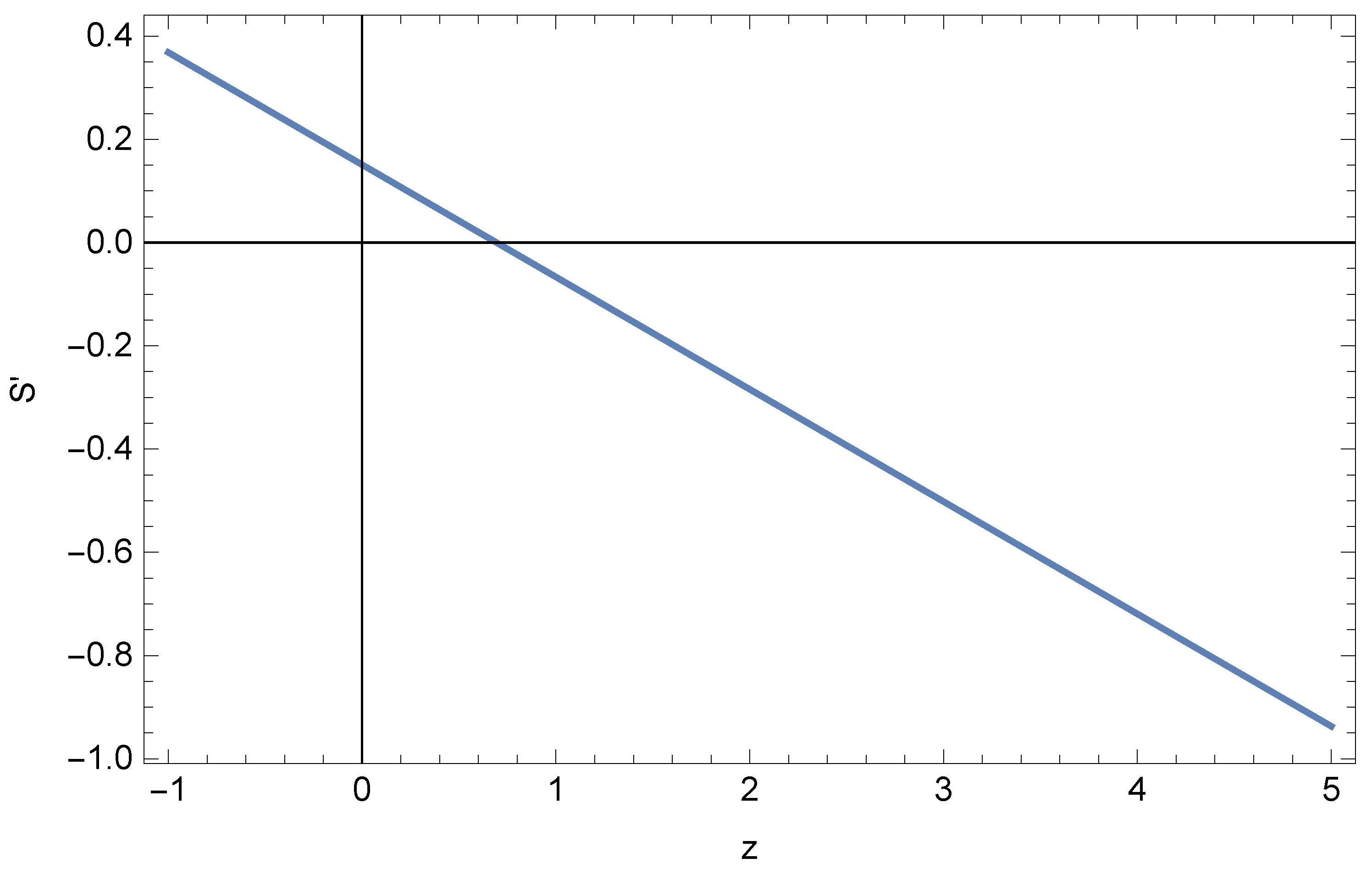
written in terms of the cosmographic set of parameters, i.e., $H_0,q_0,j_0$. Here, we considered second order expansions of all quantities involved in Equation (14). The entropy variation is negative after a given redshift, as one can notice from the analysis of the shape in Figure 1. At first order, its sign depends upon the first derivative of the total equation of state at $z=0$. The redshift at which the entropy variation vanishes is the transition redshift, where dark energy starts to dominate. Following the approximations: $\omega \sim -1+{\omega }_{1}z,\mathcal{V}\sim {\mathcal{V}}_0(1-3z)$ and looking at Figure 2, we notice that as a byproduct of dark energy, the entropy tends to decrease at all times. The entropy variation becomes zero at the dark energy and matter transition. At future times, the entropy tends to zero, leading to a negative $\frac{d\mathcal{S}}{dz}$. This is compatible with the concordance model, indicating a situation of larger entropy as the universe increases its size. Moreover, the entropy tends to a constant value at high redshift and at future time, i.e., $z\to -1$, goes to another constant value, different from the one at $z\to \infty$. An interesting fact is that during the whole universe evolution, the entropy is approximatively a constant.

2.2. The Cosmographic Representation of Specific Heats

The standard definition of a specific heat is [31]:

$$\mathsf{C}\equiv \frac{\partial \widehat{U}}{\partial T},$$

(17)

in which one considers a thermodynamic function, here $\widehat{U}$, which implies the typology of specific heat. In this work, we are particularly interested in computing the specific heats at constant pressure P and volume $\mathcal{V}$. We need these specific heats since we want to reproduce the Mayer relation for perfect gas. Thus, we have:

$$\begin{array}{cc}\hfill \widehat{U}& =h,\hfill \end{array}$$

(18)

$$\begin{array}{cc}\hfill \widehat{U}& =U,\hfill \end{array}$$

(19)

in which h and U are the enthalpy and energy, respectively, for specific heats at constant pressure and volume. We can therefore write [32]:

$$\begin{array}{c}\hfill {\mathsf{C}}_V=\frac{\partial U}{\partial T},{\mathsf{C}}_P=\frac{\partial h}{\partial T},\end{array}$$

(20)

whose functional forms are given by [15]

$$U=\rho \mathcal{V},h=\left(\rho +P\right)\mathcal{V},$$

(21)

in which we adopted basic demands of thermodynamics applied to the FRW universe. It follows that to fully determine the specific heats, one needs to know the volume and temperature evolutions. Below, we propose our technique to fix those quantities.

2.3. The Volume and Its Evolution in Terms of the Redshift

To understand how the volume evolves in terms of the redshift z from Equation (21), it is possible to follow the simplest assumption leading to a universe radius given by: $r_u\propto a$. This prescription implies a volume $\mathcal{V}={\mathcal{V}}_0{a}^3$, where ${\mathcal{V}}_0\sim \frac{1}{H_0}$. This leads to exactly the same result that we employed for our considerations over the entropy and its variation. Although, in general, it would be enough to limit ourselves to $\mathcal{V}\propto a^3$, a few words can be here spent to better understand how departures from this case can modify the expected outcomes on the specific heats.

In particular, more complicated volume expansions are also possible, We refer to them as $\mathcal{V}={\mathcal{V}}_{0}f(a^3)$, which in principle turn out to be a possible choice. If we limit our attention to the simplest case $\propto a^3$, both U and h are positive defined. This guarantees that the weak energy condition is not violated. However, in the literature other approaches suggest different points of views, motivated by physical requirements, different from assuming the above radius $r_u$. In particular, one can imagine to have $r_u\propto H^{-1}$ [33,34,35]. In general such a choice would reproduce a causal region different from the sphere $\propto a^3$, albeit at small redshift regime, i.e., $z\ll 1$, one can continue to approximate the volume with the simplest choice of $\mathcal{V}\propto a^3$. To check this, using $a=\frac{1}{1+z}$ and

$$\frac{dz}{dt}=-(1+z)H,$$

(22)

expanding the volume $\mathcal{V}\propto H^{-3}$, around $z\ll 1$, we obtain a volume correction of the form:

$$\begin{array}{cc}\hfill \mathcal{V}& \approx {\mathcal{V}}_0{a}^{3}f(z),\hfill \end{array}$$

(23a)

$$\begin{array}{cc}\hfill f(z)& ={\left[\frac{1}{1+(z-1)z(1+(z-1)z)(1+z+z^2)}\right]}^3,\hfill \end{array}$$

(23b)

in which we recall the definition $H=-\frac{d}{dt}ln(1+z)$.

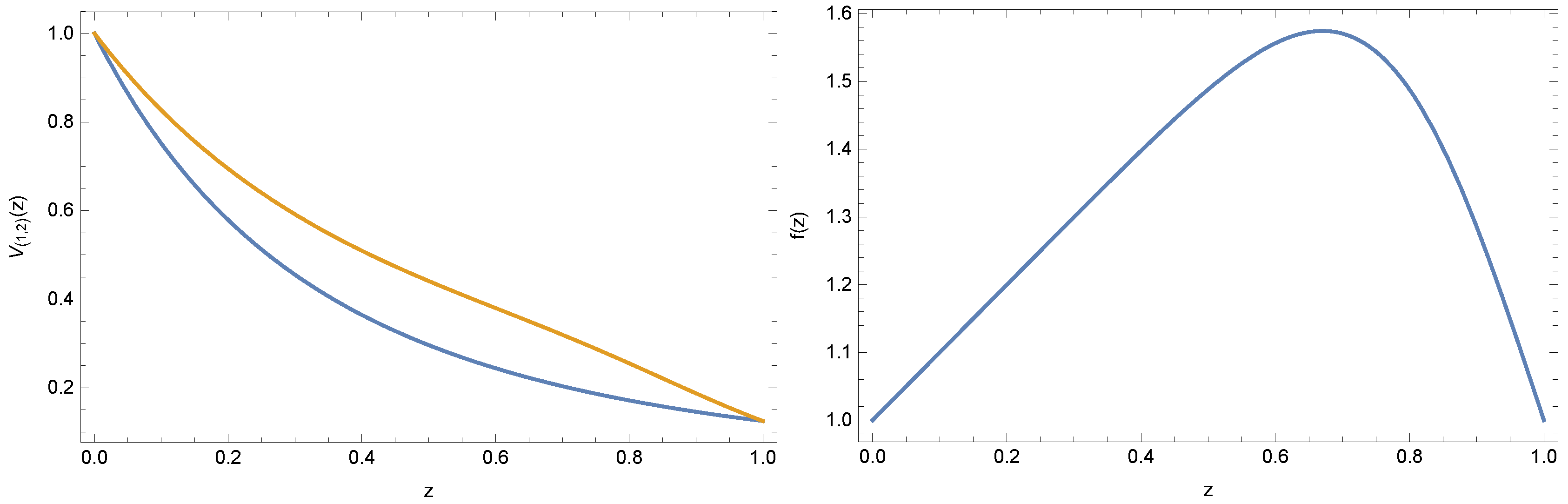
At small redshift, the function $f(z)$ represents a correction to the standard volume $\mathcal{V}\propto a^3$, which increases its importance in the whole volume magnitude as the redshift increases. The plot of $f(z)$, together with the volume variation are reported in Figure 3.

The net action of $f(z)$ on the volume is to increase its magnitude, but inside the sphere $z\le 1$ the increasing of $\mathcal{V}$ does not significantly influence the analysis. In other words, the two volumes become different outer this redshift limit, i.e., as $z\ge 1$. Since cosmography is built up at small redshift domains, it is licit to assume both the two approaches for fixing the universe volume and in particular to find out a trick able to reproduce the two quantities into a single scheme. Indeed, since, at the very small redshifts, the effects of $f(z)$ are to enlarge the volume $\propto a^{-3}$, we can assume a volume of the form (This is however a coarse-grained approach and more refined analyses are requested to check whether the influence of different volumes may change the thermodynamics in FRW.). $\mathcal{V}={\mathcal{V}}_0{(1+z)}^{-3}$, with a different value of ${\mathcal{V}}_0$. So that, $\mathsf{C}=\frac{d\tilde{U}}{dz}{\left(\frac{\partial T}{dz}\right)}^{-1}$, and using Equation (21) and the Friedman equations, we obtain

$${\mathsf{C}}_V=\frac{1}{T^{\prime }}\frac{dU}{dz}=\frac{3V_0{a}^3}{8\pi G{T}^{\prime }}\left(\frac{d{H}^2}{dz}-3a{H}^2\right),$$

(24)

and

$${\mathsf{C}}_P=\frac{1}{T^{\prime }}\frac{dh}{dz}=\frac{1}{T^{\prime }}\frac{dU}{dz}+\frac{V_0{a}^3}{T^{\prime }}\left(\frac{dP}{dz}-3aP\right),$$

(25)

where the prime denotes differentiation with respect to the redshift z. Once the volume and the specific heat definitions have been discussed, we need to understand how the temperature evolves in time. Unfortunately, without knowing the temperature evolution, it is not possible to understand how the Mayer relation works and also if it is valid for dark energy at different redshift regimes. To bypass this problem, we can recall that the universe’s temperature is fueled by all contributions coming from dark energy, matter, neutrinos and so forth. The analysis on how temperature evolves in terms of $a(t)$ is an open quest of modern cosmology. Indeed, the temperature reported in Equation (8) depends on the model under exam and turns out to be model-dependent. To overcome this issue, instead of using Equation (8), one can simply use an alternative parametrization, suitable inside the interval $z\le 1$. In other words, one needs a simpler approach to the temperature evolution in order to reconstruct the specific heats, without passing through the cosmological model definition.

The parametrization of our work would need that dark energy temperature is not dominant over the other contributions and since its magnitude has not been measured so far, we take a whole parametrization, following the standard recipe. We thus have [36]:

$$\frac{T}{T_0}=a^{-\delta },$$

(26)

which fulfills the requirements that we mentioned above. In principle, modifying the temperature definition with the parametrization (26) implies a different use of cosmic distances. This is intimately related to the duality problem [37,38] between the luminosity and angular distances. In this work, we assume that $\delta \sim 0$ and may be parameterized by $\delta =\beta -1$, with $\beta \simeq 1$.

3. The Evolution of Specific Heats

In this section, we conclude how the specific heats can be built up with the above requirements, discussed in the previous sections. In particular, assuming $T=T_0{(1+z)}^{\delta }$, by means of Equations (24) and (25), we obtain

$${\mathsf{C}}_V=\frac{\alpha }{2\delta }{H}^2\frac{2q-1}{{(1+z)}^{3+\delta }},$$

(27)

and

$${\mathsf{C}}_P=\frac{\alpha }{\delta }{H}^2\frac{j-1}{{(1+z)}^{3+\delta }},$$

(28)

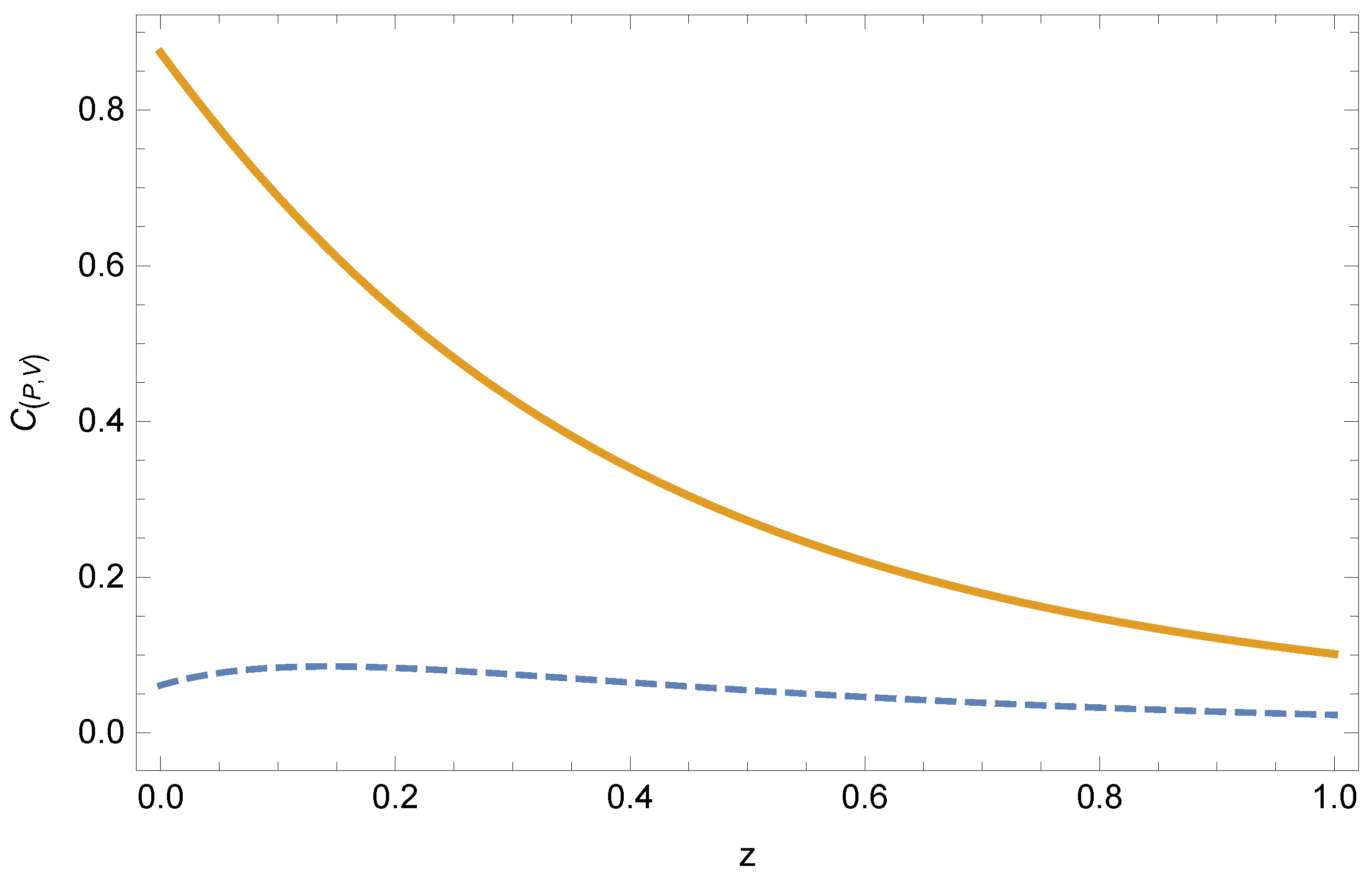
where $\alpha \equiv \frac{{\mathcal{V}}_0}{4\pi G{T}_0}$. To plot their evolutions, since $H^2$ is model dependent, we adopt the following strategy:

$$H_{(2)}=H_0+\frac{dH}{dz}z+\frac{d^{2}H}{d{z}^2}{z}^2=H_0\left[1+(1+q_0)z+\frac{1}{2}(j_0^2-q_0)z^2\right],$$

(29)

since H is rewritable in terms of $q_0$ which is model independent and can be measured alone (Here, there is a degeneracy between cosmographic coefficients, i.e., $H_0$, $q_0$ and $j_0$.). The plots are reported in Figure 4, with the following values for the cosmographic parameters [39]:

$$\begin{array}{cc}\hfill H_0& ={69.96}_{-1.16}^{+1.12},\hfill \end{array}$$

(30a)

$$\begin{array}{cc}\hfill q_0& =-{0.561}_{-0.042}^{+0.055},\hfill \end{array}$$

(30b)

$$\begin{array}{cc}\hfill j_0& ={0.999}_{-0.468}^{+0.346}.\hfill \end{array}$$

(30c)

Under this scheme, one can invoke the simplest framework to enable the cosmic speed up to emerge. In particular, one can assume dark energy as a perfect gas, i.e., the simplest approach within the energy momentum tensor of Einstein’s gravity. If a perfect gas works fairly well in describing the universe dynamics, there would be no reason a priori to assume a more complicated expression for dark energy, e.g., for example a liquid, a real gas, and so on.

It follows that if dark energy is a gas, the difference between the two specific heats is constant. This difference obeys the Mayer relation, valid for all perfect gas. This leads, as simplest case, to:

$${\mathsf{C}}_P-{\mathsf{C}}_V=\frac{\alpha }{2\delta }{H}_{(2)}^2\frac{2j-2q-1}{{(1+z)}^{3+\delta }},$$

(31)

and by virtue of:

$${\mathsf{C}}_P-{\mathsf{C}}_V=\mathcal{R}>0,$$

(32)

with $\mathcal{R}$ the gas constant, we guarantee that the Mayer relation holds. Hence, one has at least to assume that the difference between the two specific heats is positive. So, one has:

$$j-q>\frac{1}{2},$$

(33)

which is always valid, i.e., it is not circumscribed at our time only. Since j and q are in principle quantities which evolve in time, it is natural to expect regions in which the aforementioned relation does not hold. In those regions, the dark energy nature is not the one of a gas and relation (33) loses its validity. Since dark energy starts being dominant over matter at the transition time, it is useful to investigate what happens at the corresponding redshift. Indeed, at the transition between dark energy and matter, one gets $q_{tr}=0$, leading to:

$$j_{tr}>\frac{1}{2},$$

(34)

which represents a compatible relation for the jerk parameter, in terms of modern requirements of cosmography. Assuming the $\mathrm{\Lambda }$CDM model, for example, one has $j_{\mathrm{\Lambda }CDM}=1$ at all stages of universe evolution. This is compatible with Equation (34). The same equation permits one to circumscribe those dark energy models which do not satisfy either Equations (33) and (34). In other words, our approach represents an alternative method, based on thermodynamics, to discriminate dark energy models and to select those ones which better behave at late times.

4. Application to Observational Cosmology

In this section, we discuss some implications of our treatment in the context of observational cosmology. In particular, one of the most relevant trick to compare the theoretical framework above reported directly with data is to rewrite the luminosity distance in terms of $\mathcal{S}$ and $C_{h,V}$, using cosmography. The same procedure can be performed with other distances, such as angular, photon distance and so forth. Here, we limit to the luminosity distance $d_L$ only. Thus, we consider in function of z we can write down:

$$d_L=\frac{1}{a(t)}{\int }_t^{t_0}\frac{d{t}^{\prime }}{a(t^{\prime })}=(1+z){\int }_0^z\frac{d{z}^{\prime }}{H(z^{\prime })},$$

(35)

and at third order, we have:

$$\begin{array}{cc}\hfill d_L^{(3)}& \approx \frac{z}{H_0}\left(1+{\alpha }_{1}z+{\alpha }_2{z}^2+\dots \right),\hfill \end{array}$$

(36a)

$$\begin{array}{cc}\hfill {\alpha }_1& =\frac{1}{2}-\frac{q_0}{2},\hfill \end{array}$$

(36b)

$$\begin{array}{cc}\hfill {\alpha }_2& =\frac{q_0^2}{2}-\frac{1}{6}+\frac{q_0}{6}-\frac{j_0}{6}.\hfill \end{array}$$

(36c)

At the simplest level in which $\rho \mathcal{V}/T\equiv \mathrm{const}$, we have:

$$\begin{array}{cc}\hfill {\mathcal{S}}_0& =\frac{2}{3}(q_0+1),\hfill \\ \hfill \end{array}$$

(37a)

$$\begin{array}{cc}\hfill {\mathcal{S}}_0^{\prime }& =\frac{2}{3}\left[-3+j_0+3{\mathrm{\Omega }}_m(1+q_0)+\delta +q_0(-4-2q_0+\delta )\right],\hfill \\ \hfill \end{array}$$

(37b)

$$\begin{array}{cc}\hfill {\mathsf{C}}_{V,0}& =\frac{\alpha }{2\delta }{H}_0^2(2q_0-1),\hfill \\ \hfill \end{array}$$

(37c)

$$\begin{array}{cc}\hfill {\mathsf{C}}_{P,0}& =\frac{\alpha }{\delta }{H}_0^2(j_0-1),\hfill \end{array}$$

(37d)

we have:

$$\begin{array}{cc}\hfill d_L\left({\mathcal{S}}_0,{\mathcal{S}}_0^{\prime }\right)& =d_H(z)\left[1-\frac{3}{2}{\mathcal{S}}_0+\frac{1}{8}(-2{\mathcal{S}}_0^{\prime }+{\mathcal{S}}_0(-10+6{\mathrm{\Omega }}_m+3{\mathcal{S}}_0+2\delta )\right],\hfill \\ \hfill \end{array}$$

(38a)

$$\begin{array}{cc}\hfill d_L\left({\mathsf{C}}_{P,0},{\mathsf{C}}_{V,0}\right)& =d_H(z)\left[1-\frac{1}{4}\left(1-\frac{2{\mathsf{C}}_{V,0}}{H_0^2}\right)z+\frac{1}{24}\left(-3+\frac{12{\mathsf{C}}_{V,0}}{H_0^4}-\frac{4{\mathsf{C}}_{P,0}}{H_0^2}+\frac{16{\mathsf{C}}_{V,0}}{H_0^2}\right)z^2\right],\hfill \end{array}$$

(38b)

where $d_H(z)\equiv \frac{z}{H_0}$. Making use of Equation (30), we thus obtain:

$$\begin{array}{cc}\hfill \mathcal{S}& ={0.293}_{-0.028}^{+0.037},\hfill \\ \hfill \end{array}$$

(39a)

$$\begin{array}{cc}\hfill \frac{d\mathcal{S}}{dz}& <0,\hfill \end{array}$$

(39b)

and

$$\begin{array}{cc}\hfill {\mathsf{C}}_P& =-{0.001}_{-0.229}^{+0.169},\hfill \\ \hfill \end{array}$$

(40a)

$$\begin{array}{cc}\hfill {\mathsf{C}}_V& =-{1.061}_{-0.038}^{+0.044}.\hfill \end{array}$$

(40b)

Those limits and constraints are compatible with the concordance model, albeit small departures seem to be present. In general, together with Equations (33) and (34), one can discriminate among dark energy models, the ones which better reproduce the aforementioned bounds.

However, in [29] constraints imposed by different data surveys are apparently in conflict with generic versions of dark energy fluids, where time-dependent barotropic factors are supposed. Indeed, constraints imposed by thermodynamics may indicate that dark energy fluids may be unphysical. To figure this out, we need future and refined numerical outcomes from cosmic data sets which will provide evidences against a time variation of $\omega$. In principle, using the results presented in this paper, one can match cosmic distances with data in order to verify the goodness of whatever dark energy models. Again, the results presented in [29] do not seem to contradict the perspective of present work.

In the $\mathrm{\Lambda }$CDM case, the expected outcomes are inside the above intervals, however the dark fluid approach [40,41] is also able to reproduce analogous results. In [32], it has been established that similar results are much more compatible with a one-fluid approach in which dark energy emerges as due to dark matter and baryons, by simply imposing $c_s=0$. Summing up: if a gaseous component enters Einstein’s equations, without invoking dark energy, it is possible to require it by invoking the validity of Equation (31). The corresponding one fluid has the advantage to allow dark energy to emerge and is defined by:

$$\begin{array}{cc}\hfill \frac{H^2}{H_0^2}& =\frac{{\rho }_{d0}}{1+K}\left(1+\frac{K}{a^3}\right),\hfill \end{array}$$

(41a)

$$\begin{array}{cc}\hfill c_s& =0,\hfill \end{array}$$

(41b)

$$\begin{array}{cc}\hfill {\omega }_{DE}& =\omega ,\hfill \end{array}$$

(41c)

where $K=-P_0^{-1}({\rho }_{d0}+P_0)$ and ${\omega }_{DE}$ is the unique equation of state.

In other words, without assuming any cosmological constant a priori, it is possible to get the cosmic speed up with a constant term pushing up the universe to accelerate, different from the cosmological constant with the advantage to be modeled as a perfect gas. The main difference between the concordance model and the dark fluid framework lies on the form of $\omega$ which is exactly the same as ${\omega }_{DE}$. Hence, the model is simpler than the concordance paradigm made by two fluids, i.e., matter and $\mathrm{\Lambda }$. Our model, moreover, comes from assuming a simple gas (throughout the manuscript, we did not give relevance to the typology of gas involved into our scheme. However, future discussions on its form are essential to understand the dark fluid origin. This will be object of future developments.) inside the thermodynamic definitions of specific heats. In general, one cannot conclude that this model is better than the concordance paradigm. There is, in fact, no reasons to assume a vanishing cosmological constant at early times, hence, how is it possible to describe the cosmic speed up mimicking the cosmological constant with a thermodynamic dark fluid, but assuming negligible the $\mathrm{\Lambda }$’s contribution?

In addition, since the dark fluid model well passes high-redshift tests [42], it is plausible to reconsider it to describe the whole dynamics. As mentioned above, this prerogative will be possible if one shows how to remove the quantum vacuum energy fluctuations from Einstein’s energy momentum tensor, or if one can take $\mathrm{\Lambda }$ negligibly small if compared to the dark fluid magnitude (due to the fine-tuning issue, the $\mathrm{\Lambda }$’s magnitude is enormous than the one measured by cosmological observations.). This treatment is essential to discriminate between the two models, since a strong degeneracy occurs between the concordance paradigm and the dark fluid [43].

Another interesting possibility of our treatment is to take into account the role played by singularities, discriminating the typologies of singularities one expects at future and past times through the use of thermodynamics. In other words, for example, given a dark energy model, it would be possible to replace the classifications made by [44] shifting from the use of the equation of state to entropy and specific heats. This would represent a new technique toward the singularity classification directly making use of the dark energy thermodynamics.

5. Conclusions

We revised some aspects of dark energy’s thermodynamics, investigating how entropy, its variation and specific heats can be used to discriminate dark energy models. Assuming a flat universe, embedded in a FRW metric, we considered adiabatic heat exchanges and we wrote the entropy and specific heats through cosmographic model-independent quantities. Thus, we traced evolutions in terms of z and we characterized the regions in which cosmographic limits are compatible with observations. To do so, we also assumed dark energy as a perfect gas, in the simplest approach in which the Mayer relation is preserved. We found limits over the entropy and its variation compatible with the standard model. Moreover, we found that the Mayer relation holds if $j-q>\frac{1}{2}$. The former result turns out to be general such that, even at the transition time, the jerk parameter j cannot violate the condition: $j_{tr}>\frac{1}{2}$. This outcome rules out those models which predict opposite cases, whereas turns out to be compatible with the concordance paradigm. We discussed how to reconstruct dark energy’s entropy from specific heats and we finally compute both entropy and specific heats into the luminosity distance $d_L$. Keeping in mind the numerical bounds of cosmography, we gave constraints over the entropy and specific heats. We thus compare our bounds with the $\mathrm{\Lambda }$CDM model, highlighting that a constant dark energy term seems to be only slightly compatible with the so-obtained specific heat thermodynamics. Assuming, indeed, a zero sound speed, one can recover a dark fluid counterpart, which extends the concordance model without postulating any cosmological constant at the beginning. Future developments can be useful to discriminate whether the dark fluid is effectively responsible for the cosmic speed up. Since there exists a degeneracy between it and the concordance paradigm, one needs to demonstrate that $\mathrm{\Lambda }$ is smaller than the dark fluid magnitude. Further, other interesting treatments will develop on the possibility to produce cosmological models from the above requirements and to investigate how departures from Mayer’s relation can be used to characterize dark energy at redshifts $z>1$. Finally, it would be even possible to re-obtain the singularity classifications at future and past times, commonly made by using the equation of state, through an analogous view made by thermodynamical quantities, such as $\mathcal{S}$, ${\mathsf{C}}_P$ and ${\mathsf{C}}_V$.

References

- Planck 2013 Results. XVI. Cosmological Parameters. Available online: https://www.aanda.org/articles/aa/abs/2014/11/aa21591-13/aa21591-13.html (accessed on 11 October 2017).
- Copeland, J.E.; Sami, M.; Tsujikawa, S. Dynamics of Dark Energy. Int. J. Mod. Phys. D 2006, 15, 1753–1936. [Google Scholar] [CrossRef]
- Bamba, K.; Capozziello, S.; Nojiri, S.; Odintsov, S.D. Dark energy cosmology: The equivalent description via different theoretical models and cosmography tests. Astroph. Sp. Sci. 2012, 342, 155. [Google Scholar] [CrossRef]
- Nojiri, S.; Odintsov, S.D. Unified cosmic history in modified gravity: From F(R) theory to Lorentz non-invariant models. Phys. Rep. 2011, 505, 59. [Google Scholar] [CrossRef]
- Nojiri, S.; Odintsov, S.D.; Oikonomou, V.K. Modified Gravity Theories on a Nutshell: Inflation, Bounce and Late-time Evolution. Phys. Rep. 2017, 692, 1. [Google Scholar] [CrossRef]
- Riess, A.G.; Filippenko, A.V.; Challis, P.; Clocchiatti, A.; Diercks, A.; Garnavich, P.M.; Gilliland, R.L.; Hogan, C.J.; Jha, S.; Kirshner, R.P.; et al. Observational Evidence from Supernovae for an Accelerating Universe and a Cosmological Constant. Astron. J. 1998, 116, 1009. [Google Scholar] [CrossRef]
- Perlmutter, S.; Aldering, G.; Goldhaber, G.; Knop, R.A.; Nugent, P.; Castro, P.G.; Deustua, S.; Fabbro, S.; Goobar, A.; Groom, D.E.; et al. Measurements of Omega and Lambda from 42 High-Redshift Supernovae. Astrophys. J. 1999, 517, 565. [Google Scholar] [CrossRef]
- Weinberg, S. The cosmological constant problem. Rev. Mod. Phys. 1989, 61, 1. [Google Scholar] [CrossRef]
- Li, M.; Li, X.D.; Wang, S.; Wang, Y. Dark Energy. Com. Theor. Phys. 2011, 56, 525–604. [Google Scholar] [CrossRef]
- Lima, J.A.S.; Alcaniz, J.S. Thermodynamics, Spectral Distribution and the Nature of Dark Energy. Phys. Lett. B 2004, 600, 191. [Google Scholar] [CrossRef]
- Misner, C.W.; Thorne, K.S.; Wheeler, J.A. Gravitation; W. H. Freeman: New York, NY, USA, 1973. [Google Scholar]
- Krasinski, A.; Quevedo, H.; Sussman, R. On the thermodynamical interpretation of perfect fluid solutions of the Einstein equations with no symmetry. J. Math. Phys. 1997, 38, 2602. [Google Scholar] [CrossRef]
- Lynden-Bell, D.; Wood, R. The gravo-thermal catastrophe in isothermal spheres and the onset of red-giant structure for stellar systems. Mon. Not. R. Astr. Soc. 1968, 138, 495. [Google Scholar] [CrossRef]
- Lynden-Bell, D. Negative specific heat in astronomy, physics and chemistry. Phys. A Stat. Mech. Appl. 1999, 263, 1–4. [Google Scholar] [CrossRef]
- Padmanabhan, T. Statistical mechanics of gravitating systems. Phys. Rep. 1990, 188, 285. [Google Scholar] [CrossRef]
- Einarsson, B. Conditions for negative specific heat in systems of attracting classical particles. Phys. Lett. A 2004, 332, 335–344. [Google Scholar] [CrossRef]
- Harrison, E. Observational tests in cosmology. Nature 1976, 260, 591. [Google Scholar] [CrossRef]
- Visser, M. General relativistic energy conditions: The Hubble expansion in the epoch of galaxy formation. Phys. Rev. D 1997, 56, 7578. [Google Scholar] [CrossRef] [Green Version]
- Dunsby, P.K.S.; Luongo, O. On the theory and applications of modern cosmography. Int. J. Geom. Meth. Mod. Phys. 2016, 13, 1630002. [Google Scholar] [CrossRef]
- Aviles, A.; Gruber, C.; Luongo, O.; Quevedo, H. Cosmography and constraints on the equation of state of the Universe in various parametrizations. Phys. Rev. D 2012, 86, 123516. [Google Scholar] [CrossRef]
- Luongo, O. Dark energy from a positive jerk parameter. Mod. Phys. Lett. A 2013, 28, 1350080. [Google Scholar] [CrossRef]
- Visser, M. Jerk, snap and the cosmological equation of state. Class. Quant. Grav. 2004, 21, 2603. [Google Scholar] [CrossRef]
- Cattoen, C.; Visser, M. Cosmographic Hubble fits to the supernova data. Phys. Rev. D 2008, 78, 063501. [Google Scholar] [CrossRef]
- Busti, V.C.; Dunsby, P.K.S.; de la Cruz-Dombriz, A.; Saez-Gomez, D. Is cosmography a useful tool for testing cosmology? Phys. Rev. D 2015, 92, 123512. [Google Scholar] [CrossRef]
- Weinberg, S. Entropy generation and the survival of protogalaxies in an expanding universe. Astrop. J. 1971, 168, 175. [Google Scholar] [CrossRef]
- Lima, J.A.S.; Germano, A.S.M. On the equivalence of bulk viscosity and matter creation. Phys. Lett. A 1992, 170, 373. [Google Scholar] [CrossRef]
- Silva, R.; Lima, J.A.S.; Calvão, M.O. Temperature evolution law of imperfect relativistic fluids. Gen. Rel. Grav. 2002, 34, 865. [Google Scholar] [CrossRef]
- Silva, R.; Goncalves, R.S.; Alcaniz, J.S.; Silva, H.H.B. Thermodynamics and dark energy. Astron. Astroph. 2012, 537, A11. [Google Scholar] [CrossRef]
- Barboza, E.M., Jr.; Nunes, R.C.; Abreu, E.M.C.; Neto, J.A. Thermodynamic aspects of dark energy fluids. Phys. Rev. D 2015, 92, 083526. [Google Scholar] [CrossRef]
- Schutz, B.F., Jr. Perfect fluids in general relativity: Velocity potentials and a variational principle. Phys. Rev. D 1970, 2, 12. [Google Scholar] [CrossRef]
- Kundu, P.K.; Cohen, I.M. Fluid Mechanics; Academic Press: San Diego, CA, USA, 2004. [Google Scholar]
- Luongo, O.; Quevedo, H. Cosmographic study of the universe’s specific heat: A landscape for cosmology? Gen. Rel. Grav. 2014, 46, 1649. [Google Scholar] [CrossRef]
- Cai, R.G.; Kim, S.P. First law of thermodynamics and Friedmann equations of Friedmann-Robertson-Walker universe. J. High Energy Phys. 2005. [Google Scholar] [CrossRef]
- Cai, R.G.; Cao, L.M.; Hu, Y.P. Hawking radiation of an apparent horizon in a FRW universe. Class. Quant. Grav. 2009, 26, 155018. [Google Scholar] [CrossRef]
- Del Campo, S.; Duran, I.; Herrera, R.; Pavon, D. Three thermodynamically based parametrizations of the deceleration parameter. Phys. Rev. D 2012, 86, 083509. [Google Scholar] [CrossRef]
- Lima, J.A.S.; Silva, A.I.; Viegas, S.M. Is the radiation temperature-redshift relation of the standard cosmology in accordance with the data? Mont. Not. R. Astr. Soc. 2000, 312, 747. [Google Scholar] [CrossRef]
- Avgoustidis, A.; Verde, L.; Jimenez, R. Consistency among distance measurements: Transparency, BAO scale and accelerated expansion. J. Cosmol. Astropart. Phys. 2009. [Google Scholar] [CrossRef]
- Yang, X.; Yu, H.R.; Zhang, Z.S.; Zhang, T.J. An improved method to test the distance-duality relation. Astroph. J. Lett. 2013, 777, L24. [Google Scholar] [CrossRef]
- Gruber, C.; Luongo, O. Cosmographic analysis of the equation of state of the universe through Padé approximations. Phys. Rev. D 2014, 89, 103506. [Google Scholar] [CrossRef]
- Luongo, O.; Quevedo, H. A unified dark energy model from a vanishing speed of sound with emergent cosmological constant. Int. J. Mod. Phys. D 2014, 23, 1450012. [Google Scholar] [CrossRef]
- Luongo, O.; Quevedo, H. An Expanding Universe with Constant Pressure and no Cosmological Constant. Astroph. Sp. Sci. 2012, 338, 345. [Google Scholar] [CrossRef]
- Aviles, A.; Cervantes-Cota, J.L. Dark degeneracy and interacting cosmic components. Phys. Rev. D 2011, 84, 083515. [Google Scholar] [CrossRef]
- Dunsby, P.K.S.; Luongo, O.; Reverberi, L. Dark energy and dark matter from an additional adiabatic fluid. Phys. Rev. D 2016, 94, 083525. [Google Scholar] [CrossRef]
- Nojiri, S.; Odintsov, S.D.; Tsujikawa, S. Properties of singularities in the (phantom) dark energy universe. Phys. Rev. D 2005, 71, 063004. [Google Scholar] [CrossRef]
Figure 1.
Plot of the entropy function in terms of the redshift z, with indicative values , , , , and . The temperature is the usual cosmic background temperature, i.e., . The plot is performed up to , to be compatible with the approximation made on at our time. The entropy tends to vanish at future time. It provides a pick close to , whereas it tends to decrease as the redshift increases. Its values are essentially small at all times of universe’s evolution. In the fiducial model the entropy is exactly zero, i.e., . Any departures from the concordance paradigm would lead to small departures on magnitude.
Figure 2.
Plot of the entropy variation in terms of the redshift. The axis label refers to . Again, we used the following indicative values , , , , and . The change of slope is expected at future time.
Figure 3.
Plots of both the volumes (left figure), i.e., and respectively, in the redshift domain in which no significant departures from the simplest case are expected. Plot of the function (right figure) in terms of the redshift in the same domain as above.
Figure 4.
Plots of both the specific heats using Equation (30), with arbitrary fixed , inside the redshift domain . The dashed line refers to the specific heat at constant volume, whereas the thick line to the specific heat at constant pressure.
© 2017 by the author. Licensee MDPI, Basel, Switzerland. This article is an open access article distributed under the terms and conditions of the Creative Commons Attribution (CC BY) license (http://creativecommons.org/licenses/by/4.0/).
Share and Cite
MDPI and ACS Style
Luongo, O. Cosmographic Thermodynamics of Dark Energy. Entropy 2017, 19, 551. https://doi.org/10.3390/e19100551
AMA Style
Luongo O. Cosmographic Thermodynamics of Dark Energy. Entropy. 2017; 19(10):551. https://doi.org/10.3390/e19100551
Chicago/Turabian StyleLuongo, Orlando. 2017. "Cosmographic Thermodynamics of Dark Energy" Entropy 19, no. 10: 551. https://doi.org/10.3390/e19100551
Note that from the first issue of 2016, this journal uses article numbers instead of page numbers. See further details here.